| Issue |
A&A
Volume 686, June 2024
|
|
|---|---|---|
| Article Number | A51 | |
| Number of page(s) | 10 | |
| Section | Stellar atmospheres | |
| DOI | https://doi.org/10.1051/0004-6361/202347924 | |
| Published online | 28 May 2024 | |
Energetic particle activity in AD Leo: Detection of a solar-like type-IV burst
1
Rosseland Centre for Solar Physics, University of Oslo,
Postboks 1029 Blindern,
N-0315
Oslo,
Norway
e-mail: atul.mohan@nasa.gov
2
Institute of Theoretical Astrophysics, University of Oslo,
Postboks 1029 Blindern,
N-0315
Oslo,
Norway
3
The Catholic University of America,
620 Michigan Avenue, N.E.
Washington,
DC
20064,
USA
4
NASA Goddard Space Flight Center,
8800 Greenbelt Road,
Greenbelt,
MD
20771,
USA
5
Center for Solar-Terrestrial Research, New Jersey Institute of Technology,
323 M L King Jr Boulevard,
Newark,
NJ
07102-1982,
USA
Received:
9
September
2023
Accepted:
29
January
2024
Context. AD Leo is a young and active M dwarf with high flaring rates across the X-ray-to-radio bands. Flares accelerate particles in the outer coronal layers and often impact exo-space weather. Wide-band radio dynamic spectra let us explore the evolution of particle acceleration activity across the corona. Identifying the emission features and modelling the mechanisms can provide insights into the possible physical scenarios driving the particle acceleration processes.
Aims. We performed an 8 h monitoring of AD Leo across the 550-850 MHz band using upgraded-Giant Metrewave Radio Telescope (uGMRT). The possible flare and post-flare emission mechanisms are explored based on the evolution of flux density and polarisation.
Methods. The python-based module, Visibility Averaged Dynamic spectrum (VISAD), was developed to obtain the visibility-averaged wide-band dynamic spectra. Direct imaging was also performed with different frequency-time averaging. Based on existing observational results on AD Leo and on solar active region models, radial profiles of electron density and magnetic fields were derived. Applying these models, we explored the possible emission mechanisms and magnetic field profile of the flaring active region.
Results. The star displayed a high brightness temperature (TB≈ 1010−1011 K) throughout the observation. The emission was also nearly 100% left circularly polarised during bursts. The post-flare phase was characterised by a highly polarised (60–80%) solar-like type IV burst confined above 700 MHz.
Conclusions. The flare emission favours a Z-mode or a higher harmonic X-mode electron cyclotron maser emission mechanism. The >700 MHz post-flare activity is consistent with a type-IV radio burst from flare-accelerated particles trapped in magnetic loops, which could be a coronal mass ejection (CME) signature. This is the first solar-like type-IV burst reported on a young active M dwarf belonging to a different age-related activity population (‘C’ branch) compared to the Sun (‘I’ branch). We also find that a multipole expansion model of the active region magnetic field better accounts for the observed radio emission than a solar-like active region profile.
Key words: stars: activity / stars: coronae / stars: flare / stars: low-mass / stars: magnetic field / radio continuum: stars
© The Authors 2024
 Open Access article, published by EDP Sciences, under the terms of the Creative Commons Attribution License (https://creativecommons.org/licenses/by/4.0), which permits unrestricted use, distribution, and reproduction in any medium, provided the original work is properly cited.
This article is published in open access under the Subscribe to Open model. Subscribe to A&A to support open access publication.
1 Introduction
Low-mass main-sequence stars of spectral type M (M dwarfs) make up the most numerous stellar type in our galaxy. They also have the highest occurrence rate of Earth-like exoplanets in their habitable zones (Bashi et al. 2020). Meanwhile, M-dwarfs form the most active population among cool main-sequence stars with relatively high values of flaring rates, X-ray-to-bolometric flux ratio, and other activity metrics (see Donati & Landstreet 2009 for a review). Moreover, the younger stars are more active with stronger magnetic fields and faster rotation rates (e.g. Vidotto et al. 2014; Lund et al. 2020). Stellar flares cause energetic space-weather events including the release of energetic particles, intense high-energy radiation and large-scale eruptions, which threaten the stability of planetary atmospheres and hence the habitability. So, it is important to understand the mechanism, evolution, and space-weather consequences of M dwarf flares.
For this study, we chose the very active M3.5V star AD Leo located at ≈5 pc from the Sun. The star is proposed to host a planet (Tuomi et al. 2018), though the detection was later refuted (Carleo et al. 2020). The star has a typical mean optical flaring rate of ≈0.6 h−1 (Dal 2020). AD Leo displays high levels of chromospheric and coronal activity in several spectral lines and X-ray bands (Crespo-Chacón et al. 2006). Villadsen & Hallinan (2019) estimated a radio flaring rate of ≈0.2−0.3 h−1 with a coherent burst emission duty cycle of ≈20–25% in the 0.34–1.4 GHz range.
Flare emission in the metrewave band is sensitive to various coherent emission signatures from flare-accelerated electrons either trapped in low-coronal magnetic field structures or streaming across coronal layers (e.g. Wild 1970; McLean & Labrum 1985; Bastian 1990; Melrose 2009, 2017; Zic et al. 2020; Vedantham 2021). The two prominent coherent emission mechanisms discussed in the literature include the electron cyclotron maser emission (ECME) and the plasma emission (Dulk 1985; Güdel 2002; Melrose 2017). ECME dominates when the ratio of plasma frequency to gyro-frequency (νp/νB) at the flare source region is less than 1.5 (Melrose & Dulk 1982; Melrose et al. 1984; Dulk 1985; Dulk & Winglee 1987). When νp/νB>3, the favoured emission mechanism is plasma emission (e.g. Ginzburg & Zhelezniakov 1958; Tsytovich & Kaplan 1969; Melrose & Sy 1972; Cairns & Melrose 1985; Melrose 2009). Depending on the emission mechanism, the coherent emission frequencies correspond to either the fundamental mode or the harmonics of the local plasma frequency (νp) or gyro-frequency (vB), letting us infer either the local density or magnetic field strength, respectively. Apart from the flare emission, M dwarfs are also known to display non-flaring (or non-impulsive) continuum emission with a high brightness temperature (TB) (e.g. White et al. 1989; Bastian 1990). In a few GHz (<2 GHz) bands, the continuum TB ranges from ≈107−109 K (Osten & Bastian 2008; Villadsen & Hallinan 2019). In metrewavebands, TB can be even higher (e.g. Bastian 1994; Güdel 2002; Villadsen & Hallinan 2019). The continuum emission can form either from a gyrosynchrotron mechanism, or a combination of various coherent emission processes operating at multiple active regions (Bastian 1996; Benz 1996; Zaitsev et al. 1997).
There have been many studies that explored radio emission from AD Leo, reporting several flaring events. While instrumental limitations forced earlier studies to use only a few discontinuous narrow frequency bands (e.g. Spangler et al. 1974; Bastian et al. 1990), recent observations with continuous wide-band instruments have enabled spectroscopic explorations revealing rich variability in the dynamic spectrum (e.g. Osten & Bastian 2008; Villadsen & Hallinan 2019; Zhang et al. 2023). These studies have revealed several features such as fast pulsations at scales of ≈ms–min and high drift rates in the dynamic spectrum, often related to the propagation of energetic particles or spatiotemporal evolution of plasma instabilities in the associated active regions (e.g. Bastian et al. 1990; Osten & Bastian 2006, 2008; Zhang et al. 2023). However, much of these observations had been close to or above 1 GHz. Here, we present an 8 h monitoring of AD Leo across a wide sub-Giga Hertz band, which is expected to probe higher atmospheric layers than those probed by Giga Hertz bands. Though the original study was planned with simultaneous observation spanning from the X-ray to the radio band, only the radio observations were successful due to various technical issues. We present the results from metrewave observations here.
Section 2 provides the data and analysis methodology. Section 3.1 presents the different activity periods observed and the emission characteristics. Section 4 provides our inferences, and Sect. 5 summarises the conclusions.
2 Data and methodology
AD Leo was observed with uGMRT (Gupta et al. 2017) in Band 4 (550–850 MHz) from 3 December 2021, 21:17:41 UT to 4 December 2021, 04:17:41 UT at ≈5 s and ≈ 100 kHz time and frequency resolutions, respectively. The data were gathered in RR and LL polarisations, letting us explore the spectro-temporal evolution of the circular polarisation along with brightness temperature (TB) or flux density. The data analysis was done using the functionalities in the interferometric analysis package, Common Astronomy Software Applications (CASA; CASA Team 2022). The data were first flagged and calibrated using standard procedures. The flux calibrator was 3C 147, and the phase calibrator was 1021+219. Portions of data affected by radio frequency interference from terrestrial sources and systematic instrumental effects were identified and flagged manually. The automatic flagging routine in CASA, namely tfcrop, was also used. This was followed by bandpass calibration using the flux calibrator, and then by time-dependent gain calibration using the phase calibrator. The bandpass solution and the time-dependent gain solution were then extrapolated to the target star field. The calibrated target field data were further flagged using the Rflag routine in CASA. Initial imaging was done using the CASA task tclean in mtmfs mode, with nterms set to two and averaging over the entire observing time. This produced a mean model image for the entire spectral band, which was taken as the initial model, and self-calibration was performed in an iterative manner (Cornwell & Fomalont 1999) to improve it. After the second iteration, an optimal model was obtained. So, we stopped at the second iteration and adopted the CLEAN model of the iteration as the mean model image of the field of view for the observation period. The AD Leo emission at the phase centre was masked from the final model image, and the model visibilities were subtracted from the corrected data. The remaining corrected visibilities pertain to purely stellar emission. This stellar data were subjected to two forms of analysis as described below.
First, we developed a python-based package, Visibility Averaged Dynamic spectrum (VISAD), to extract the visibilities from a calibrated CASA measurement set (MS) and generate a dynamic spectrum (DS) with required time and frequency averaging. The package has routines to perform additional data flagging on the calibrated MS if required. The package uses CASA tasks inside a python environment and employs the parallel processing tools in python (multiprocessing1) enabling an analysis of several hours of wide-bandwidth datasets within a couple of minutes depending on the available machine cores. The module is made publicly available via GitHub2. We obtained both dynamic spectra and band-averaged light curves in Stokes I and V using VISAD. The Stokes V data were corrected as per the suggestions in Das et al. (2020) to adhere to the standard IAU/IEEE convention.
We also produced image spectral cubes for the entire observing period with varying time and frequency averaging, which were carefully chosen to detect the star with a signal-to-noise ratio (S/N) of at least five in every spectro-temporal slice. This exercise generated two data sets: a library of stellar spectra for different time bins spanning the entire observation period and a band-averaged stellar light curve. The spectra were generated with a resolution of 20 MHz and a time averaging of ≈2–3 min during the very active periods. During periods of weak activity, a 50 MHz averaging with 5–15 min time averaging was employed. We used the image cube information to cross-verify the flux densities obtained from a visibility-averaged DS for the flare period. The values matched within ≈ 15–20%. A source of this discrepancy is the additional flagging done in a couple of higher frequency channels while using VISAD. The presence of artefacts away from the source would also play a role in the observed difference in the flux density. In this work, we discuss the spectro-temporal nature of the observed activity, the possible physical mechanism, and infer physical properties of the emission region in the corona.
3 Results
3.1 Results from VISAD
Figure 1a shows the Stokes V dynamic spectrum from VISAD made with 100 s and 10 MHz averaging in the top panel. The bottom panels shows the band-averaged light curve obtained from VISAD in Stokes I and V, with 100 s averaging. Until 23:09:00 UT, we find multiple epochs of strong intermittent flaring activity, during which the stellar TB suddenly rises beyond 1011 K with circular polarisation levels between 60 and 90%. We note that the TB values reported are averaged over the entire stellar disc, thus the true TB will be higher depending on how small the area of the active region is compared to the size of the star. The flare rise phases are sudden and are followed by decay phases in both TB and polarisation fraction, as clearly seen in the band-averaged light curves. We mark this initial 2 h period as a period of strong activity. Analysing the typical flux levels to which Stokes V emission falls back after the sudden impulsive rise in the light curve, a basal Stokes V flux level is fixed at −2 mJy, corresponding to TB = −0.5 × 10¹¹ K. A similar exercise on the Stokes I light curve leads to a basal flux level of ≈4mJy (TB = 1.0 × 10¹¹ K), which is about twice the typical quiescent flux seen during the quasi-steady period, as noted in Fig. 1. The basal flux levels are used to define flaring epochs during the strong activity period. A flaring epoch is said to begin when the stellar flux rises above the basal flux level and ends when the flux falls back below the basal level. Based on this definition, four flaring epochs (F1–4; see Figs. 1b,c) with flare decay timescales of ≈5–30 min are identified in both of the Stokes light curves.
After the strong activity period, the star goes through ≈ 1.4 h period of weak activity between 2021-12-03 23:09:00 UT and 2021-12-04 00:24:00 UT (see Figs. 1b,c). This period is characterised by high Stokes V TB≈0.5−1.5×10¹¹, primarily the in higher frequency bands (≳700 MHz) as seen in the VISAD spectrum (Fig. 1a). The observed Stokes V and Stokes I TB is much brighter than the expected coronal temperature of ≈3 MK based on X-ray studies (e.g. van den Besselaar et al. 2003; Namekata et al. 2020). Additionally, the band-averaged flux light curves in both Stokes I and V demonstrate high polarisation levels of ≈50–90% during the weak activity period, with a gradually varying profile resultant from the dynamic spectral structure of the emission. Such emission characteristics after flares have been observed in the Sun as well and are interpreted as signatures of high-energy particles trapped in post-flare loops (Gergely 1986; Gopalswamy 2011; Hillaris et al. 2016; Morosan et al. 2019; Salas-Matamoros & Klein 2020). We believe that the same phenomenon is also behind the observed emission characteristics in this case.
After the weak activity period, we find that the Stokes V and I light curves tend to fluctuate around characteristic mean flux values of ≈−0.5 and 1.5 mJy with relatively low circular polarisation levels. We define this phase as the quasi-steady phase.
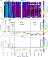 |
Fig. 1 Results from VISAD pipeline. (a) Stokes V dynamic spectrum. (b, c) Band-averaged light curves in Stokes V and I. The ordinate shows TB (left) and flux density (right), respectively. Different periods of activity are marked. Basal flux density levels in Stokes I and V are represented by dotted lines in the respective panels. We note that the TB values are nominal and simply highlight that the emission is via a coherent emission mechanism. Since the true source sizes are unknown, an average (i.e. across the whole unresolved stellar disc) TB is computed here. |
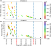 |
Fig. 2 Band-averaged Stokes I and V light curves obtained from imaging analysis. The detections below 5σ are marked as upper limits. Transparent squares mark poor polarisation estimates. |
3.2 Results from imaging analysis
To independently verify the flux density and polarisation trends presented in Sect. 3.1, we analysed the band-averaged light curve and image spectral cubes obtained from direct imaging (described in Sect. 2). Figure 2 shows the imaging-based light curve in Stokes I and V. Stokes V images have better S/N than those in Stokes I as evident from the lower error bars, due to relatively low levels of artefacts. Additionally, the number of galactic and extra-galactic sources with a circular polarisation fraction exceeding 10% are significantly low (e.g. Saikia & Salter 1988; Macquart & Melrose 2000; Enßlin et al. 2017; Callingham et al. 2023). Apart from the few time steps where only 5σ upper limits could be determined either in V or I maps, we have good polarisation estimates across the light curve. As mentioned in Sect. 2, overall the fluxes from VISAD and imaging procedures agree within 20%. This flux uncertainty does not affect our analysis or physical modelling in Sect. 4. This is because, the emission being highly polarised in the flare and weak activity phase, is likely via some coherent emission processes. These coherent emission processes are often subject to a host of intrinsic physical processes, which are hard to nail down with just the available radio data (see, Bastian 1990; Melrose 2017; Vedantham 2021 for an overview). Our analysis in Sect. 4 thus requires absolute flux estimation accuracy only within an order of magnitude in TB (Bastian et al. 1990). The strong activity light curve matches well with the VISAD results, and the significantly polarised weak activity period that followed is also well captured in the image-based light curve. During the weak activity period, Stokes I flux peaks at ≈2.5 mJy with a polarisation of ≈60% similar to that seen in the VISAD light curve (Fig. 1c). A gradual decline phase after ≈00:40:00 UT is also seen in the Stokes I and V light curves (Figs. 2a,b), akin to the VISAD light curves (Figs. 1b,c).
In order to understand the spectral evolution of stellar emission, the stellar spectra derived from image spectral cubes described in Sect. 2 were analysed. Figure 3 shows example Stokes V spectra from specific time steps during the strong and weak activity period. Polarisation fraction is colour-coded. The spectrum shown in Fig. 3 for the strong activity period is chosen to coincide with the peak epoch of the strongest flare (F3). The Stokes V flux of the star rises to around 16 mJy (≈4 × 10¹¹ K) at high frequencies during this timestep (2021-02-03 22:12:13 UT) as seen in VISAD dynamic spectrum. Circular polarisation reaches 100% during this time. The spectrum during the weak activity period shows an enhanced brightening with a significantly enhanced circular polarisation in the high-frequency bands (>700 MHz). This agrees with the observed enhanced TB confined to high-frequency ranges in the VISAD dynamic spectrum during the weak activity phase (see Fig. 1).
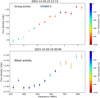 |
Fig. 3 Stokes V spectrum from imaging, (a) A 2 min averaged spectrum corresponding to the strongest flare F3. (b) A 51 min averaged spectrum during the for the weak activity period. |
4 Discussion
The high TB and polarisation fraction seen in the strong activity period suggest a coherent emission mechanism is at play, either via an ECME mechanism or a plasma emission process (see, Melrose 1993 for an overview). The following subsections summarise our current understanding of the two mechanisms.
4.1 Plasma emission
The coherent plasma emission mechanism can produce highly polarised emission (Tsytovich & Kaplan 1969; Melrose & Sy 1972). However, this mechanism is often subject to near-source scattering (e.g. Steinberg et al. 1971; Robinson 1983; Arzner & Magun 1999; Mohan et al. 2019; Kontar et al. 2019; Chen et al. 2020), which reduces the observed polarisation levels. In the case of solar type-III bursts, which are well-known plasma-emission sources, the maximum Stokes V/I detected is ≈60% (Saint-Hilaire et al. 2013; Rahman et al. 2020). However, these results are at frequencies below ≈100 MHz. Mohan (2021) showed that the effects of scattering could be less significant at higher frequencies since the effective scattering screen widths decrease towards higher frequency or equivalently at lower heights above the corona. This means that the scattering-induced depolarisation at our observing frequencies could be lower than that observed close to ≈ 100 MHz, but its effects may not be negligible. It is therefore unlikely that we observe radio bursts with polarisation levels above ≈75% generated purely via a coherent plasma emission mechanism.
4.2 Electron cyclotron maser emission
An ECME is driven by a loss-cone distribution of electrons. Such an unstable electron pitch-angle distribution can form in post-flare coronal loops (e.g. Wu & Lee 1979; Winglee & Dulk 1986; Ning et al. 2021). The ECME emission mechanism predicts that in νp/νB<0.3 X-mode (polarised in the sense of electron gyration), emission is dominant at fundamental νB. Recent studies using fully kinetic particle-in-cell simulations suggest that a harmonic X-mode emission via Z-mode coalescence can also form at νp/νB<0.3 and be observable (Ning et al. 2021). Meanwhile, in the 03<νp/νB<13 range, Z-mode emission at νB dominates (Melrose et al. 1984; Winglee 1985) with polarisation in the opposite sense of electron gyration (O-mode). However, X-mode emission at higher harmonics of νB can also form by the coalescence of Z-mode waves when there is a 0.3<νp/νB<1.3 regime (Melrose 1991). In a narrow window of 13<νp/νB<1.5, X-mode emission emitted directly at the harmonics of νB can be observed (Melrose et al. 1984). X-mode emission at harmonics of νB are expected via either a direct harmonic emission or various coalescence interactions up to νp/νB<3 (Bastian et al. 1990). Harmonics higher than three are hardly produced via any of these process due to the requirement of very high energy density in the unstable wave modes (Melrose 1991). So, 3νB is the highest observable harmonic expected. Another crucial factor is that the pure X-mode emission at νB, or an X-mode emission at harmonics of νB, formed by Z-mode coalescence can be nearly 100% polarised (Melrose 2009, 2017).
When νp/νB> 3, the emissivity of the various ECME processes drops dramatically, and along with the attenuation due to gyromagnetic absorption, ECME is expected to be insignificant (Melrose & Dulk 1982; Bastian 1990; Melrose 1991; Ning et al. 2021).
To summarise, the possible X-mode polarised ECME pathways driven by loss-cone electron distribution are as follows:
- 1.
νp/νB<0.3: fundamental emission at νB. Z-wave coalescence could produce emission observable at sνB (s = 2,3);
- 2.
0.3<νp/νB<13: Z or W wave coalescence can produce X-mode emission at sνB;
- 3.
1.3<νp/νB<3: harmonic X-mode emission at sνB via either a direct emission or wave coalescence interactions.
Beyond νp/νB=3, a plasma emission mechanism dominates. Ni et al. (2020) showed that when vp/νB >3, the Z, W, and UH modes triggered by an electron cyclotron maser instability would not escape the plasma. Instead, these waves can interact via a plasma emission mechanism to generate coherent emission at the fundamental and harmonic of the upper hybrid frequency,  .
.
Besides this, the existing ECME theory suggests that O-mode emission can be produced via the following pathway: 0.3<νp/νB<1.3: Z-mode pathway generates emission at νB.
4.3 The emission mechanism of AD Leo flares
In this subsection, we discuss the various possible mechanisms for the observed emission given the possible local physical scenarios during the various activity periods. First, we built 1D radial models of density and magnetic field for the star and used them to estimate νp and νB across coronal heights. Zeeman–Doppler imaging (ZDI) based studies (Morin et al. 2008; Bellotti et al. 2023) infer that the magnetic field of AD Leo is predominantly dipolar (>70%), with surface field strengths within ≈0.1–0.5 kG. However, the magnetic field strengths at strongly flaring active regions can be as high as 3kG (e.g. Cranmer & Saar 2011). Based on this, we chose a typical range for field strength at the base of the active region, Bfoot, between 0.3 and 1 kG. The chosen range considers a mean ZDI field strength at the lower end and the order of magnitude of the strongest reported active region IBI at the higher end. For the 1D analytical model of the radial magnetic field, two models are considered. The first one is a dipole-dominated active region magnetic field model suggested for solar active regions by Aschwanden et al. (1999):
 (1)
(1)
with the dipole scale height, hD, assumed to be 0.1 R* (R* is the stellar radius), based on solar studies (Aschwanden et al. 1999). We note that r is measured radially from stellar centre in units of R*. In the second model, we assume a simple multipole expansion model of magnetic field with the net magnetic flux assumed to be distributed as 72% dipole, 21% quadrupole, and 7% octapole fraction, based on the ZDI results for observations from 2020 (Bellotti et al. 2023):
 (2)
(2)
The fractional composition of the magnetic moments employed here are based on large-scale ZDI results that may not be representative of flaring active regions. Since no estimation of multipole moments at the stellar active region exists, we assume the large-scale fractional distribution. However, the high relative dipolar concentration in Eq. (2) assures that this is probably not an uncanny assumption for an active region’s magnetic structure if the AD Leo active regions are also similar to those of the Sun with strong bipolar magnetic field concentrations and arcade-like structures. The two models are referred to as Model 1 (Eq. (1)) and Model 2 (Eq. (2)) hereafter.
We derive vp(r) assuming the density model (ne(r)) proposed by Villadsen & Hallinan (2019):
 (3)
(3)
The basal coronal density in the model is derived from OVII line ratios by Ness et al. (2004). X-ray observations of pre-flare loops also suggest a basal coronal density within 1010–1011 cm−3 (Namekata et al. 2020). Meanwhile, the assumed radial density profile is empirical, but consistent with the best-fit hydrostatic equilibrium profiles derived for solar active regions based on direct measurements (e.g. Mann et al. 1999; Aschwanden et al. 2001). Zucca et al. (2014) showed that the data from a solar region that hosted a CME, is modelled well by an exponential hydrostatic equilibrium density profile for r ≲ 3R*, which is the height range of interest in our study.
Figure 4a shows the derived vp(r) and vB(r). The plotted range of vB(r) corresponds to 0.3≤ Bfoot ≤ 1 kG. The observing band (550–850 MHz) is marked in red. The green band shows the frequencies corresponding to one third of the observation band. For an ECME emission process, the observing frequency vobs = svB, where s = 1,2,3. First, we considered Model 1 (blue band). The region where the red band overlaps the blue one corresponds to the r range where vobs=vB. Similarly, the r range where the green band overlaps the blue one identifies the r range where vobs=3vB. Beyond this r range, the possibility of observing ECME in 500–850 MHz is very low since inherent emissivity drops significantly (Melrose et al. 1984). Vertical solid red lines mark the extent of the overlapping r range for vobs=vB, and the solid green lines mark the r range for vobs=3vB. The same exercise is performed for Model 2 (grey band). Instead of solid lines, we used dotted lines of the same colour to mark the r ranges.
Figure 4b shows the ratio vp/v for v = vB, vobs and vobs/3. Horizontal lines mark vp/vB=0.3, 1.3, and 3. We first consider Model 1. The overlap between the red and blue bands gives us the vp/vB values for the r range from where fundamental ECME mode emission can originate in the observing band. Clearly this ratio is greater than 1.3, but less than 3, implying that the fundamental X-mode emission is impossible, but a Z-mode ECME is possible. However, the polarisation will be in the opposite sense of electron gyration (O-mode). Moreover, an X-mode polarised emission is possible via the coalescence of Z or W waves, as per the standard theory (Melrose 1991). But the resultant harmonic X-mode emission would not be observable in our vobs band, but in the 2vobs band. Meanwhile, the overlap between green and blue bands gives us the vp/vB values in the r range from where, if third harmonic emission arises, it can be observed in our vobs. The range of vp/vB is much greater than 3, making an ECME emission mechanism unfavourable. Similar to the above discussion, for Model 2, the intersection between the grey and red bands gives the range of vp/vB for fundamental ECME emission, and the overlap between the grey and green bands gives the range of the ratio for harmonic emission to be observable in vobs band. If we consider the grey and red band overlap, we have cases for 0.3<vp/vB<3. Either an O or Z mode emission (0.3<vp/vB<1.3) or a harmonic X-mode (1.3<vp/vB<3) can be triggered here. However, akin to the case of Model 1, the harmonic X-mode emission born out of Z- or W-mode coalescence or a direct emission cannot be observed in our observing band. However, the overlap between the green (v =vobs/3) and grey bands falls within 1.3<v/vB<3, favouring a harmonic X-mode ECME from its r range via Z- or W-mode coalescence or a direct harmonic emission, which is observable in the vobs band.
To summarise , Model 1 only favours an O-mode polarised (opposite sense of electron gyration) emission at vB via a Z-mode pathway, which is observable in the vobs band. However, Model 2 favours an X-mode (polarised in the sense of electron gyration) emission at harmonics of local vB formed via either a direct emission or Z/W-mode coalescence pathways and observable in the vobs band.
We now consider the polarisation in the bursts to further constrain the mechanism. The polarisation has consistently been left circular with Stokes V/I > 60% during bursts. At higher frequencies (>700 MHz), we find higher polarisation degrees attained during strong flares (e.g. Fig. 3). Morin et al. (2008) had shown that the south pole of AD Leo is inclined well along the line of sight (LOS) at an angle of 20°. So, there is a high chance that magnetic field structures could be oriented southwards on the LOS. This means the observed emission is in the direction of electron gyration, which means the emission is in X-mode. Also, the degree of polarisation is >60% during flares, often reaching ≈100% at higher frequencies (see Fig. 3). If the emission is via an ECME process, the possible pathways are either a fundamental X-mode ECME mechanism from regions where vobs = vB or a harmonic X-mode emission from regions where vB= vobs/s and 0.3<vp/vB<3 (s = 2,3). Based on the inferences from Fig. 4, Model 1 does not favour both fundamental and harmonic X-mode ECME, but Model 2 favours a harmonic X-mode emission by all possible pathways. Meanwhile, Zhang et al. (2023) observed the star in the 1–1.5 GHz band during the strong activity period, from 21:13 to 22:48 UT, and reported emission features that are better explained by an ECME mechanism. Unfortunately, their observations did not extend further into the weak and quiescent activity phases.
Our analysis did not explicitly consider the propagation effects that would have affected the observed ECME. Without multi-waveband spectroscopic data, the existing stellar atmospheric models (e.g. Fontenla et al. 2016; Wedemeyer et al. 2013) cannot be well constrained to derive a reliable ambient/quiescent physical structure (especially B(r) and ne(r)), which is crucial to assessing the atmospheric opacity (see White & Kundu 1997; Treumann 2006). Consequently, based on current knowledge on the ECME mechanism as derived from solar observations, the emissivity should fall drastically above s = 2 (see Sect. 4.2). Moreover, the emission for higher harmonics (s = 2, 3) is less affected by gyromagnetic absorption from upper coronal layers (Zheleznyakov 1970; Melrose & Dulk 1982). Both of these strongly favour the detection of ECME at s = 2, 3. Our inferences on ECME generation based on 1D stellar models also favour harmonic emission.
Plasma emission, which is the competing mechanism to ECME, produces coherent emission observable at vp (F-branch) and 2vp (H-branch) (Ginzburg & Zhelezniakov 1958; Tsytovich & Kaplan 1969; Melrose & Sy 1972; Melrose 2009). This mechanism generally favours polarisation in the O-mode (Melrose 2017) especially for the F branch. For the H branch, this is true if vp>vB, but if vp/vB≲ 1.5, highly polarised X-mode emission at vobs = 2vp is possible (Willes & Melrose 1997). Given that we observe a high TB X-mode polarised flares, it is likely a H-branch emission from regions with vp/vB≲ 1.5. From Fig. 5b, we infer that the H-band emission observable in vobs should arise from r ≳ 1.9R*, where vp<vobs/2. In this r range, vp»vB for Model 1. However, for some Bfoot values, vp/vB<1.5 is satisfied for Model 2. So, only Model 2 can support an H-band plasma emission in X mode.
Based on the discussions so far, Model 2 favours X-mode polarised emission via both H-branch plasma emission mechanisms and ECME emission processes at harmonics of vB. We note that Model 1 does not support any of the likely emission processes favouring a strong X-mode ECME or H-band plasma emission. This possibly means that a solar-like active region model is not good for M dwarfs, but a ZDI-based multipole expansion model works better. For the rest of the discussion, we hence only consider Model 2. Meanwhile, the H-branch plasma emission observed in the Sun has always shown polarisation levels below 30% (Willes & Melrose 1997; Saint-Hilaire et al. 2013; Rahman et al. 2020). So, during a strong activity period, given the high polarisation of 60-100% (Figs. 1–3), the emission mechanism is likely via an ECME mechanism.
In the analysis so far, we had kept the basal coronal density constant in the model. We now consider a variation of this value within an order of magnitude and assess the possible ECME pathways supported by the two B(r) models. For this analysis, we vary ne within 1010–10n cm−3, consistent with the values reported by previous spectroscopic and X-ray continuum observations. This corresponds to a variation in the assumed basal coronal density in Eq. (3) by 0.4–4 times. If the basal density goes up four times, since  we would see an increase in vp by a factor of two, which in turn raises all the vp/v bands in Fig. 4 by the same factor. We note that in Fig. 4 the green band overlaps with the grey one (Model 2) within 1 <vp/v < 3. So, the harmonic X-mode ECME emission pathway, previously supported by Model 2, will remain feasible, but now in the 2<vp/v < 3. The other ECME pathways that were already not supported by the previously assumed lower density plasma will be unsupported by a denser plasma due to enhanced damping of the ECME driving instability. However, since vobs/3 overlaps with Model 2 in vp/v < 10, an ECME-driven coherent plasma emission process suggested by Ni et al. (2020) can produce harmonic X-mode emission observable in vobs. Meanwhile, if we assume a 0.4 times lower density in the active region, all the vp/v bands in Fig. 4 will be reduced by a factor of 1.6. In this case for Model 2, harmonic X-mode emission will be observable as before. Interestingly, a portion of the overlapping region between Model 1 (blue band) and the green band will fall within 2.5<vp/v < 3, suggesting a possibility of observing a harmonic X-mode emission in vobs. This may make Model 1 viable for a small range of Bfoot and basal density values. However, Model 2 consistently supports an ECME mechanism for an order of magnitude range of Bfoot and ne values.
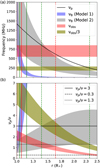 |
Fig. 4 Possible scenarios for ECME mechanism to operate, (a) vp(r) and vB(r) for corona of AD Leo. vB is found using Model 1 (Eq. (1)) and Model 2 (Eq. (2)). The observing band (vobs ∊ [550, 850] MHz) and vobs/3 are marked, (b) vp/vB(r) for two B(r) models and the ratios of vp to v for vobs and vobs/3 are shown. Colour choice is the same as in the top panel. Red lines mark the r range where vobs overlap vB and green lines mark the overlap r range of vobs/3 with vB (solid line: Model 1, dashed: Model 2). |
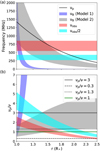 |
Fig. 5 Possible scenarios for plasma emission mechanism to operate, (a) Blue, red, and grey bands are the same as in Fig. 4. Cyan region marks vobs/2 band, (b) vp/vB(r) and vp/vobs ratio as in Fig. 4b. Cyan band shows vp/v for vobs/2. |
4.4 Weak activity period and the type-IV burst
The post-flare weak activity phase is found to last for ≈ 1.4 h. The Stokes V dynamic spectrum (Fig. 1a) shows that the post-flare emission shows a bright patch confined to frequencies ≳700MHz, between 2021-12-03 23:27 and 2021-12-04 02:25 UT. To highlight this better, a 200 s averaged VISAD spectrum was made (see Fig. 6a). The imaging-based spectrum from the weak activity period (Fig. 3b) also shows a characteristic high-polarisation bright-emission feature above ≈700–730 MHz, where the emission polarisation jumps above ≈55% and rises to ≈80% as frequency increases. As per the solar radio burst classification scheme, the aforementioned features suggest that the weak activity phase corresponds to a type-IV radio burst confined to frequencies above 700 MHz (Gopalswamy 2011; Hillaris et al. 2016; Salas-Matamoros & Klein 2020). For comparison, Fig. 6b shows a solar dynamic spectrum during a strong CME taken by the Wind/WAVES instrument. The solar data are taken from the publicly available type-IV catalogue compiled by Coordinated Data Analysis Workshops (CDAW) data centre3. The solar event was so chosen to match the dynamic spectral emission profile of the AD Leo. The morphological analogues of the type-III and type-IV bursts in the solar template spectrum can be identified in the AD Leo DS.
Type-IV radio bursts are associated with strong flares and CMEs in the Sun, as the sought-after type-II bursts (Robinson 1986; Gopalswamy 2011; Hillaris et al. 2016; Kumari et al. 2021). While a type-II burst is associated with the coronal shock generated by a fast CME, a type-IV burst is generated by flare-accelerated electrons trapped either in the post-flare loops or in the moving plasmoids associated with the CME (e.g. Wild 1970; Smerd 1970; Gopalswamy et al. 2005; White 2007; Gopalswamy 2011). Type-IVs are generally associated with relatively longer and stronger solar X-ray flares than type-IIs (Cane & Reames 1988). Also, type-IV bursts are often linked to strong CMEs, which expand out to heliocentric angular widths >60°, with mean speeds >900 km s−1 (Robinson 1986; Gopalswamy 2011; Hillaris et al. 2016). Recently, Zic et al. (2020) reported the first type-IV burst detection in a star other than the Sun, namely Proxima Centauri, which is an old (≈5 Gyr) M dwarf. Given its age (≈ 250 Myr) and rotation period (Prot = 2.2 days), AD Leo belongs to a fast rotating (period <5 days), young (age <1 Gyr) and more active stellar population (‘C’ branch) compared to the Sun (age = 4.6 Gyr; Prot = 25 days), which belongs to the less active ‘I’ branch stars (Barnes 2003; Brown 2014). Barnes (2003) demonstrated that the stars undergo an evolutionary migration from ‘C’ to ‘I’ branch as they spin down with age due to mass and angular momentum loss. This migration involves a fundamental change in the way the internal dynamo couples with the external active atmospheric layers and the stellar wind (Brown 2014; Garraffo et al. 2018). So, though Proxima Centauri is an M dwarf, it is an ‘I’ branch star, but AD Leo is not. Here, we report the first detection of a type-IV burst on a young (≈250 Myr), active ‘C’ branch M dwarf.
We do not find evidence of a type-II burst, making it still elusive in an M dwarf despite monitoring campaigns spanning several days on various stars, including AD Leo (e.g. Osten & Bastian 2008; Villadsen & Hallinan 2019). Though rare, solar type-II bursts have also been found to be associated with coronal shocks produced by failed eruptions, unrelated to CMEs (e.g. Magdalenic et al. 2012; Morosan et al. 2023). AD Leo is an active star with a magnetic field that is an order of magnitude stronger and predominantly axi-symmetric (Moschou et al. 2019). Theoretical models have argued that the strong magnetic field structures and the associated high Alfvén speed barriers in the stellar corona could either block even the energetic flares from causing a CME (failed eruption scenario), or resist the formation of a strong shock required to initiate a type-II emission during an eruption/CME (Odert et al. 2020; Alvarado-Gómez et al. 2022). This means that, unlike the case of the Sun, AD Leo could host more failed eruptions during strong flares, and even if a CME or eruption occurs, type-II bursts need not be triggered for most events. These scenarios can explain why there have been no reports of a type-II burst on AD Leo despite several monitoring campaigns (e.g. Osten & Bastian 2006, 2008; Villadsen & Hallinan 2019). In any case, since post-flare loop structures will trap flare-accelerated electrons, strong type-IV bursts could trace CMEs better than type-IIs in M dwarfs.
Given the high X-mode polarisation level, high TB at vobs≳ 700 MHz, and our inferences for the active region in the previous section, the type-IV burst emission likely originates from an ECME mechanism via either a Z/W-mode coalescence or a harmonic emission pathway. An ECME mechanism is usually triggered by an unstable loss-cone distribution of energetic electrons formed within a magnetic bottle-like configuration, readily provided by the post-flare loops (e.g. Carley et al. 2019). In the case of the Sun, type-IV bursts are generally associated with plasma emission mechanism in the metric waveband (Weiss 1963; Salas-Matamoros & Klein 2020). However, during some strong flares, associated type-IV bursts have demonstrated ≈ millisecond to second scale spiky emission features in their dynamic spectra with high degrees of circular polarisation and TB, often modelled as generated by an ECME mechanism (e.g. Carley et al. 2019; Liu et al. 2018; Morosan et al. 2019; Cliver et al. 2022). Certain high time-resolution studies of AD Leo in 1–3 GHz observations have reported ≈ms scale spiky emission features (e.g. Osten & Bastian 2008; Zhang et al. 2023). The time resolution of uGMRT data restricts us from exploring sub-second-scale fine structures in the dynamic spectrum. The ECME signatures we detect in the type-IV emission above 700 MHz could probably be formed by numerous sub-second-scale fine structures. Meanwhile, at frequencies below 700 MHz the emission polarisation is well below 30%. The emission mechanism here is likely a H-branch plasma emission, which is known to produce high TB emission at low polarisation levels (e.g. Willes & Melrose 1997; Saint-Hilaire et al. 2013; Rahman et al. 2019).
Since the type-IV emission is seen to be mostly confined within 700 MHz (Fig. 6), using Model 2 and assuming that the ECME is formed at either the second or the third harmonic of νB, the height of the post flare loop can be inferred. It can be seen from Fig. 5b that within 1.8~2.25 R*, the overlap region of the cyan and grey bands satisfy the condition of 0.3<νp/νB<1.5 required for Z-mode or harmonic X-mode mechanism to operate efficiently and produce a second harmonic ECME observable in νobs. Since 700 MHz is roughly the centre of the cyan band, the post-flare loop height could be ≈ 1.8–2.0 R*. Similarly, if the emission is at the third harmonic (νobs= 3νB), we should use Figs. 4a,b to obtain emission height. Here, instead of the cyan band, we considered the overlap between the green and the grey bands. The emission height range turns out to be ≈2.0–2.5 R*, implying a post-flare loop height of ≈2–2.25 R*. This implies that the star can have loops rising to about 1 R* above the photosphere.
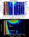 |
Fig. 6 Comparison between AD Leo DS and a typical solar DS during a CME. (a) AD Leo VISAD spectrum with 200 s and 10 MHz averaging with a saturated colour scale. (b) A solar radio spectrum from Wind/WAVES instrument showing the different burst types associated with a solar CME on Jan 4, 2004. Solar type-IV and type-III features can be identified in the AD Leo spectrum. Solar data credit: CDAW data centre. |
4.5 Quasi-steady period
The quiescent Stokes I flux level varies within ≈ 1–1.75 mJy (see Figs. 1c and 2), implying TB values of the order of ≈1010 K. However, the polarisation levels of ≈20–30% inferred from the light curve suggests a H-band coherent plasma emission mechanism. The observed emission is likely a superposition of various spatially separated coherent plasma emission regions or a mixture of gyrosynchroton and plasma emission regions (Bastian et al. 1990; Bastian 1994).
5 Conclusions
We present a 2-h-long metric band flaring activity in a young active M dwarf, AD Leo. A hydrostatic equilibrium electron density profile was assumed with a basal density ranging within 1010–1011 cm−3. Based on the existing knowledge on the stellar magnetic field, different radial profiles (B(r)) were considered: a solar-like model and a simple multipole expansion model. Contrasting the radio data with these models, we conclude the following:
The active region B(r) is more consistent with a multipole expansion model than a solar-like model, given the possible range of magnetic field strength and density at the base of the corona;
The observed radio bursts are powered by an ECME mechanism.
The period of strong flaring was succeeded by a post-flare activity period. We report a solar-like type-IV radio burst in AD Leo, in the post-flare phase, characterised by a distinctive dynamic spectral morphology and circular polarisation levels ranging from 60% to 100%. Previously, a type-IV emission was reported in Proxima Centauri by Zic et al. (2020). This is the first solarlike type-IV detection on a young active M dwarf belonging to a different age-activity population (‘C’ branch) relative to the Sun (belonging to ‘I’ branch) (Barnes 2003). The emission characteristics favour an ECME mechanism at the second or third harmonic of the local gyrofrequency. The detection of the type-IV burst could signify a strong CME, since solar type-IVs are known to be associated with fast and wide CMEs. Nevertheless, an hour-long type-IV burst signifies powerful accelerated particle activity in the post-flare loops. Based on the frequency extent of the type-IV burst in the VISAD dynamic spectrum, we infer that the post-flare loops could rise up to ≈ 1 R* scales above photosphere into the inter-planetary space. The quasi-steady emission that followed the type-IV activity is likely powered by a mixture of several coherent plasma emission regions.
Acknowledgements
This work is supported by the Research Council of Norway through the EMISSA project (project number 286853) and the Centres of Excellence scheme, project number 262622 (“Rosseland Centre for Solar Physics”). We thank the staff of the GMRT that made these observations possible. GMRT is run by the National Centre for Radio Astrophysics of the Tata Institute of Fundamental Research. This research made use of NASA’s Astrophysics Data System (ADS). AM and NG are supported in part by NASA’s STEREO project and LWS program. AM acknowledges the developers of the various Python modules namely Numpy (Harris et al. 2020), Astropy (Astropy Collaboration 2013), Matplotlib (Hunter 2007) and multiprocessing. AM also thanks the developers of CASA (McMullin et al. 2007). AM acknowledges the discussions with Barnali Das which greatly helped speed up the data analysis. AM acknowledges the discussions with Tim Bastian.
References
- Alvarado-Gómez, J. D., Drake, J. J., Cohen, O., et al. 2022, Astron. Nachr., 343, e10100 [Google Scholar]
- Arzner, K., & Magun, A. 1999, A&A, 351, 1165 [NASA ADS] [Google Scholar]
- Aschwanden, M. J., Newmark, J. S., Delaboudinière, J.-P., et al. 1999, ApJ, 515, 842 [CrossRef] [Google Scholar]
- Aschwanden, M. J., Schrijver, C. J., & Alexander, D. 2001, ApJ, 550, 1036 [NASA ADS] [CrossRef] [Google Scholar]
- Astropy Collaboration (Robitaille, T. P., et al.) 2013, A&A, 558, A33 [NASA ADS] [CrossRef] [EDP Sciences] [Google Scholar]
- Barnes, S. A. 2003, ApJ, 586, 464 [Google Scholar]
- Bashi, D., Zucker, S., Adibekyan, V., et al. 2020, A&A, 643, A106 [NASA ADS] [CrossRef] [EDP Sciences] [Google Scholar]
- Bastian, T. S. 1990, Sol. Phys., 130, 265 [NASA ADS] [CrossRef] [Google Scholar]
- Bastian, T. S. 1994, Space Sci. Rev., 68, 261 [NASA ADS] [CrossRef] [Google Scholar]
- Bastian, T. J. 1996, in Radio Emission from the Stars and the Sun, eds. A. R. Taylor, & J. M. Paredes, Astronomical Society of the Pacific Conference Series, 93, 447 [NASA ADS] [Google Scholar]
- Bastian, T. S., Bookbinder, J., Dulk, G. A., & Davis, M. 1990, ApJ, 353, 265 [NASA ADS] [CrossRef] [Google Scholar]
- Bellotti, S., Morin, J., Lehmann, L. T., et al. 2023, A&A, 676, A56 [NASA ADS] [CrossRef] [EDP Sciences] [Google Scholar]
- Benz, A. O. 1996, in Radio Emission from the Stars and the Sun, eds. A. R. Taylor, & J. M. Paredes, Astronomical Society of the Pacific Conference Series, 93, 347 [NASA ADS] [Google Scholar]
- Brown, T. M. 2014, ApJ, 789, 101 [Google Scholar]
- Cairns, I. H., & Melrose, D. B. 1985, J. Geophys. Res., 90, 6637 [NASA ADS] [CrossRef] [Google Scholar]
- Callingham, J. R., Shimwell, T. W., Vedantham, H. K., et al. 2023, A&A, 670, A124 [NASA ADS] [CrossRef] [EDP Sciences] [Google Scholar]
- Cane, H. V., & Reames, D. V. 1988, ApJ, 325, 895 [NASA ADS] [CrossRef] [Google Scholar]
- Carleo, I., Malavolta, L., Lanza, A. F., et al. 2020, A&A, 638, A5 [NASA ADS] [CrossRef] [EDP Sciences] [Google Scholar]
- Carley, E. P., Hayes, L. A., Murray, S. A., et al. 2019, Nat. Commun., 10, 2276 [NASA ADS] [CrossRef] [Google Scholar]
- CASA Team (Bean, B., et al.) 2022, PASP, 134, 114501 [NASA ADS] [CrossRef] [Google Scholar]
- Chen, X., Kontar, E. P., Chrysaphi, N., et al. 2020, ApJ, 905, 43 [NASA ADS] [CrossRef] [Google Scholar]
- Cliver, E. W., Schrijver, C. J., Shibata, K., & Usoskin, I. G. 2022, LRSP, 19, 2 [NASA ADS] [Google Scholar]
- Cornwell, T., & Fomalont, E. B. 1999, in Synthesis Imaging in Radio Astronomy II, eds. G. B. Taylor, C. L. Carilli, & R. A. Perley, Astronomical Society of the Pacific Conference Series, 180, 187 [NASA ADS] [Google Scholar]
- Cranmer, S. R., & Saar, S. H. 2011, ApJ, 741, 54 [Google Scholar]
- Crespo-Chacón, I., Montes, D., García-Alvarez, D., et al. 2006, A&A, 452, 987 [NASA ADS] [CrossRef] [EDP Sciences] [Google Scholar]
- Dal, H. 2020, MNRAS, 495, 4529 [NASA ADS] [CrossRef] [Google Scholar]
- Das, B., Kudale, S., Chandra, P., et al. 2020, arXiv e-prints, [arXiv:2004.08542] [Google Scholar]
- Donati, J. F., & Landstreet, J. D. 2009, ARA&A, 47, 333 [Google Scholar]
- Dulk, G. A. 1985, ARA&A, 23, 169 [Google Scholar]
- Dulk, G. A., & Winglee, R. M. 1987, Sol. Phys., 113, 187 [CrossRef] [Google Scholar]
- Enßlin, T. A., Hutschenreuter, S., Vacca, V., & Oppermann, N. 2017, Phys. Rev. D, 96, 043021 [CrossRef] [Google Scholar]
- Fontenla, J. M., Linsky, J. L., Garrison, J., et al. 2016, ApJ, 830, 154 [NASA ADS] [CrossRef] [Google Scholar]
- Garraffo, C., Drake, J. J., Dotter, A., et al. 2018, ApJ, 862, 90 [NASA ADS] [CrossRef] [Google Scholar]
- Gergely, T. E. 1986, Sol. Phys., 104, 175 [Google Scholar]
- Ginzburg, V. L., & Zhelezniakov, V. V. 1958, Soviet Ast., 2, 653 [NASA ADS] [Google Scholar]
- Gopalswamy, N. 2011, in Planetary, Solar and Heliospheric Radio Emissions (PRE VII), eds. H. O. Rucker, W. S. Kurth, P. Louarn, & G. Fischer, 325 [CrossRef] [Google Scholar]
- Gopalswamy, N., Aguilar-Rodriguez, E., Yashiro, S., et al. 2005, J. Geophys. Res. Space Phys., 110, A12S07 [NASA ADS] [Google Scholar]
- Güdel, M. 2002, ARA&A, 40, 217 [Google Scholar]
- Gupta, Y., Ajithkumar, B., Kale, H. S., et al. 2017, Curr. Sci., 113, 707 [NASA ADS] [CrossRef] [Google Scholar]
- Harris, C. R., Millman, K. J., van der Walt, S. J., et al. 2020, Nature, 585, 357 [NASA ADS] [CrossRef] [Google Scholar]
- Hillaris, A., Bouratzis, C., & Nindos, A. 2016, Sol. Phys., 291, 2049 [NASA ADS] [CrossRef] [Google Scholar]
- Hunter, J. D. 2007, Comput. Sci. Eng., 9, 90 [NASA ADS] [CrossRef] [Google Scholar]
- Kontar, E. P., Chen, X., Chrysaphi, N., et al. 2019, ApJ, 884, 122 [NASA ADS] [CrossRef] [Google Scholar]
- Kumari, A., Morosan, D. E., & Kilpua, E. K. J. 2021, ApJ, 906, 79 [Google Scholar]
- Liu, H., Chen, Y., Cho, K., et al. 2018, Sol. Phys., 293, 58 [NASA ADS] [CrossRef] [Google Scholar]
- Lund, K., Jardine, M., Lehmann, L. T., et al. 2020, MNRAS, 493, 1003 [NASA ADS] [CrossRef] [Google Scholar]
- Macquart, J. P., & Melrose, D. B. 2000, ApJ, 545, 798 [NASA ADS] [CrossRef] [Google Scholar]
- Magdalenic, J., Marqué, C., Zhukov, A. N., Vrsnak, B., & Veronig, A. 2012, ApJ, 746, 152 [NASA ADS] [CrossRef] [Google Scholar]
- Mann, G., Jansen, F., MacDowall, R. J., Kaiser, M. L., & Stone, R. G. 1999, A&A, 348, 614 [NASA ADS] [Google Scholar]
- McLean, D., & Labrum, N. 1985, Solar Radio Astrophysics (Cambridge University Press) [Google Scholar]
- McMullin, J. P., Waters, B., Schiebel, D., Young, W., & Golap, K. 2007, in Astronomical Data Analysis Software and Systems XVI, eds. R. A. Shaw, F. Hill, & D. J. Bell, Astronomical Society of the Pacific Conference Series, 376, 127 [Google Scholar]
- Melrose, D. B. 1991, ApJ, 380, 256 [NASA ADS] [CrossRef] [Google Scholar]
- Melrose, D. B. 1993, PASA, 10, 254 [NASA ADS] [CrossRef] [Google Scholar]
- Melrose, D. B. 2009, ArXiv e-prints [arXiv:0902.2034] [Google Scholar]
- Melrose, D. B. 2017, Rev. Modern Plasma Phys., 1, 5 [NASA ADS] [CrossRef] [Google Scholar]
- Melrose, D. B., & Dulk, G. A. 1982, ApJ, 259, 844 [Google Scholar]
- Melrose, D. B., & Sy, W. N. 1972, Aust. J. Phys., 25, 387 [NASA ADS] [CrossRef] [Google Scholar]
- Melrose, D. B., Hewitt, R. G., & Dulk, G. A. 1984, J. Geophys. Res., 89, 897 [CrossRef] [Google Scholar]
- Mohan, A. 2021, A&A, 655, A77 [NASA ADS] [CrossRef] [EDP Sciences] [Google Scholar]
- Mohan, A., Mondal, S., Oberoi, D., & Lonsdale, C. J. 2019, ApJ, 875, 98 [NASA ADS] [CrossRef] [Google Scholar]
- Morin, J., Donati, J. F., Petit, P., et al. 2008, MNRAS, 390, 567 [Google Scholar]
- Morosan, D. E., Kilpua, E. K. J., Carley, E. P., & Monstein, C. 2019, A&A, 623, A63 [NASA ADS] [CrossRef] [EDP Sciences] [Google Scholar]
- Morosan, D. E., Pomoell, J., Kumari, A., Kilpua, E. K. J., & Vainio, R. 2023, A&A, 675, A98 [NASA ADS] [CrossRef] [EDP Sciences] [Google Scholar]
- Moschou, S.-P., Drake, J. J., Cohen, O., et al. 2019, ApJ, 877, 105 [NASA ADS] [CrossRef] [Google Scholar]
- Namekata, K., Maehara, H., Sasaki, R., et al. 2020, PASJ, 72, 68 [NASA ADS] [CrossRef] [Google Scholar]
- Ness, J. U., Güdel, M., Schmitt, J. H. M. M., Audard, M., & Telleschi, A. 2004, A&A, 427, 667 [NASA ADS] [CrossRef] [EDP Sciences] [Google Scholar]
- Ni, S., Chen, Y., Li, C., et al. 2020, ApJ, 891, L25 [NASA ADS] [CrossRef] [Google Scholar]
- Ning, H., Chen, Y., Ni, S., et al. 2021, ApJ, 920, L40 [NASA ADS] [CrossRef] [Google Scholar]
- Odert, P., Leitzinger, M., Guenther, E. W., & Heinzel, P. 2020, MNRAS, 494, 3766 [NASA ADS] [CrossRef] [Google Scholar]
- Osten, R. A., & Bastian, T. S. 2006, ApJ, 637, 1016 [NASA ADS] [CrossRef] [Google Scholar]
- Osten, R. A., & Bastian, T. S. 2008, ApJ, 674, 1078 [NASA ADS] [CrossRef] [Google Scholar]
- Rahman, M. M., McCauley, P. I., & Cairns, I. H. 2019, Sol. Phys., 294, 7 [CrossRef] [Google Scholar]
- Rahman, M. M., Cairns, I. H., & McCauley, P. I. 2020, Sol. Phys., 295, 51 [NASA ADS] [CrossRef] [Google Scholar]
- Robinson, R. D. 1983, PASA, 5, 208 [NASA ADS] [CrossRef] [Google Scholar]
- Robinson, R. D. 1986, Sol. Phys., 104, 33 [NASA ADS] [CrossRef] [Google Scholar]
- Saikia, D. J., & Salter, C. J. 1988, ARA&A, 26, 93 [NASA ADS] [CrossRef] [Google Scholar]
- Saint-Hilaire, P., Vilmer, N., & Kerdraon, A. 2013, ApJ, 762, 60 [NASA ADS] [CrossRef] [Google Scholar]
- Salas-Matamoros, C., & Klein, K.-L. 2020, A&A, 639, A102 [EDP Sciences] [Google Scholar]
- Smerd, S. F. 1970, PASA, 1, 305 [Google Scholar]
- Spangler, S. R., Rankin, J. M., & Shawhan, S. D. 1974, ApJ, 194, L43 [NASA ADS] [CrossRef] [Google Scholar]
- Steinberg, J. L., Aubier-Giraud, M., Leblanc, Y., & Boischot, A. 1971, A&A, 10, 362 [NASA ADS] [Google Scholar]
- Treumann, R. A. 2006, A&A Rev, 13, 229 [CrossRef] [Google Scholar]
- Tsytovich, V. N., & Kaplan, S. A. 1969, Soviet Ast., 12, 618 [NASA ADS] [Google Scholar]
- Tuomi, M., Jones, H. R. A., Barnes, J. R., et al. 2018, AJ, 155, 192 [NASA ADS] [CrossRef] [Google Scholar]
- van den Besselaar, E. J. M., Raassen, A. J. J., Mewe, R., et al. 2003, A&A, 411, 587 [NASA ADS] [CrossRef] [EDP Sciences] [Google Scholar]
- Vedantham, H. K. 2021, MNRAS, 500, 3898 [Google Scholar]
- Vidotto, A. A., Gregory, S. G., Jardine, M., et al. 2014, MNRAS, 441, 2361 [Google Scholar]
- Villadsen, J., & Hallinan, G. 2019, ApJ, 871, 214 [Google Scholar]
- Wedemeyer, S., Ludwig, H. G., & Steiner, O. 2013, Astron. Nachr., 334, 137 [NASA ADS] [CrossRef] [Google Scholar]
- Weiss, A. A. 1963, Aust. J. Phys., 16, 526 [NASA ADS] [CrossRef] [Google Scholar]
- White, S. 2007, Asian J. Phys, 16, 189 [Google Scholar]
- White, S. M., & Kundu, M. R. 1997, Sol. Phys., 174, 31 [NASA ADS] [CrossRef] [Google Scholar]
- White, S. M., Jackson, P. D., & Kundu, M. R. 1989, ApJS, 71, 895 [Google Scholar]
- Wild, J. P. 1970, PASA, 1, 365 [NASA ADS] [CrossRef] [Google Scholar]
- Willes, A. J., & Melrose, D. B. 1997, Sol. Phys., 171, 393 [NASA ADS] [CrossRef] [Google Scholar]
- Winglee, R. M. 1985, in Radio Stars, eds. R. M. Hjellming, & D. M. Gibson, Astrophysics and Space Science Library, 116, 49 [NASA ADS] [CrossRef] [Google Scholar]
- Winglee, R. M., & Dulk, G. A. 1986, ApJ, 307, 808 [Google Scholar]
- Wu, C. S., & Lee, L. C. 1979, ApJ, 230, 621 [Google Scholar]
- Zaitsev, V. V., Kruger, A., Hildebrandt, J., & Kliem, B. 1997, A&A, 328, 390 [NASA ADS] [Google Scholar]
- Zhang, J., Tian, H., Zarka, P., et al. 2023, ApJ, 953, 65 [NASA ADS] [CrossRef] [Google Scholar]
- Zheleznyakov, V. V. 1970, Radio emission of the sun and planets (Oxford: Pergamon Press) [Google Scholar]
- Zic, A., Murphy, T., Lynch, C., et al. 2020, ApJ, 905, 23 [Google Scholar]
- Zucca, P., Carley, E. P., Bloomfield, D. S., & Gallagher, P. T. 2014, A&A, 564, A47 [NASA ADS] [CrossRef] [EDP Sciences] [Google Scholar]
All Figures
|
Fig. 1 Results from VISAD pipeline. (a) Stokes V dynamic spectrum. (b, c) Band-averaged light curves in Stokes V and I. The ordinate shows TB (left) and flux density (right), respectively. Different periods of activity are marked. Basal flux density levels in Stokes I and V are represented by dotted lines in the respective panels. We note that the TB values are nominal and simply highlight that the emission is via a coherent emission mechanism. Since the true source sizes are unknown, an average (i.e. across the whole unresolved stellar disc) TB is computed here. |
| In the text | |
|
Fig. 2 Band-averaged Stokes I and V light curves obtained from imaging analysis. The detections below 5σ are marked as upper limits. Transparent squares mark poor polarisation estimates. |
| In the text | |
|
Fig. 3 Stokes V spectrum from imaging, (a) A 2 min averaged spectrum corresponding to the strongest flare F3. (b) A 51 min averaged spectrum during the for the weak activity period. |
| In the text | |
|
Fig. 4 Possible scenarios for ECME mechanism to operate, (a) vp(r) and vB(r) for corona of AD Leo. vB is found using Model 1 (Eq. (1)) and Model 2 (Eq. (2)). The observing band (vobs ∊ [550, 850] MHz) and vobs/3 are marked, (b) vp/vB(r) for two B(r) models and the ratios of vp to v for vobs and vobs/3 are shown. Colour choice is the same as in the top panel. Red lines mark the r range where vobs overlap vB and green lines mark the overlap r range of vobs/3 with vB (solid line: Model 1, dashed: Model 2). |
| In the text | |
|
Fig. 5 Possible scenarios for plasma emission mechanism to operate, (a) Blue, red, and grey bands are the same as in Fig. 4. Cyan region marks vobs/2 band, (b) vp/vB(r) and vp/vobs ratio as in Fig. 4b. Cyan band shows vp/v for vobs/2. |
| In the text | |
|
Fig. 6 Comparison between AD Leo DS and a typical solar DS during a CME. (a) AD Leo VISAD spectrum with 200 s and 10 MHz averaging with a saturated colour scale. (b) A solar radio spectrum from Wind/WAVES instrument showing the different burst types associated with a solar CME on Jan 4, 2004. Solar type-IV and type-III features can be identified in the AD Leo spectrum. Solar data credit: CDAW data centre. |
| In the text | |
Current usage metrics show cumulative count of Article Views (full-text article views including HTML views, PDF and ePub downloads, according to the available data) and Abstracts Views on Vision4Press platform.
Data correspond to usage on the plateform after 2015. The current usage metrics is available 48-96 hours after online publication and is updated daily on week days.
Initial download of the metrics may take a while.