| Issue |
A&A
Volume 686, June 2024
|
|
|---|---|---|
| Article Number | A87 | |
| Number of page(s) | 11 | |
| Section | Astrophysical processes | |
| DOI | https://doi.org/10.1051/0004-6361/202347828 | |
| Published online | 03 June 2024 | |
Repeating X-ray bursts: Interaction between a neutron star and clumps partially disrupted from a planet
1
Xinjiang Astronomical Observatory, Chinese Academy of Sciences, Urumqi, 830011 Xinjiang, PR China
e-mail: akurban@xao.ac.cn; na.wang@xao.ac.cn; zhouxia@xao.ac.cn
2
Key Laboratory of Radio Astronomy, Chinese Academy of Sciences, Urumqi, 830011 Xinjiang, PR China
3
Xinjiang Key Laboratory of Radio Astrophysics, Urumqi, 830011 Xinjiang, PR China
4
School of Astronomy and Space Science, Nanjing University, Nanjing 210023, PR China
5
Key Laboratory of Modern Astronomy and Astrophysics (Nanjing University), Ministry of Education, Nanjing 210023, PR China
6
School of Physics and Electronic Engineering, Sichuan University of Science & Engineering, Zigong 643000, PR China
Received:
30
August
2023
Accepted:
12
March
2024
Repeating X-ray bursts from the Galactic magnetar SGR 1806-20 have been observed with a period of 398 days. Similarly, periodic X-ray bursts from SGR 1935+2154 with a period of 238 days have also been observed. Here we argue that these X-ray bursts could be produced by the interaction of a neutron star (NS) with its planet in a highly elliptical orbit. The periastron of the planet is very close to the NS, so it would be partially disrupted by the tidal force every time it passes through the periastron. Major fragments generated in the process will fall onto the NS under the influence of gravitational perturbation. The collision of the in-falling fragments with the NS produces repeating X-ray bursts. The main features of the observed X-ray bursts, such as their energy, duration, periodicity, and activity window, can all be explained in our framework.
Key words: planet-star interactions / stars: neutron / X-rays: bursts
© The Authors 2024
 Open Access article, published by EDP Sciences, under the terms of the Creative Commons Attribution License (https://creativecommons.org/licenses/by/4.0), which permits unrestricted use, distribution, and reproduction in any medium, provided the original work is properly cited.
This article is published in open access under the Subscribe to Open model. Subscribe to A&A to support open access publication.
1. Introduction
Magnetars are highly magnetized neutron stars (NSs; Thompson & Duncan 1995) that are characterized by recurrent emission of short-duration bursts (a few milliseconds to seconds) in soft γ-rays and/or hard X-rays, with burst energies in the range 1035–1046 erg (see the review articles Turolla et al. 2015 and Kaspi & Beloborodov 2017 and reference therein). More than 30 magnetars have been observed to date,1 and they show diverse burst properties (Olausen & Kaspi 2014).
Many models have been proposed to account for magnetar burst activities. According to their energy sources, these models can be divided into two categories: internal and external mechanisms. In the internal mechanism models, the burst energy mainly comes from the magnetic field, whose decay leads to a rupture of the crust and rapid magnetic reconnection, which releases a large amount of energy and causes particle acceleration and radiation in the magnetosphere (Thompson & Duncan 1995; Lyutikov 2003; Gill & Heyl 2010; Turolla et al. 2015).
On the other hand, in the external mechanism models, the energy comes from the interaction between the compact stars – for example NSs or strange stars (SSs) – and external material. The bursts could also be due to the impact of massive comet-like objects with a NS (Katz 1996; Chatterjee et al. 2000; Marsden et al. 2001) or a SS (Zhang et al. 2000; Usov 2001; Ouyed et al. 2011). We note that in the models the origin and location of these small bodies can be different. They can come from a fossil disk formed after the birth of the NS and/or SS (Chatterjee et al. 2000; Marsden et al. 2001) or from the comet clouds around the central star (like the Oort cloud in the Solar System; Zhang et al. 2000). They can even be formed during a quark nova explosion, an explosive phenomenon that happens when a NS is converted into a SS due to spin-down or accretion processes (Ouyed et al. 2011). We note that both NSs and SSs could be involved in the bursts and super-Eddington activities (e.g., Katz 1996; Geng et al. 2021).
At present, it is not clear which of the various mechanisms is in operation. The richness of the phenomenology indicates that a combination of mechanisms are responsible (Turolla et al. 2015).
Recent studies show that two soft gamma-ray repeaters (SGRs), SGR 1806-20 and SGR 1935+2154, may have periodic burst activities. SGR 1806-20 was initially known as GB790107 and was identified as a gamma-ray repeater by Laros et al. (1986). It has a surface magnetic field of B⋆ = 2 × 10¹⁵ G (Olausen & Kaspi 2014) and a spin period of Pspin = 7.55 s (Woods et al. 2007). Zhang et al. (2021a) analyzed the arrival time of more than 3000 short bursts from SGR 1806-20 detected by different telescopes (Göǧüş et al. 2000; Prieskorn & Kaaret 2012; Kırmızıbayrak et al. 2017) and found a possible period of about 398 days for the source.
SGR 1935+2154 was discovered by Stamatikos et al. (2014). The surface magnetic field of this source is B⋆ = 2.2 × 10¹⁴ G, and the spin period is Pspin = 3.245 s (Israel et al. 2016). After analyzing the arrival time of more than 300 X-ray bursts from SGR 1935+2154, Zou et al. (2021) argued that these bursts exhibit a period of ∼238 days, with a 150 days active window (63.3% of the period). However, Xie et al. (2022) revisited the periodicity of SGR 1935+2154 with an updated sample and found the period to be 126.88 days. Further investigation into the periodical activities of SGR 1935+2154 is still urgently needed.
The periodic activities of SGRs may be caused by the precession of a NS (Zhang et al. 2021a; Zou et al. 2021), when the emission region periodically sweeps our line of sight. In this framework, a burst occurs when the crust fractures or a magnetic reconnection happens. The underlying cause of these activities is likely the evolution of the magnetic field, which itself depends dramatically on a large number of degrees of freedom for the large-scale magnetospheric configuration (Turolla et al. 2015). Details concerning the triggering mechanism, the efficient conversion of magnetic energy into thermal energy, and the transportation of the thermal energy to the surface are still largely uncertain (Kaspi & Beloborodov 2017; Gourgouliatos & Esposito 2018).
On the other hand, a wide variety of transients can be produced during the tidal disruption processes. A tidal disruption happens when an object gets too close to its host star, triggering so-called tidal disruption events (TDEs). This could occur in any system if the tidal disruption condition is satisfied (Hills 1975; Rees 1988). Several classes of TDEs with emissions in the optical/UV, soft X-rays, hard X-rays, and gamma-rays have been reported (see Gezari 2021 and references therein). It was recently reported by Cendes et al. (2023) that many TDEs exhibit late-time radio emission, often months to years after the initial optical/UV flare. It has also been argued that repeating transient events, for example AT 2018fyk (Wevers et al. 2023), AT 2020vdq (Somalwar et al. 2023), ASASSN-14ko (Payne et al. 2021; Cufari et al. 2022; Huang et al. 2023), RX J133157.6-324319.7 (Malyali et al. 2023), eRASSt J045650.3-203750 (Liu et al. 2023), and Swift J023017.0+283603 (Evans et al. 2023), may be due to a repeating partial disruption.
Various emission mechanisms have been proposed to explain these observations. It is widely believed that the interaction between an outflow and the dense circumnuclear medium produces the radio emission in TDEs (Cendes et al. 2022, 2023). For the UV/optical emission, however, we still lack a clear picture. Some models include the radiation from shocks generated in stream–stream collisions (Piran et al. 2015; Shiokawa et al. 2015; Coughlin & Nixon 2022b) or the reprocessing of X-rays in either outflowing (e.g., Strubbe & Quataert 2009; Metzger & Stone 2016; Roth & Kasen 2018) or static materials (Loeb & Ulmer 1997; Guillochon et al. 2014; Roth et al. 2016). The soft X-ray emission is thought to come from a compact accretion disk (e.g., Komossa & Bade 1999; Auchettl et al. 2017). The hard X-rays in some sources may be related to Comptonization in a relativistic outflow and amplification due to the beaming effect (e.g., Bloom et al. 2011; Cenko et al. 2012; Pasham et al. 2023), while in others it is likely due to sub-Eddington accretion and the formation of a corona (e.g., Wevers et al. 2019; Lucchini et al. 2022).
It is interesting to note that the tidal disruption of a planet by its compact host star under various circumstances has been investigated by many authors. It may be related, for example, to the pollution of the white dwarf atmosphere by heavy elements (Malamud & Perets 2020a,b). It may be connected with the close-in strange quark planetary systems (Geng & Huang 2015; Huang & Yu 2017; Kuerban et al. 2020) or be a mechanism that produces some kinds of fast radio bursts (Kurban et al. 2022) or gamma-ray bursts (Colgate & Petschek 1981; Campana et al. 2011). It may also lead to glitch and/or anti-glitches (Huang & Geng 2014; Yu & Huang 2016) and Xray bursts (Huang & Geng 2014; Geng et al. 2020; Dai et al. 2016; Dai 2020). Recently, the dynamics of the clumps generated during the partial disruption of a planet by its compact host was studied in detail (Kurban et al. 2023). It is found that the clumps could lose their angular momentum quickly and fall toward the central star on a short timescale.
Repeating partial tidal disruption generally requires the planet to be in a highly elliptic orbit with a small pericenter distance of ∼1011 cm. How such a planet can be formed needs to be clarified. It is well known that NSs are born during the death of massive stars, at which time close-in planets would be engulfed by the expanding envelope of the star and destroyed. To date, however, more than 20 pulsars accompanied by the candidate planets have been observed (see the Extrasolar Planets Encyclopaedia2 and Schneider et al. 2011). Several scenarios have been proposed to explain the existence of pulsar planets. Firstly, a planet may survive the red-giant stage of a massive star (Bailes et al. 1991) and acquire an eccentric orbit thanks to the kick of the newborn NS produced in an asymmetric supernova explosion (Bhattacharya & van den Heuvel 1991; Thorsett et al. 1993). Secondly, the planet could be formed in the fallback disk of the supernova (Currie & Hansen 2007; Hansen et al. 2009), or due to the destruction of a binary companion (Martin et al. 2016). Thirdly, a NS could capture a passing-by planet most likely moving in a highly eccentric orbit (Podsiadlowski et al. 1991). For example, the circumbinary planet around PSR B1620-26 in a globular cluster is thought to form in this way (Sigurdsson et al. 2003). Although the orbits of currently detected pulsar planets generally have a small ellipticity, high-eccentricity pulsar-planet systems can be formed from dynamical processes such as capturing (e.g., Goulinski & Ribak 2018; Kremer et al. 2019; Cufari et al. 2022), scattering (e.g., Hong et al. 2018; Carrera et al. 2019), or the Kozai-Lidov mechanism (e.g., Kozai 1962; Lidov 1962; Naoz 2016). They are more likely to be found in globular clusters3. The current non-detection of highly eccentric planets around pulsars may be due to their large distances from us as well as various other observational biases.
Motivated by these studies, we propose a new model to explain the periodic X-ray bursts of SGRs. In our scenario, a planet is orbiting around a magnetar in a highly eccentric close-in orbit. Every time the planet passes through the periastron, it is partially disrupted by the tidal force from its host. The clumps generated in this way fall onto the magnetar and produce X-ray bursts. The observed periodicity of SGRs can be explained by our model.
The structure of this paper is as follows. In Sect. 2 the basic picture of our model is described, and key parameters of the planet and clumps disrupted from the planet are introduced. In Sect. 3 the main properties of the X-ray bursts are predicted, such as the energetics, durations, periodicity, and activity window. In Sect. 4 we compare our theoretical results with observations. Finally, Sect. 5 presents our conclusion and some brief discussions.
2. Model and parameters
2.1. Model
We introduce a NS–planet interaction scenario to explain the periodic X-ray bursts of SGRs. We considered a planetary system composed of a NS with a mass of M⋆ (we take M⋆ = 1.4 M⊙ and R⋆ = 10 km in the following calculations) and a rocky planet of mass mpl and radius Rpl. The planet orbits around the host NS in a highly eccentric orbit described by r = a(1 − e2)/(1 + e cos θ), where a is the semimajor axis of the orbit, e is the eccentricity, and θ is the true anomaly. The periastron of the orbit is rp = a(1 − e). According to Kepler’s third law, the orbital period is related to a as ![$ P_{\mathrm{orb}} = \sqrt{ 4 \pi^2 a^{3}/[G(M_{\star}+m_{\mathrm{pl}})]} $](/articles/aa/full_html/2024/06/aa47828-23/aa47828-23-eq1.gif) . A planet will be tidally disrupted if the tidal force exceeds the self-gravity during the orbiting process. A planet whose periastron is only slightly larger than the tidal disruption radius would be partially disrupted by the tidal force every time it passes through the periastron. Figure 1 presents a schematic illustration of the partial disruption process.
. A planet will be tidally disrupted if the tidal force exceeds the self-gravity during the orbiting process. A planet whose periastron is only slightly larger than the tidal disruption radius would be partially disrupted by the tidal force every time it passes through the periastron. Figure 1 presents a schematic illustration of the partial disruption process.
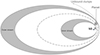 |
Fig. 1. Schematic illustration (not to scale) of the partial disruption of a planet around a NS. The dashed ellipse represents the orbit of the planet. The gray areas represent possible ranges of the clumps’ orbit in the inner and outer bound stream. The dotted ellipses at the fringe of these gray areas represent the orbits of the clumps generated near θ = θc. The solid ellipse in the inner stream represents the clumps produced near θ = 0, while the solid ellipse in the outer stream represents the clumps produced at somewhere between θ = 0 and θ = θc, depending on the structure of the planet. The curved arrow represents unbound clumps. |
When the planet passes through the pericenter, a number of clumps will be generated during the partial disruption process. The host NS, the surviving main part of the planet, and the clumps form a many-body system. Ignoring the interactions between the clumps, it can be simplified as a triple system composed of the NS, the remnant planet, and a particular clump. In this case, the gravitational perturbation from the planet plays an important role in the evolution of the clump’s orbit, which could lose its angular momentum due to the perturbation and fall toward the NS (Kurban et al. 2023). The Alfvén wave drag caused by the magnetic field of the NS can further facilitate the in-falling process (e.g.,Geng et al. 2020). The interaction between the major clumps and the NS will finally produce a series of X-ray bursts. We estimate the burst energy, duration, periodicity, and activity window in Sect. 3.
2.2. Key parameters
In our framework, we considered a rocky planet that is a pure Fe object, a pure MgSiO3 object, or a two-layer planet with an Fe core and an MgSiO3 mantle. The internal structure of such planets can be determined by using the equations of state (EOSs) that are widely used in exoplanet modeling (see Smith et al. 2018 for the EOS of Fe materials and Seager et al. 2007 for that of MgSiO3 materials). Table 1 lists some typical parameters of the three kinds of planets (see Kurban et al. 2023 for more details).
Typical parameters of the planets considered in our study and the timing parameters of the clumps originated from the inner side of the planet.
When the size of a planet is larger than 1000 km, self-gravity will dominate over the internal tensile stresses (Brown et al. 2017). The tidal disruption radius of such a self-gravity-dominated planet is rtd = Rpl(2M⋆/mpl)1/3. However, the degree of disruption depends on the impact parameter (β = rtd/rp) as well as the planet’s structure. A slight decrease in the pericenter may result in a complete disruption, while a small increase will lead to no mass loss at all (e.g., Guillochon & Ramirez-Ruiz 2013). To be more specific, a planet would be completely destroyed only when the tidal force from the NS exceeds the maximum self-gravitational force inside the planet but not the surface gravitational field. This means that the dense planet core is most difficult to destroy and could survive for slightly larger values of β (e.g., Coughlin & Nixon 2022a; Bandopadhyay et al. 2024). In short, a higher central density of the planet makes a complete disruption less likely. As a result, partial disruption could occur in a considerable range of β for a planet. In fact, numerical simulations (Guillochon et al. 2011; Guillochon & Ramirez-Ruiz 2013; Liu et al. 2013; Nixon et al. 2021) and analytic derivations (Coughlin & Nixon 2022a) show that a partial disruption occurs when rp ≈ 2rtd (β ≈ 0.5). In this study, we took this distance as a typical condition that the planet would be partially disrupted near the periastron (Kurban et al. 2022, 2023).
Taking rp ∼ 1011 cm, the eccentricity is e ∼ 0.992 for a planet with an orbital period of Porb = 240 days (a = 0.85 au), while it is e ∼ 0.994 for Porb = 400 days (a = 1.19 au). One may obtain a slightly wider parameter range when the diversity of the planet structure is considered (Kurban et al. 2022, 2023). Such a highly eccentric orbit satisfying rp ≈ 2rtd can be formed in the dynamical processes mentioned earlier. A simulation by Goulinski & Ribak (2018) showed that more than 99.1% of the captured planets form orbits with 0.85 < e ≲ 1 and a ∼ 1–104 au. The planet-planet scattering (e.g., Carrera et al. 2019) and the capture of a planet from a nearby planetary system via the Hills mechanism (e.g., Cufari et al. 2022) are the other two efficient ways to form highly eccentric orbits. In addition, an extremely high eccentricity can also be reached due to the Kozai-Lidov mechanism for a wide range of semimajor axis (e.g., Naoz 2016).
The clumps generated during the disruption will have slightly different orbits (see Fig. 1), which are determined by the planet’s binding energy and pericenter distance (Norman et al. 2021). For example, the clumps originating from the inner side of the planet will have a relatively small orbit. The semimajor axis of their orbits can be expressed as (Malamud & Perets 2020b; Brouwers et al. 2022)
where a is the planet’s original semimajor axis, d is the distance between the NS and the planet at the moment of the breakup (here d = rp), R is the displacement of the clump relative to the planet’s mass center at the moment of breakup (R = 0 corresponds to the center of the planet). Because the planet is in a bound orbit, the clumps in the inner stream are generally bound to the NS so that they can be relevant to the X-ray bursts studied in the work.
For clumps in the outer orbit stream, their semimajor axes can be calculated as  . From this relation, a critical displacement can be derived as Rcrit = d2/(2a − d). A clump is still bound to the NS if its displacement is R < Rcrit, while it is unbound for R > Rcrit (Malamud & Perets 2020b). Rcrit depends on the pericenter and binding energy of the planet. Combining the partial disruption condition of d = rp = 2rtd, we can assess the boundness of the clumps in the outer stream. It is found that unbound (free) clumps could be generated in the following cases considered here: an Fe planet with mpl = 18.1 M⊕ in the case of Porb = 238 days; an Fe planet with mpl = 10.1, 18.1 M⊕, an MgSO3 planet with mpl = 18.2 M⊕, and a two-layer planet with mpl = 12.8 M⊕ for the case Porb = 398 days. The outer stream clumps generated from other planets considered in our study are all bound to the NS. The orbits of these bound clumps will also be affected by the remnant planet’s gravity and can be altered significantly due to the scattering effect. They may even be ejected from the system finally. As a result, the clumps in the outer stream are less likely to collide with the NS (especially on short timescales), and their involvement in the generation of X-ray bursts is not expected.
In the case of a full disruption, the material in a bound orbit returns to the periastron on a timescale of  (Lacy et al. 1982; Norman et al. 2021). We note that this expression underestimates the return time if rtd is replaced by rp for deep encounters (Rossi et al. 2021; Coughlin & Nixon 2022a). For the partial disruption in our framework, the clump’s return time approximately equals its orbital period,
 ![$ t_{\mathrm{ret}} \approx P_{\mathrm{orb}}^{\mathrm{cl}} = \sqrt{4 \pi^2 a_{\mathrm{cl}}^3/[G (M_{\star} + m_{\mathrm{cl}})]} $](/articles/aa/full_html/2024/06/aa47828-23/aa47828-23-eq12.gif) . The clump’s orbit should satisfy rp = acl(1 − ecl)±R (here “+” and “−” for the clumps in the inner and outer stream, respectively), from which one can derive the eccentricity as ecl = 1 − (rp ∓ R)/acl. Since the clumps are stripped off from the surface of the planet, we took R ∼ Rpl when calculating their orbital parameters.
. The clump’s orbit should satisfy rp = acl(1 − ecl)±R (here “+” and “−” for the clumps in the inner and outer stream, respectively), from which one can derive the eccentricity as ecl = 1 − (rp ∓ R)/acl. Since the clumps are stripped off from the surface of the planet, we took R ∼ Rpl when calculating their orbital parameters.
After the partial disruption, clumps of different sizes may be generated. Larger homogeneous monolithic clumps generally have larger cohesive strength (e.g., Malamud & Perets 2020b). Smaller ones may merge to form larger clumps due to gravitational instabilities in the hydrodynamical evolution of the debris disk (Coughlin & Nixon 2015), which itself depends on the EOS and is preferred for EOSs stiffer than γ = 5/3 (Coughlin et al. 2016a,b, 2020; Coughlin 2023; Fancher et al. 2023). In our cases, the characteristics of the massive clumps formed through the accumulation of debris due to gravitational instabilities are similar to that of the rubble pile asteroids, which have a material strength in the range of ∼1 Pa–1000 Pa (Walsh 2018).
Veras et al. (2014) have investigated the tidal disruption of rubble pile asteroids by assuming that the asteroid is frictionless, which means they essentially ignored the cohesive strength. The classical Roche approximation based solely on self-gravity could be applied in that case. However, they have also pointed out that cohesive strength could play a role in the process. Especially, the breakup distance of small bodies (< 1000 km) is mainly determined by the material strength (Brown et al. 2017). The larger the cohesive strength is, the closer it gets to the central star (Brouwers et al. 2022). The homogeneous monolithic clumps and the rubble pile clumps formed in our cases have different material strengths so that they break up at different distances that are smaller than the partial disruption radius of the planet. In short, the clumps can remain intact even when they are much closer to the NS due to their cohesive strength. For them, the breakup distance is (Zhang et al. 2021b)
where rcl and ρcl are the radius (here we assumed that the clump is spherical for the sake of simplicity) and density of the clump, respectively; k is a function of the internal friction angle, ϕ, and the cohesive strength, C:  . The friction angle of geological materials commonly ranges from 25° to 50° (e.g., Holsapple & Michel 2008; Bareither et al. 2008; Jiang et al. 2018; Villeneuve & Heap 2021). The typical strength is C ∼ 1 Pa for comets (Gundlach & Blum 2016) and C ∼ 1 Pa–1000 Pa for rubble pile asteroids (Walsh 2018), while it is in the range 0.1 Mpa–50 MPa for monolithic asteroids/meteorites (Schöpfer et al. 2009; Ostrowski & Bryson 2019; Pohl & Britt 2020; Veras & Scheeres 2020; Villeneuve & Heap 2021). As a result, the breakup distance for the clumps considered here is ∼109–1010 cm.
3. X-ray bursts
3.1. Periodicity and activity window
The periodicity and active window of X-ray bursts are determined by the orbital evolution of the clumps generated in the NS planet system. It can be simplified as a triple system composed of the NS, the remnant planet, and a particular clump. The clump’s orbit evolves under the influence of strong gravitational perturbation from the remnant planet.
In a triple system where a test particle revolves around its host in a close inner orbit while a third object moves around in an outer orbit, the eccentricity of the test particle can be significantly altered by the outer object. This is known as the Kozai-Lidov mechanism, which can explain the long-term orbital evolution of triple systems in the hierarchical limit (Kozai 1962; Lidov 1962). In recent decades, it has been further developed and applied to various mildly hierarchical or non-hierarchical systems. The hierarchy of a system is mainly measured by a parameter defined as ![$ \epsilon = a_{1} e_{2}/[a_{2}(1 - e_{2}^2)] $](/articles/aa/full_html/2024/06/aa47828-23/aa47828-23-eq15.gif) , which actually is the coefficient of the octupole-order interaction term (Lithwick & Naoz 2011; Li et al. 2014). Here the eccentricity (e) and semimajor axis (a) of the inner and outer orbits are denoted by subscripts 1 and 2, respectively. ϵ parameterizes the size of the external orbit versus that of the internal orbit. The initial orbital parameters of a triple system have an obvious influence on its final fate after a long-term dynamic evolution. A system with ϵ ≤ 0.1 is hierarchical and stable, a system with ϵ > 0.3 is nonhierarchical and unstable, while 0.1 < ϵ ≤ 0.3 corresponds to the mildly hierarchical condition (Naoz 2016). We note that the Kozai-Lidov mechanism (secular interaction) is broken down for the nonhierarchical and unstable systems so that it cannot provide a meaningful description for the orbital evolution at all (Perets & Kratter 2012; Katz & Dong 2012). Strong perturbations from the outer orbit object (Toonen et al. 2022) lead the test particle to effectively lose its angular momentum on a timescale on the order of the inner orbit period, causing it to collide with the central object (e.g., Antonini et al. 2014, 2016; He & Petrovich 2018; Hamers et al. 2022).
, which actually is the coefficient of the octupole-order interaction term (Lithwick & Naoz 2011; Li et al. 2014). Here the eccentricity (e) and semimajor axis (a) of the inner and outer orbits are denoted by subscripts 1 and 2, respectively. ϵ parameterizes the size of the external orbit versus that of the internal orbit. The initial orbital parameters of a triple system have an obvious influence on its final fate after a long-term dynamic evolution. A system with ϵ ≤ 0.1 is hierarchical and stable, a system with ϵ > 0.3 is nonhierarchical and unstable, while 0.1 < ϵ ≤ 0.3 corresponds to the mildly hierarchical condition (Naoz 2016). We note that the Kozai-Lidov mechanism (secular interaction) is broken down for the nonhierarchical and unstable systems so that it cannot provide a meaningful description for the orbital evolution at all (Perets & Kratter 2012; Katz & Dong 2012). Strong perturbations from the outer orbit object (Toonen et al. 2022) lead the test particle to effectively lose its angular momentum on a timescale on the order of the inner orbit period, causing it to collide with the central object (e.g., Antonini et al. 2014, 2016; He & Petrovich 2018; Hamers et al. 2022).
In our framework, the parameters of the clumps in the inner stream satisfy ϵ > 0.3, which means that they are in a nonhierarchical and unstable regime. The secular approximation (Kozai-Lidov mechanism) is broken down for them. The surviving major portion of the planet plays the role of the outer object, which can significantly alter the clump’s orbit and cause it to fall onto the NS on a timescale comparable to a few orbital periods (Kurban et al. 2023). In fact, in a recent study, it was shown that energy exchange between the clump and the remnant planet could occur due to strong gravitational interactions, which leads the clump’s periastron distance (rp) to abruptly change to a very small value (e.g., Zhang et al. 2023). Below, we present a rough estimate for the travel time that a clump experiences from its birth to the final collision with the NS. The total duration for most clumps to collide with the NS (i.e., the active window) can also be estimated.
After the partial disruption, a clump originating from the inner side of the planet will move in an inner orbit. The travel time for it to fall onto the NS depends on its return time (tret) to the periastron as well as the evolution timescale of its angular momentum (tevo). The return time approximately equals its orbital period,  . After the formation of the inner orbit, the clump loses its angular momentum (
 ) on a timescale of tevo due to gravitational perturbations. This is expected to occur when the clump passes through the periastron at the end of the second or third orbit because tevo is much less than
  under the condition of mpl > 2M⊕ and Porb > 100 days (Kurban et al. 2023). Therefore, the clump’s travel time from its birth at the planet to its collision with the NS can be approximated as (Kurban et al. 2023)
where tevo is expressed as (e.g., Antonini et al. 2014)
![$$ \begin{aligned} t_{\rm evo} = \left(\frac{1}{j_{\rm cl}}\frac{\mathrm{d}j_{\rm cl}}{\mathrm{d}t}\right)^{-1} \approx P_{\rm orb}^\mathrm{cl}\frac{1}{5\pi } \frac{M_{\star }}{m_{\rm pl}} \left[ \frac{a(1 - e)}{a_{\rm cl}} \right]^3 \sqrt{1 - e_{\rm cl}}. \end{aligned} $$](/articles/aa/full_html/2024/06/aa47828-23/aa47828-23-eq20.gif)
We note that different clumps with slightly different orbital periods will arrive at the NS at different times.
Figure 2 shows the travel time of a clump in the innermost orbit for pure Fe planets, MgSiO3 planets, and two-layer planets. From this figure, we see that the clumps will fall onto the NS on a short timescale on the order of its own orbital period, which is affected by the orbit and composition of the planet.
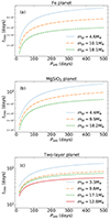 |
Fig. 2. Travel time (ttrav) of the clumps in the innermost orbit as a function of the planet’s orbital period (Porb). Three kinds of planets are considered: (a) Fe planets, (b) MgSiO3 planets, and (c) two-layer planets. The mass of the planet (mpl) is marked in each panel. |
The activity widow of the bursts can be estimated by considering the dispersion of the arrival time of various clumps with slightly different orbital periods. We can consider the case of two clumps: one has an orbital period of  , the other has a different orbital period of
  , where
  is their difference in orbit. Their difference in arrival time can be calculated from the derivative of travel time as
  , which is just the time interval between two successive collisions.
The simulations by Malamud & Perets (2020b,a) show that the distribution of the orbital period of inner bound clumps can range from  to Porb in a full disruption. However, the competition between the tidal force and the self-gravity continuously evolves over the encounter. The largest partial disruption distance for a planet is ∼2.7rtd (Guillochon et al. 2011; Liu et al. 2013). During a strong encounter, the mass loss from the planet continues till a separation of several times rtd (e.g., Ryu et al. 2020). For the partial disruption cases discussed here, the mass loss will continue until the planet’s separation from the NS is rc ∼ 4rtd. In other words, the mass loss occurs until the phase θ ∼ θc, where θc is the true anomaly at r = rc. When θ > θc (or r > rc), new clumps could not be generated till the next periastron passage. For the inner and outer bound streams, the clumps marginally bound to the remnant planet will be re-accreted by the surviving core of the planet after a few dynamical timescales defined by
  (e.g., Guillochon et al. 2011; Coughlin & Nixon 2019). We note that the dynamical timescale is typically tdyn ∼ 6–14 min, which depends on the structure of the planets. On the other hand, the clumps that are not bound to the remnant planet will return to the periastron and continue to orbit around the NS (e.g., Guillochon et al. 2011). One can obtain the critical semimajor axis acl, c (or the critical orbital period
  ) using the critical separation of d = rc ∼ 4rtd. Thus, for the clumps in the inner orbits, we expect their orbital periods to be between
  and
and  . The upper limit of
  would then be
  . We used this parameter to estimate Δttrav, up, which is just the activity window of X-ray bursts in our framework.
Figure 3 illustrates Δttrav as a function of  for planets with different orbital period and composition. We note that
  satisfies
  , which determines the range of the active window for the X-ray bursts. Δttrav, up is sensitive to both rp and rc. A too-small rp may cause the period to completely disappear.
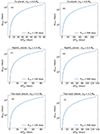 |
Fig. 3. Difference in the travel time (Δttrav) as a function of the clump’s orbital period difference ( |


Table 1 lists the timing parameters of the clumps disrupted from various planets with different compositions, masses, and orbital periods.  and
and  are the orbital periods of the clumps in the innermost orbit and the clumps stripped off from the planet at θc (or r = rc), respectively. ttrav and ttrav, c are their travel times, and
  and Δttrav, up are their orbital period difference and travel time difference, respectively. It can be seen from this table that these parameters are affected by the structure and orbital period of the planet. Generally, a larger Porb leads to a larger Δttrav, up. For planets with a particular Porb, the structure is also an important factor: Δttrav, up decreases with the increase in compactness (mpl/Rpl).
3.2. Energy and duration
In the last section we investigated the properties of clumps and show that the clumps fall onto the NS on a short timescale. The collision of a small body (asteroid) with a NS can produce X-ray bursts (Huang & Geng 2014; Geng et al. 2020; Dai et al. 2016; Dai 2020). The gravitational potential energy of the small body will transform to X-ray burst energy as (e.g., Geng et al. 2020; Dai 2020)
where η (η < 1) is the energy transforming efficiency.
In our case, the range of the mass of the clumps can be relatively wide. For example, simulations show that the size of clumps generated during the partial disruption ranges from a few kilometers to ∼100 km (Malamud & Perets 2020a,b). It depends on the distance to the NS as well as its intrinsic material strength. On the other hand, if a clump is too large, it cannot resist the tidal force and will further break up during its falling toward the NS. The clumps will interact with the magnetosphere and produce Alfvén wings at the light cylinder radius, RLC = cPspin/2π (Cordes & Shannon 2008; Mottez & Heyvaerts 2011; Mottez et al. 2013a,b; Chen & Hu 2022), which further helps the NS capture the clumps (Geng et al. 2020) at the Alfvén radius. The Alfvén radius is determined by assuming that the kinetic energy equals the magnetic energy, namely  , where
  and BRA = B⋆(R⋆/RA)3 are the free-fall velocity and magnetic field strength at the distance RA from the NS, respectively. The Alfvén radius RA then can be calculated as
  . Taking R⋆ = 10 km and ρcl = 5–8 g cm−3 (the surface density of the planet with different compositions), we get RA = (4.43 − 4.04)×107 cm for SGR 1935+2154 and RA = (1.83 − 1.67)×107 cm for SGR 1806-20.
Depending on the size and mass of the clumps near RLC, X-ray bursts with different energies can be produced. Following Eq. (2), we can calculate the upper limit of the clump size at the light cylinder. Figure 4 shows the breakup distance as a function of the clump mass. The dotted, dashed, and dash-dotted lines correspond to MgSO3 clumps (ρcl = 5 g cm−3) with cohesive strengths of C = 1 kPa, 1 MPa, and 10 MPa, respectively. These C values are typical for rocky materials (Gundlach & Blum 2016; Pohl & Britt 2020; Veras & Scheeres 2020; Villeneuve & Heap 2021). Here, an internal friction angle of ϕ = 45° is used for rocky materials (e.g., Holsapple & Michel 2008; Bareither et al. 2008; Villeneuve & Heap 2021). The solid line represents iron clumps (ρcl = 8 g cm−3), for which C = 50 MPa (Ostrowski & Bryson 2019; Pohl & Britt 2020) and ϕ = 37° (Jiang et al. 2018) are adopted. The horizontal lines represent the light cylinder radius (RLC) of NS with a spin period of 11.79 s (1E 1841-045, Dib & Kaspi (2014)), 7.55 s (SGR 1806-20), and 3.245 s (SGR 1935+2154), respectively. From Fig. 4, we see that the mass range of the clumps that safely enter RLC is up to ∼1022 g, which satisfies the energy budget of X-ray bursts. We notice that RLC ∼ 1010 cm is much larger than RA. But this is not a problem in our case, since the clump can effectively lose its angular momentum due to perturbation when it is still far from the light cylinder.
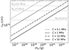 |
Fig. 4. Breakup distance as a function of the clump mass. The clump is a rocky (MgSO3) object with a density of ρcl = 5 g cm−3 and an internal friction angle of ϕ = 45°. The dotted, dashed, and dash-dotted line corresponds to the cohesive strength of C= 0.1, 1, and 10 MPa, respectively. The solid line represents an iron clump with ρcl = 8 g cm−3, C = 50 MPa, and ϕ = 37°. The horizontal lines represent the light cylinder radii for NSs with different spin periods. |
The energies of the X-ray bursts produced through the interactions between the clumps and the NS can be calculated from Eq. (5). The results are plotted in panel a of Fig. 5. It shows that the energetics can be up to ∼1043 erg, which is large enough to account for the energies of the short X-ray bursts observed from SGR 1935+2154 and SGR 1806-20.
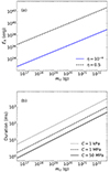 |
Fig. 5. Energy (panel a) and duration (panel b) of X-ray bursts as a function of the clump mass. In panel a the dashed and solid lines correspond to an energy transforming efficiency of η = 0.5 and η = 10−4, respectively. In panel b the dotted and dashed lines represent the MgSO3 clumps with a cohesive strength of C = 1 kPa and C = 1 MPa, respectively. The solid line corresponds to iron clumps with C = 50 MPa. |
The burst duration can be calculated as (e.g., Dai 2020)
where rstr is the breakup distance of the clumps given by Eq. (2). Here, a relation of rcl = (3mcl/4πρcl)1/3 is adopted. According to Eq. (6), the burst duration can range from a few milliseconds to seconds, as shown in panel b of Fig. 5. We see that the burst duration is also compatible with the observations.
4. Comparison with observations
The model described in Sect. 3 can explain the periodical X-ray bursts observed from SGRs. Here we confront the theoretical burst energy, duration, period, and activity window with the observations.
4.1. SGR 1935+2154
Figure 6 illustrates the burst energy as a function of duration for SGR 1935+2154. The observational data points of SGR 1935+2154 are shown by assuming a distance of 9 kpc for the source (Lin et al. 2020a,b; Cai et al. 2022a,b). The solid lines are calculated for different C and η values. We see that the energy budgets can be easily satisfied when the two parameters are evaluated in reasonable ranges.
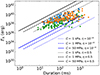 |
Fig. 6. X-ray bursts from SGR 1935+2154 plotted on the energy-duration plane. The orange (Lin et al. 2020a), blue (Lin et al. 2020b), and green (Cai et al. 2022b,a) dots represent the bursts observed by various groups. The lines of different styles are the theoretical results calculated by taking different values for the cohesive strength (C) and energy transforming efficiency (η). |
The periodicity and activity window of the X-ray bursts from SGR 1935+2154 can also be explained. From Fig. 3, we see that when we take the orbit period as Porb = 238 days and the upper limit of the period difference as  days, then the arrival time difference is Δttrav = 150 days. This agrees well with the observed ∼150 day activity window of the SGR.
4.2. SGR 1806-20
More than 3000 X-ray bursts from SGR 1806-20 have been detected (see Göǧüş et al. 2000; Prieskorn & Kaaret 2012; Kırmızıbayrak et al. 2017 and references therein). Detailed spectroscopic analyses were performed on some bursts (Atteia et al. 1987; Kouveliotou et al. 1987; Fenimore et al. 1994; Kırmızıbayrak et al. 2017). The observation data of the Rossi X-ray Timing Explorer (RXTE) show that the observed fluence ranges between ∼10−10 and 10−7 erg cm−2 (Kırmızıbayrak et al. 2017). Similarly, the fluence of the X-ray bursts detected by the International Cometary Explorer (ICE) is in the range ∼10−8–10−5 erg cm−2 (Atteia et al. 1987; Kouveliotou et al. 1987; Fenimore et al. 1994; Göǧüş et al. 2000). We notice that the fluence of the ICE bursts is higher than that of the RXTE bursts by about two orders of magnitude. This may be due to the fact that ICE has a much higher sensitivity, meaning that weaker bursts can be recorded.
Figure 7 plots the burst energy as a function of the duration. The isotropic energy of each burst is calculated by taking the distance as 8.7 kpc (Bibby et al. 2008). The data points correspond to the bursts observed by RXTE, whose energy ranges between ∼1037 and 1039 erg. The shaded area illustrates the energy range of the X-ray bursts detected by ICE. We see that the energetics of the observed X-ray bursts can be explained well by our model.
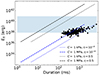 |
Fig. 7. X-ray bursts from SGR 1806-20 plotted on the energy-duration plane. The black dots denote the observational data (Kırmızıbayrak et al. 2017). The lines are the theoretical results calculated by taking different values for the cohesive strength (C) and energy transforming efficiency (η). The shaded area represents the energy range of the bursts detected by the ICE detector (Göǧüş et al. 2000). |
Most of the X-ray bursts from SGR 1806-20 are concentrated near the phase of ∼0.58 (Zhang et al. 2021a). However, the bursts could also appear at all the period phases. In other words, the periodicity of SGR 1806-20 is not as strict as that of SGR 1935+2154. The reason for such a relatively poor periodicity may be that the system has a small rp, which can effectively smear the periodicity to some extent (see Sect. 3).
5. Conclusions and discussion
In this study, the periodicity and other properties of repeating X-ray bursts from two magnetars are explained by the interaction between a NS and its close-in planet. In our model, a rocky planet moves around a NS in a highly eccentric orbit. The planet is partially disrupted every time it passes through the periastron of the orbit due to the tidal force of its compact host. During the process, clumps ranging from a few kilometers to ∼100 km are produced. The clumps can lose their angular momentum under the influence of the remnant planet and fall toward the NS. They are further disrupted and captured by the strong magnetic field when they enter the magnetosphere of the magnetar and/or NS. The interaction between the NS and the clumps produces a series of X-ray bursts. We show that the mass of the clumps that can enter the light cylinder radius is up to ∼1022 g, which is mainly determined by the clump’s shearing strength. The energy of the X-ray bursts produced in this way can be as high as ∼1043 erg, and their durations typically range from a few milliseconds to seconds. All these features are consistent with observations. The bursts will show a clear periodicity due to the orbital motion of the planet. The active window of the two SGRs can also be explained (Zhang et al. 2021a; Zou et al. 2021; Xie et al. 2022).
It was reported that there were no bursts during some of the periods (Zhang et al. 2021a; Zou et al. 2021). In our framework, this can be caused by two factors. First, the asymmetry of mass loss can alter the orbit. In the planet’s subsequent passage through the periastron, the mass loss would not occur if rp were larger than the maximum partial disruption distance (rtd, max). As a result, one would not be able to observe any bursts from the system. Second, the Kozai-Lidov effect may be very complicated if the system contains more than one planet. Multi-planet systems have been identified in a few cases, such as PSR 1257+12 (Wolszczan & Frail 1992), PSR B0943+10 (Suleymanova & Rodin 2014), and PSR J1807-2459 (Ransom et al. 2001; Ray & Loeb 2017). If the parameters of such systems satisfy some special conditions, rapid eccentricity oscillation may occur due to the Kozai-Lidov effect, causing complicated variations in the periastron distance (rp). There would be no mass loss if rp > rtd, max during the oscillation process, and thus no bursts would occur.
There is no clear correlation between the burst energy and waiting time for the X-ray bursts from SGR 1806-20 (Göǧüş et al. 2000). This is consistent with the expectation of self-organized criticality (Katz 1986; Bak et al. 1987). In our model, the waiting time is simply the interval time between two successive collisions, which depends on the spatial distribution of in-falling clumps. The breakup distance of the clumps is generally determined by their composition, but the breakup procedure itself is a random process that leads to a stochastic distribution of the size and in-fall time for the sub-clumps. As a result, there is no correlation between the burst energy and the waiting time in our framework, which agrees well with the observations of SGR 1806-20.
For SGR 1806-20, a giant flare, whose total energy release was 4.01 × 1046 erg, was observed on 27 December 2004 (Hurley et al. 2005). Such an energetic flare is a rare event and one that had only been observed from this source once before. If it were due to a collision event, then the clump mass would be several times 1026 g. In the partial tidal disruption process considered here, the generation of such a massive clump is possible (e.g., Malamud & Perets 2020a,b). Considering the collisions between clumps, the possibility of some large objects being scattered toward the host star exists, but the probability is low and it should be a rare event (e.g., Cordes & Shannon 2008). If the clump is composed of materials with a high cohesive strength, it can retain a high mass before arriving at the light cylinder and will eventually collide with the NS and/or SS to produce a giant flare (e.g., Zhang et al. 2000; Usov 2001). Therefore, giant flares are rare events in our framework, but they could reoccur in the future.
It is interesting to note that periodic X-ray flares are observed from Jupiter (Yao et al. 2021), which may be evidence that X-ray bursts can be generated via the interaction of external materials with a planet in the Solar System. It was argued that the charged ions that originate from the gas spewed into space due to giant volcano events on Jupiter’s moon (Io) could flow onto Jupiter along magnetic field lines, leading to an energy release in the form of X-rays (Cowley & Bunce 2001; Yao et al. 2021). Such phenomena could be universal and present across many different environments in space (Dunn et al. 2017; Yao et al. 2021; Mori et al. 2022). The X-ray bursts generated through the interaction of a NS with clumps disrupted from a planet are to some extent similar phenomena.
Finally, we would like to mention that the dynamics of the clumps and the evolution of their angular momentum is highly complicated. Even in the asteroid-disruption explanation for the white dwarf pollution, it is still unclear how disrupted asteroids ultimately lose enough angular momentum to fall onto the white dwarf. There is a similar issue for the partial TDEs. Self-intersection shocks arising from stream–stream collisions, which themselves arise from relativistic apsidal precession, might play a role in the dissipation. But this could be inefficient in some circumstances. In our cases of partial disruption, the remnant planet may act as a third object responsible for dissipation. Nevertheless, it is still possible that in some cases the clumps may simply orbit around the NS many times, instead of producing prompt accretion and X-ray bursts.
Acknowledgments
We would like to thank the anonymous referee for helpful suggestions that led to significant improvement of our study. This work was Sponsored by the Natural Science Foundation of Xinjiang Uygur Autonomous Region (No. 2022D01A363), the National Natural Science Foundation of China (Grant Nos. 12033001, 12288102, 12273028 12041304, 12233002, 12041306), the Natural Science Foundation of Xinjiang Uygur Autonomous Region (No. 2023D01E20), the Major Science and Technology Program of Xinjiang Uygur Autonomous Region (Nos. 2022A03013-1, 2022A03013-3), National Key R&D Program of China (2021YFA0718500), National SKA Program of China No. 2020SKA0120300, the Tianshan Talents Training Program (2023TSYCTD0013). Y.F.H. acknowledges the support from the Xinjiang Tianchi Program. AK acknowledges the support from the Tianchi Talents Project of Xinjiang Uygur Autonomous Region and the special research assistance project of the Chinese Academy of Sciences (CAS). This work was also partially supported by the Operation, Maintenance and Upgrading Fund for Astronomical Telescopes and Facility Instruments, budgeted from the Ministry of Finance of China (MOF) and administrated by the CAS, the Urumqi Nanshan Astronomy and Deep Space Exploration Observation and Research Station of Xinjiang (XJYWZ2303).
References
- Antonini, F., Murray, N., & Mikkola, S. 2014, ApJ, 781, 45 [NASA ADS] [CrossRef] [Google Scholar]
- Antonini, F., Chatterjee, S., Rodriguez, C. L., et al. 2016, ApJ, 816, 65 [NASA ADS] [CrossRef] [Google Scholar]
- Atteia, J. L., Boer, M., Hurley, K., et al. 1987, ApJ, 320, L105 [NASA ADS] [CrossRef] [Google Scholar]
- Auchettl, K., Guillochon, J., & Ramirez-Ruiz, E. 2017, ApJ, 838, 149 [Google Scholar]
- Bailes, M., Lyne, A. G., & Shemar, S. L. 1991, Nature, 352, 311 [NASA ADS] [CrossRef] [Google Scholar]
- Bak, P., Tang, C., & Wiesenfeld, K. 1987, Phys. Rev. Lett., 59, 381 [NASA ADS] [CrossRef] [Google Scholar]
- Bandopadhyay, A., Fancher, J., Athian, A., et al. 2024, ApJ, 961, L2 [NASA ADS] [CrossRef] [Google Scholar]
- Bareither, C. A., Edil, T. B., Benson, C. H., & Mickelson, D. M. 2008, J. Geotech. Geoenviron. Eng., 134, 1476 [CrossRef] [Google Scholar]
- Bhattacharya, D., & van den Heuvel, E. P. J. 1991, Phys. Rep., 203, 1 [Google Scholar]
- Bibby, J. L., Crowther, P. A., Furness, J. P., & Clark, J. S. 2008, MNRAS, 386, L23 [NASA ADS] [CrossRef] [Google Scholar]
- Bloom, J. S., Giannios, D., Metzger, B. D., et al. 2011, Science, 333, 203 [CrossRef] [PubMed] [Google Scholar]
- Brouwers, M. G., Bonsor, A., & Malamud, U. 2022, MNRAS, 509, 2404 [NASA ADS] [Google Scholar]
- Brown, J. C., Veras, D., & Gänsicke, B. T. 2017, MNRAS, 468, 1575 [NASA ADS] [CrossRef] [Google Scholar]
- Cai, C., Xiong, S.-L., Lin, L., et al. 2022a, ApJS, 260, 25 [NASA ADS] [CrossRef] [Google Scholar]
- Cai, C., Xue, W.-C., Li, C.-K., et al. 2022b, ApJS, 260, 24 [NASA ADS] [CrossRef] [Google Scholar]
- Campana, S., Lodato, G., D’Avanzo, P., et al. 2011, Nature, 480, 69 [NASA ADS] [CrossRef] [Google Scholar]
- Carrera, D., Raymond, S. N., & Davies, M. B. 2019, A&A, 629, L7 [NASA ADS] [CrossRef] [EDP Sciences] [Google Scholar]
- Cendes, Y., Berger, E., Alexander, K. D., et al. 2022, ApJ, 938, 28 [NASA ADS] [CrossRef] [Google Scholar]
- Cendes, Y., Berger, E., Alexander, K. D., et al. 2023, ApJ, submitted, [arXiv:2308.13595] [Google Scholar]
- Cenko, S. B., Krimm, H. A., Horesh, A., et al. 2012, ApJ, 753, 77 [NASA ADS] [CrossRef] [Google Scholar]
- Chatterjee, P., Hernquist, L., & Narayan, R. 2000, ApJ, 534, 373 [NASA ADS] [CrossRef] [Google Scholar]
- Chen, Y., & Hu, Q. 2022, ApJ, 924, 43 [NASA ADS] [CrossRef] [Google Scholar]
- Colgate, S. A., & Petschek, A. G. 1981, ApJ, 248, 771 [NASA ADS] [CrossRef] [Google Scholar]
- Cordes, J. M., & Shannon, R. M. 2008, ApJ, 682, 1152 [NASA ADS] [CrossRef] [Google Scholar]
- Coughlin, E. R. 2023, MNRAS, 522, 5500 [NASA ADS] [CrossRef] [Google Scholar]
- Coughlin, E. R., & Nixon, C. 2015, ApJ, 808, L11 [NASA ADS] [CrossRef] [Google Scholar]
- Coughlin, E. R., & Nixon, C. J. 2019, ApJ, 883, L17 [NASA ADS] [CrossRef] [Google Scholar]
- Coughlin, E. R., & Nixon, C. J. 2022a, MNRAS, 517, L26 [NASA ADS] [CrossRef] [Google Scholar]
- Coughlin, E. R., & Nixon, C. J. 2022b, ApJ, 926, 47 [CrossRef] [Google Scholar]
- Coughlin, E. R., Nixon, C., Begelman, M. C., & Armitage, P. J. 2016a, MNRAS, 459, 3089 [NASA ADS] [CrossRef] [Google Scholar]
- Coughlin, E. R., Nixon, C., Begelman, M. C., Armitage, P. J., & Price, D. J. 2016b, MNRAS, 455, 3612 [CrossRef] [Google Scholar]
- Coughlin, E. R., Nixon, C. J., & Miles, P. R. 2020, ApJ, 900, L39 [NASA ADS] [CrossRef] [Google Scholar]
- Cowley, S. W. H., & Bunce, E. J. 2001, Planet. Space Sci., 49, 1067 [NASA ADS] [CrossRef] [Google Scholar]
- Cufari, M., Coughlin, E. R., & Nixon, C. J. 2022, ApJ, 929, L20 [NASA ADS] [CrossRef] [Google Scholar]
- Currie, T., & Hansen, B. 2007, ApJ, 666, 1232 [CrossRef] [Google Scholar]
- Dai, Z. G. 2020, ApJ, 897, L40 [NASA ADS] [CrossRef] [Google Scholar]
- Dai, Z. G., Wang, J. S., Wu, X. F., & Huang, Y. F. 2016, ApJ, 829, 27 [NASA ADS] [CrossRef] [Google Scholar]
- Dib, R., & Kaspi, V. M. 2014, ApJ, 784, 37 [NASA ADS] [CrossRef] [Google Scholar]
- Dunn, W. R., Branduardi-Raymont, G., Ray, L. C., et al. 2017, Nat. Astron., 1, 758 [NASA ADS] [CrossRef] [Google Scholar]
- Evans, P. A., Nixon, C. J., Campana, S., et al. 2023, Nat. Astron., 7, 1368 [NASA ADS] [CrossRef] [Google Scholar]
- Fancher, J., Coughlin, E. R., & Nixon, C. J. 2023, MNRAS, 526, 2323 [NASA ADS] [CrossRef] [Google Scholar]
- Fenimore, E. E., Laros, J. G., & Ulmer, A. 1994, ApJ, 432, 742 [NASA ADS] [CrossRef] [Google Scholar]
- Geng, J. J., & Huang, Y. F. 2015, ApJ, 809, 24 [NASA ADS] [CrossRef] [Google Scholar]
- Geng, J.-J., Li, B., Li, L.-B., et al. 2020, ApJ, 898, L55 [NASA ADS] [CrossRef] [Google Scholar]
- Geng, J., Li, B., & Huang, Y. 2021, The Innovation, 2, 100152 [NASA ADS] [CrossRef] [Google Scholar]
- Gezari, S. 2021, ARA&A, 59, 21 [NASA ADS] [CrossRef] [Google Scholar]
- Gill, R., & Heyl, J. S. 2010, MNRAS, 407, 1926 [NASA ADS] [CrossRef] [Google Scholar]
- Göǧüş, E., Woods, P. M., Kouveliotou, C., et al. 2000, ApJ, 532, L121 [CrossRef] [Google Scholar]
- Goulinski, N., & Ribak, E. N. 2018, MNRAS, 473, 1589 [NASA ADS] [Google Scholar]
- Gourgouliatos, K. N., & Esposito, P. 2018, in The Physics and Astrophysics of Neutron Stars, eds. L. Rezzolla, P. Pizzochero, D. I. Jones, N. Rea, & I. Vidaña (Cham: Springer International Publishing), Astrophys. Space Sci. Lib., 457, 57 [NASA ADS] [CrossRef] [Google Scholar]
- Guillochon, J., & Ramirez-Ruiz, E. 2013, ApJ, 767, 25 [NASA ADS] [CrossRef] [Google Scholar]
- Guillochon, J., Ramirez-Ruiz, E., & Lin, D. 2011, ApJ, 732, 74 [NASA ADS] [CrossRef] [Google Scholar]
- Guillochon, J., Manukian, H., & Ramirez-Ruiz, E. 2014, ApJ, 783, 23 [NASA ADS] [CrossRef] [Google Scholar]
- Gundlach, B., & Blum, J. 2016, A&A, 589, A111 [NASA ADS] [CrossRef] [EDP Sciences] [Google Scholar]
- Hamers, A. S., Perets, H. B., Thompson, T. A., & Neunteufel, P. 2022, ApJ, 925, 178 [NASA ADS] [CrossRef] [Google Scholar]
- Hansen, B. M. S., Shih, H.-Y., & Currie, T. 2009, ApJ, 691, 382 [NASA ADS] [CrossRef] [Google Scholar]
- He, M. Y., & Petrovich, C. 2018, MNRAS, 474, 20 [NASA ADS] [CrossRef] [Google Scholar]
- Hills, J. G. 1975, Nature, 254, 295 [Google Scholar]
- Holsapple, K. A., & Michel, P. 2008, Icarus, 193, 283 [NASA ADS] [CrossRef] [Google Scholar]
- Hong, Y.-C., Raymond, S. N., Nicholson, P. D., & Lunine, J. I. 2018, ApJ, 852, 85 [NASA ADS] [CrossRef] [Google Scholar]
- Huang, Y. F., & Geng, J. J. 2014, ApJ, 782, L20 [NASA ADS] [CrossRef] [Google Scholar]
- Huang, Y. F., & Yu, Y. B. 2017, ApJ, 848, 115 [NASA ADS] [CrossRef] [Google Scholar]
- Huang, S., Jiang, N., Shen, R.-F., Wang, T., & Sheng, Z. 2023, ApJ, 956, L46 [NASA ADS] [CrossRef] [Google Scholar]
- Hurley, K., Boggs, S. E., Smith, D. M., et al. 2005, Nature, 434, 1098 [NASA ADS] [CrossRef] [Google Scholar]
- Israel, G. L., Esposito, P., Rea, N., et al. 2016, MNRAS, 457, 3448 [NASA ADS] [CrossRef] [Google Scholar]
- Jiang, P., Qiu, L., Li, N., et al. 2018, Adv. Civil Eng., 2018, 8 [Google Scholar]
- Kaspi, V. M., & Beloborodov, A. M. 2017, ARA&A, 55, 261 [Google Scholar]
- Katz, J. I. 1986, J. Geophys. Res., 91, 10,412 [Google Scholar]
- Katz, J. I. 1996, ApJ, 463, 305 [NASA ADS] [CrossRef] [Google Scholar]
- Katz, B., & Dong, S. 2012, arXiv e-prints [arXiv:1211.4584] [Google Scholar]
- Kırmızıbayrak, D., Şaşmaz Muş, S., Kaneko, Y., & Göğüş, E. 2017, ApJS, 232, 17 [CrossRef] [Google Scholar]
- Komossa, S., & Bade, N. 1999, A&A, 343, 775 [NASA ADS] [Google Scholar]
- Kouveliotou, C., Norris, J. P., Cline, T. L., et al. 1987, ApJ, 322, L21 [CrossRef] [Google Scholar]
- Kozai, Y. 1962, AJ, 67, 591 [Google Scholar]
- Kremer, K., D’Orazio, D. J., Samsing, J., Chatterjee, S., & Rasio, F. A. 2019, ApJ, 885, 2 [CrossRef] [Google Scholar]
- Kuerban, A., Geng, J.-J., Huang, Y.-F., Zong, H.-S., & Gong, H. 2020, ApJ, 890, 41 [CrossRef] [Google Scholar]
- Kurban, A., Huang, Y.-F., Geng, J.-J., et al. 2022, ApJ, 928, 94 [NASA ADS] [CrossRef] [Google Scholar]
- Kurban, A., Zhou, X., Wang, N., et al. 2023, MNRAS, 522, 4265 [NASA ADS] [CrossRef] [Google Scholar]
- Lacy, J. H., Townes, C. H., & Hollenbach, D. J. 1982, ApJ, 262, 120 [Google Scholar]
- Laros, J. G., Fenimore, E. E., Fikani, M. M., Klebesadel, R. W., & Barat, C. 1986, Nature, 322, 152 [NASA ADS] [CrossRef] [Google Scholar]
- Li, G., Naoz, S., Kocsis, B., & Loeb, A. 2014, ApJ, 785, 116 [NASA ADS] [CrossRef] [Google Scholar]
- Lidov, M. L. 1962, Planet. Space Sci., 9, 719 [Google Scholar]
- Lin, L., Göğüş, E., Roberts, O. J., et al. 2020a, ApJ, 902, L43 [NASA ADS] [CrossRef] [Google Scholar]
- Lin, L., Göğüş, E., Roberts, O. J., et al. 2020b, ApJ, 893, 156 [CrossRef] [Google Scholar]
- Lithwick, Y., & Naoz, S. 2011, ApJ, 742, 94 [NASA ADS] [CrossRef] [Google Scholar]
- Liu, S.-F., Guillochon, J., Lin, D. N. C., & Ramirez-Ruiz, E. 2013, ApJ, 762, 37 [NASA ADS] [CrossRef] [Google Scholar]
- Liu, Z., Malyali, A., Krumpe, M., et al. 2023, A&A, 669, A75 [NASA ADS] [CrossRef] [EDP Sciences] [Google Scholar]
- Loeb, A., & Ulmer, A. 1997, ApJ, 489, 573 [Google Scholar]
- Lucchini, M., Ceccobello, C., Markoff, S., et al. 2022, MNRAS, 517, 5853 [NASA ADS] [CrossRef] [Google Scholar]
- Lyutikov, M. 2003, MNRAS, 346, 540 [Google Scholar]
- Malamud, U., & Perets, H. B. 2020a, MNRAS, 493, 698 [NASA ADS] [CrossRef] [Google Scholar]
- Malamud, U., & Perets, H. B. 2020b, MNRAS, 492, 5561 [Google Scholar]
- Malyali, A., Liu, Z., Rau, A., et al. 2023, MNRAS, 520, 3549 [NASA ADS] [CrossRef] [Google Scholar]
- Marsden, D., Lingenfelter, R. E., Rothschild, R. E., & Higdon, J. C. 2001, ApJ, 550, 397 [NASA ADS] [CrossRef] [Google Scholar]
- Martin, R. G., Livio, M., & Palaniswamy, D. 2016, ApJ, 832, 122 [NASA ADS] [CrossRef] [Google Scholar]
- Metzger, B. D., & Stone, N. C. 2016, MNRAS, 461, 948 [NASA ADS] [CrossRef] [Google Scholar]
- Mori, K., Hailey, C., Bridges, G., et al. 2022, Nat. Astron., 6, 442 [Google Scholar]
- Mottez, F., & Heyvaerts, J. 2011, A&A, 532, A22 [NASA ADS] [CrossRef] [EDP Sciences] [Google Scholar]
- Mottez, F., Bonazzola, S., & Heyvaerts, J. 2013a, A&A, 555, A125 [NASA ADS] [CrossRef] [EDP Sciences] [Google Scholar]
- Mottez, F., Bonazzola, S., & Heyvaerts, J. 2013b, A&A, 555, A126 [NASA ADS] [CrossRef] [EDP Sciences] [Google Scholar]
- Naoz, S. 2016, ARA&A, 54, 441 [Google Scholar]
- Nixon, C. J., Coughlin, E. R., & Miles, P. R. 2021, ApJ, 922, 168 [NASA ADS] [CrossRef] [Google Scholar]
- Norman, S. M. J., Nixon, C. J., & Coughlin, E. R. 2021, ApJ, 923, 184 [NASA ADS] [CrossRef] [Google Scholar]
- Olausen, S. A., & Kaspi, V. M. 2014, ApJS, 212, 6 [Google Scholar]
- Ostrowski, D., & Bryson, K. 2019, Planet. Space Sci., 165, 148 [NASA ADS] [CrossRef] [Google Scholar]
- Ouyed, R., Leahy, D., & Niebergal, B. 2011, MNRAS, 415, 1590 [CrossRef] [Google Scholar]
- Pasham, D. R., Lucchini, M., Laskar, T., et al. 2023, Nat. Astron., 7, 88 [Google Scholar]
- Payne, A. V., Shappee, B. J., Hinkle, J. T., et al. 2021, ApJ, 910, 125 [NASA ADS] [CrossRef] [Google Scholar]
- Perets, H. B., & Kratter, K. M. 2012, ApJ, 760, 99 [NASA ADS] [CrossRef] [Google Scholar]
- Piran, T., Svirski, G., Krolik, J., Cheng, R. M., & Shiokawa, H. 2015, ApJ, 806, 164 [Google Scholar]
- Podsiadlowski, P., Pringle, J. E., & Rees, M. J. 1991, Nature, 352, 783 [CrossRef] [Google Scholar]
- Pohl, L., & Britt, D. T. 2020, Meteorit. Planet. Sci., 55, 962 [NASA ADS] [CrossRef] [Google Scholar]
- Prieskorn, Z., & Kaaret, P. 2012, ApJ, 755, 1 [NASA ADS] [CrossRef] [Google Scholar]
- Ransom, S. M., Greenhill, L. J., Herrnstein, J. R., et al. 2001, ApJ, 546, L25 [NASA ADS] [CrossRef] [Google Scholar]
- Ray, A., & Loeb, A. 2017, ApJ, 836, 135 [NASA ADS] [CrossRef] [Google Scholar]
- Rees, M. J. 1988, Nature, 333, 523 [Google Scholar]
- Rossi, E. M., Stone, N. C., Law-Smith, J. A. P., et al. 2021, Space Sci. Rev., 217, 40 [NASA ADS] [CrossRef] [Google Scholar]
- Roth, N., & Kasen, D. 2018, ApJ, 855, 54 [Google Scholar]
- Roth, N., Kasen, D., Guillochon, J., & Ramirez-Ruiz, E. 2016, ApJ, 827, 3 [Google Scholar]
- Ryu, T., Krolik, J., Piran, T., & Noble, S. C. 2020, ApJ, 904, 100 [NASA ADS] [CrossRef] [Google Scholar]
- Schneider, J., Dedieu, C., Le Sidaner, P., Savalle, R., & Zolotukhin, I. 2011, A&A, 532, A79 [NASA ADS] [CrossRef] [EDP Sciences] [Google Scholar]
- Schöpfer, M. P., Abe, S., Childs, C., & Walsh, J. J. 2009, Int. J. Rock Mech. Mining Sci., 46, 250 [CrossRef] [Google Scholar]
- Seager, S., Kuchner, M., Hier-Majumder, C. A., & Militzer, B. 2007, ApJ, 669, 1279 [NASA ADS] [CrossRef] [Google Scholar]
- Shiokawa, H., Krolik, J. H., Cheng, R. M., Piran, T., & Noble, S. C. 2015, ApJ, 804, 85 [Google Scholar]
- Sigurdsson, S., Richer, H. B., Hansen, B. M., Stairs, I. H., & Thorsett, S. E. 2003, Science, 301, 193 [NASA ADS] [CrossRef] [Google Scholar]
- Smith, R. F., Fratanduono, D. E., Braun, D. G., et al. 2018, Nat. Astron., 2, 452 [NASA ADS] [CrossRef] [Google Scholar]
- Somalwar, J. J., Ravi, V., Yao, Y., et al. 2023, ApJ, submitted, [arXiv:2310.03782] [Google Scholar]
- Stamatikos, M., Malesani, D., Page, K. L., & Sakamoto, T. 2014, GRB Coordinates Network, 16520 [Google Scholar]
- Strubbe, L. E., & Quataert, E. 2009, MNRAS, 400, 2070 [NASA ADS] [CrossRef] [Google Scholar]
- Suleymanova, S. A., & Rodin, A. E. 2014, Astron. Rep., 58, 796 [NASA ADS] [CrossRef] [Google Scholar]
- Thompson, C., & Duncan, R. C. 1995, MNRAS, 275, 255 [Google Scholar]
- Thorsett, S. E., Arzoumanian, Z., & Taylor, J. H. 1993, ApJ, 412, L33 [NASA ADS] [CrossRef] [Google Scholar]
- Toonen, S., Boekholt, T. C. N., & Portegies Zwart, S. 2022, A&A, 661, A61 [NASA ADS] [CrossRef] [EDP Sciences] [Google Scholar]
- Turolla, R., Zane, S., & Watts, A. L. 2015, Rep. Prog. Phys., 78, 116901 [Google Scholar]
- Usov, V. V. 2001, Phys. Rev. Lett., 87, 021101 [NASA ADS] [CrossRef] [Google Scholar]
- Veras, D., & Scheeres, D. J. 2020, MNRAS, 492, 2437 [NASA ADS] [CrossRef] [Google Scholar]
- Veras, D., Leinhardt, Z. M., Bonsor, A., & Gänsicke, B. T. 2014, MNRAS, 445, 2244 [NASA ADS] [CrossRef] [Google Scholar]
- Villeneuve, M. C., & Heap, M. J. 2021, Volcanica, 4, 279 [NASA ADS] [CrossRef] [Google Scholar]
- Walsh, K. J. 2018, ARA&A, 56, 593 [NASA ADS] [CrossRef] [Google Scholar]
- Wevers, T., Pasham, D. R., van Velzen, S., et al. 2019, MNRAS, 488, 4816 [Google Scholar]
- Wevers, T., Coughlin, E. R., Pasham, D. R., et al. 2023, ApJ, 942, L33 [NASA ADS] [CrossRef] [Google Scholar]
- Wolszczan, A., & Frail, D. A. 1992, Nature, 355, 145 [CrossRef] [Google Scholar]
- Woods, P. M., Kouveliotou, C., Finger, M. H., et al. 2007, ApJ, 654, 470 [NASA ADS] [CrossRef] [Google Scholar]
- Xie, S.-L., Cai, C., Xiong, S.-L., et al. 2022, MNRAS, 517, 3854 [NASA ADS] [CrossRef] [Google Scholar]
- Yao, Z., Dunn, W. R., Woodfield, E. E., Clark, G., & Mauk, B. H. 2021, Sci. Adv., 7, eabf0851 [NASA ADS] [CrossRef] [Google Scholar]
- Yu, Y.-B., & Huang, Y.-F. 2016, Res. Astron. Astrophys., 16, 75 [Google Scholar]
- Zhang, B., Xu, R. X., & Qiao, G. J. 2000, ApJ, 545, L127 [NASA ADS] [CrossRef] [Google Scholar]
- Zhang, G. Q., Tu, Z.-L., & Wang, F. Y. 2021a, ApJ, 909, 83 [CrossRef] [Google Scholar]
- Zhang, Y., Liu, S.-F., & Lin, D. N. C. 2021b, ApJ, 915, 91 [NASA ADS] [CrossRef] [Google Scholar]
- Zhang, E., Naoz, S., & Will, C. M. 2023, ApJ, 952, 103 [NASA ADS] [CrossRef] [Google Scholar]
- Zou, J.-H., Zhang, B.-B., Zhang, G.-Q., et al. 2021, ApJ, 923, L30 [NASA ADS] [CrossRef] [Google Scholar]
All Tables
Typical parameters of the planets considered in our study and the timing parameters of the clumps originated from the inner side of the planet.
All Figures
|
Fig. 1. Schematic illustration (not to scale) of the partial disruption of a planet around a NS. The dashed ellipse represents the orbit of the planet. The gray areas represent possible ranges of the clumps’ orbit in the inner and outer bound stream. The dotted ellipses at the fringe of these gray areas represent the orbits of the clumps generated near θ = θc. The solid ellipse in the inner stream represents the clumps produced near θ = 0, while the solid ellipse in the outer stream represents the clumps produced at somewhere between θ = 0 and θ = θc, depending on the structure of the planet. The curved arrow represents unbound clumps. |
| In the text | |
|
Fig. 2. Travel time (ttrav) of the clumps in the innermost orbit as a function of the planet’s orbital period (Porb). Three kinds of planets are considered: (a) Fe planets, (b) MgSiO3 planets, and (c) two-layer planets. The mass of the planet (mpl) is marked in each panel. |
| In the text | |
|
Fig. 3. Difference in the travel time (Δttrav) as a function of the clump’s orbital period difference ( |
| In the text | |
|
Fig. 4. Breakup distance as a function of the clump mass. The clump is a rocky (MgSO3) object with a density of ρcl = 5 g cm−3 and an internal friction angle of ϕ = 45°. The dotted, dashed, and dash-dotted line corresponds to the cohesive strength of C= 0.1, 1, and 10 MPa, respectively. The solid line represents an iron clump with ρcl = 8 g cm−3, C = 50 MPa, and ϕ = 37°. The horizontal lines represent the light cylinder radii for NSs with different spin periods. |
| In the text | |
|
Fig. 5. Energy (panel a) and duration (panel b) of X-ray bursts as a function of the clump mass. In panel a the dashed and solid lines correspond to an energy transforming efficiency of η = 0.5 and η = 10−4, respectively. In panel b the dotted and dashed lines represent the MgSO3 clumps with a cohesive strength of C = 1 kPa and C = 1 MPa, respectively. The solid line corresponds to iron clumps with C = 50 MPa. |
| In the text | |
|
Fig. 6. X-ray bursts from SGR 1935+2154 plotted on the energy-duration plane. The orange (Lin et al. 2020a), blue (Lin et al. 2020b), and green (Cai et al. 2022b,a) dots represent the bursts observed by various groups. The lines of different styles are the theoretical results calculated by taking different values for the cohesive strength (C) and energy transforming efficiency (η). |
| In the text | |
|
Fig. 7. X-ray bursts from SGR 1806-20 plotted on the energy-duration plane. The black dots denote the observational data (Kırmızıbayrak et al. 2017). The lines are the theoretical results calculated by taking different values for the cohesive strength (C) and energy transforming efficiency (η). The shaded area represents the energy range of the bursts detected by the ICE detector (Göǧüş et al. 2000). |
| In the text | |
Current usage metrics show cumulative count of Article Views (full-text article views including HTML views, PDF and ePub downloads, according to the available data) and Abstracts Views on Vision4Press platform.
Data correspond to usage on the plateform after 2015. The current usage metrics is available 48-96 hours after online publication and is updated daily on week days.
Initial download of the metrics may take a while.