| Issue |
A&A
Volume 686, June 2024
|
|
|---|---|---|
| Article Number | A16 | |
| Number of page(s) | 18 | |
| Section | Cosmology (including clusters of galaxies) | |
| DOI | https://doi.org/10.1051/0004-6361/202346105 | |
| Published online | 24 May 2024 | |
The Simons Observatory: Pipeline comparison and validation for large-scale B-modes
1
International School for Advanced Studies (SISSA), Via Bonomea 265, 34136 Trieste, Italy
e-mail: This email address is being protected from spambots. You need JavaScript enabled to view it.
2
National Institute for Nuclear Physics (INFN) – Sezione di Trieste, Via Valerio 2, 34127 Trieste, Italy
3
Department of Physics, University of Oxford, Denys Wilkinson Building, Keble Road, Oxford OX1 3RH, UK
4
Kavli Institute for the Physics and Mathematics of the Universe (Kavli IPMU, WPI), UTIAS, The University of Tokyo, Kashiwa, Chiba 277-8583, Japan
5
Department of Physics, Florida State University, Tallahassee, Florida 32306, USA
6
Instituto de Astrofísica and Centro de Astro-Ingeniería, Facultad de Física, Pontificia Universidad Católica de Chile, Av. Vicuña Mackenna 4860, 7820436 Macul, Santiago, Chile
7
Université Paris Cité, CNRS, Astroparticule et Cosmologie, 75013 Paris, France
8
Institute for Fundamental Physics of the Universe (IFPU), Via Beirut 2, 34151 Grignano (TS), Italy
9
Berkeley Center for Cosmological Physics, Department of Physics, University of California, Berkeley, CA 94720, USA
10
Lawrence Berkeley National Laboratory, One Cyclotron Road, Berkeley, CA 94720, USA
11
Jodrell Bank Centre for Astrophysics, School of Physics and Astronomy, The University of Manchester, Oxford Road, Manchester M20 4PE, UK
12
School of Physics and Astronomy, Cardiff University, The Parade, Cardiff, Wales CF24 3AA, UK
13
Center for Computational Astrophysics, Flatiron Institute, 162 5th Avenue, 10010 New York, NY, USA
14
Department of Physics, University of Texas at Austin, Austin, Texas 78722, USA
15
Kavli Institute for the Physics and Mathematics of the Universe (Kavli IPMU,WPI), UTIAS, The University of Tokyo, Kashiwa, Chiba 277-8583, Japan
16
Department of Physics, University of Milano-Bicocca, Piazza della Scienza 3, 20126 Milan, Italy
17
Joseph Henry Laboratories of Physics, Jadwin Hall, Princeton University, Princeton, NJ 08544, USA
18
Department of Astrophysical Sciences, Peyton Hall, Princeton University, Princeton, NJ 08544, USA
19
CNRS-UCB International Research Laboratory, Centre Pierre Binétruy, IRL2007, CPB-IN2P3, Berkeley, USA
Received:
8
February
2023
Accepted:
5
March
2024
Abstract
Context. The upcoming Simons Observatory Small Aperture Telescopes aim at achieving a constraint on the primordial tensor-to-scalar ratio r at the level of σ(r = 0)≲0.003, observing the polarized CMB in the presence of partial sky coverage, cosmic variance, inhomogeneous non-white noise, and Galactic foregrounds.
Aims. We present three different analysis pipelines able to constrain r given the latest available instrument performance, and compare their predictions on a set of sky simulations that allow us to explore a number of Galactic foreground models and elements of instrumental noise, relevant for the Simons Observatory.
Methods. The three pipelines employ different combinations of parametric and non-parametric component separation at the map and power spectrum levels, and use B-mode purification to estimate the CMB B-mode power spectrum. We applied them to a common set of simulated realistic frequency maps, and compared and validated them with focus on their ability to extract robust constraints on the tensor-to-scalar ratio r. We evaluated their performance in terms of bias and statistical uncertainty on this parameter.
Results. In most of the scenarios the three methodologies achieve similar performance. Nevertheless, several simulations with complex foreground signals lead to a > 2σ bias on r if analyzed with the default versions of these pipelines, highlighting the need for more sophisticated pipeline components that marginalize over foreground residuals. We show two such extensions, using power-spectrum-based and map-based methods, that are able to fully reduce the bias on r below the statistical uncertainties in all foreground models explored, at a moderate cost in terms of σ(r).
Key words: methods: data analysis / methods: statistical / cosmic background radiation / cosmological parameters / early Universe / inflation
© The Authors 2024
 Open Access article, published by EDP Sciences, under the terms of the Creative Commons Attribution License (https://creativecommons.org/licenses/by/4.0), which permits unrestricted use, distribution, and reproduction in any medium, provided the original work is properly cited.
This article is published in open access under the Subscribe to Open model. This email address is being protected from spambots. You need JavaScript enabled to view it. to support open access publication.
1. Introduction
One of the next frontiers in cosmological science using the cosmic microwave background (CMB) is the observation of large-scale B-mode polarization, and the consequent potential detection of primordial gravitational waves. Such a detection would grant us a glance into the infant Universe and its high-energy physics, at scales unattainable by any other experiment. Primordial tensor perturbations, which would constitute a stochastic background of primordial gravitational waves, would source a parity-odd B-mode component in the polarization of the CMB (Kamionkowski et al. 1997; Seljak 1997; Seljak & Zaldarriaga 1997; Zaldarriaga & Seljak 1997). The ratio between the amplitudes of the primordial power spectrum of these tensor perturbations and the primordial spectrum of the scalar perturbations is referred to as the tensor-to-scalar ratio r. This ratio covers a broad class of models of the early Universe, allowing us to test and discriminate between models that predict a wide range of values of r. These include vanishingly small values, as resulting from models of quantum gravity (e.g. Ijjas & Steinhardt 2018, 2019), as well as those expected to soon enter the detectable range, predicted by models of inflation (Starobinskiǐ 1979; Abbott & Wise 1984; Martin et al. 2014a,b; Planck Collaboration X 2020). An unequivocal measurement of r, or a stringent upper bound, would thus greatly constrain the landscape of theories of the early Universe.
Although there is no evidence of primordial B-modes yet, current CMB experiments place stringent constraints on their amplitude, finding r < 0.036 at 95% confidence (BICEP/Keck Collaboration 2021) when evaluated at a pivot scale of 0.05 Mpc−1. At the same time, these experiments firmly establish that the power spectrum of primordial scalar perturbations is not exactly scale-independent, with the scalar spectral index ns − 1 ∼ 0.03 (e.g. Planck Collaboration VI 2020). Given this measurement, several classes of inflationary models predict r to be in the ∼10−3 range (see Kamionkowski & Kovetz 2016, and references therein).
Even though the only source of primordial large-scale B-modes at linear order are tensor fluctuations, in practice, a measurement is complicated by several factors: first, the gravitational deflection of the background CMB photons by the cosmic large-scale structure creates coherent sub-degree distortions in the CMB, known as CMB lensing (Lewis & Challinor 2006). Through this mechanism, the nonlinear scalar perturbations from the late Universe transform a fraction of the parity-even E-modes into B-modes at intermediate and small scales (Zaldarriaga & Seljak 1998). Second, diffuse Galactic foregrounds have significant polarized emission, and in particular foreground components such as synchrotron radiation and thermal emission from dust produce B-modes with a significant amplitude. Component separation methods, which exploit the different spectral energy distributions (SED) of the CMB and foregrounds to separate the different components, are thus of vital importance (Delabrouille & Cardoso 2007; Leach et al. 2008). Practical implementations of these methods must also be able to carry out this separation in the presence of instrumental noise and systematic effects (e.g. Natoli et al. 2018; Abitbol et al. 2021).
Polarized Galactic foregrounds pose a formidable obstacle when attempting to measure primordial B-modes at the level of r ∼ 10−3. Current measurements of Galactic emission demonstrate that at the relevant scales, the Galactic B-mode signal would dominate any existing primordial signal (Planck Collaboration X 2016; Planck Collaboration Int. XXX 2016; Planck Collaboration IV 2020; Planck Collaboration XI 2020). At the minimum of polarized Galactic thermal dust and synchrotron emission, around 80 GHz, their B-mode signal represents an effective tensor-to-scalar ratio with amplitude larger than the target CMB signal, even in the cleanest regions of the sky (Krachmalnicoff et al. 2016). Component separation methods are able to clean most of this, but small residuals left after the cleaning could be comparable to the primordial B-mode signal we want to measure. Many recent works analyze this problem and make forecasts on how well we could potentially measure r with different ground-based and satellite experiments (e.g. Betoule et al. 2009; Bonaldi & Ricciardi 2011; Katayama & Komatsu 2011; Armitage-Caplan et al. 2012; Errard & Stompor 2012, 2019; Remazeilles et al. 2016, 2018a,b, 2021; Stompor et al. 2016; Errard et al. 2016; Hervías-Caimapo et al. 2017, 2022; Alonso et al. 2017; Thorne et al. 2019; Azzoni et al. 2021; CMB-S4 Collaboration 2022; Vacher et al. 2022; LiteBIRD Collaboration 2022). These works highlight that, if left untreated, systematic residuals from an overly simplistic characterization of foregrounds will bias an r ∼ 10−3 measurement by several σ. Thus, it is of vital importance to model the required foreground complexity when cleaning the multi-frequency CMB observations, and to keep a tight control over systematics without introducing significant bias.
Multiple upcoming CMB experiments rank the detection of large-scale primordial B-modes among their primary science targets. Near-future experiments such as the BICEP Array (Hui et al. 2018) target a detection at the level of r ∼ 0.01, while in the following decade, next-generation projects, such as LiteBIRD (Hazumi et al. 2019) and CMB-S4 (Abazajian et al. 2016), will aim at r ∼ 0.001.
The Simons Observatory (SO), like the BICEP Array, targets the detection of primordial gravitational waves at the level of r ∼ 0.01 (see “The Simons Observatory: science goals and forecasts”, SO Collaboration 2019), and its performance at realizing this goal is the main focus of this paper. SO is a ground-based experiment, located at the Cerro Toco site in the Chilean Atacama desert, which observes the microwave sky in six frequency channels, from 27 to 280 GHz, with full science observations scheduled to start in 2024. SO consists of two main instruments. On the one hand, a Large Aperture Telescope (LAT) with a 6m diameter aperture targets small-scale CMB physics, secondary anisotropies, and the CMB lensing signal. Measurements of the latter will serve to subtract lensing-induced B-modes from the CMB signal to retrieve primordial B-modes (using a technique known as “delensing”, see Namikawa et al. 2022). On the other hand, multiple Small Aperture Telescopes (SATs) with 0.4m diameter apertures will make large-scale, deep observations of ∼10% of the sky, with the main aim of constraining the primordial B-mode signal, peaking on scales ℓ ∼ 80 (the so-called “recombination bump”). We refer to SO Collaboration (2019) for an extended discussion on experimental capabilities.
In this paper, we aim at validating three independent B-mode analysis pipelines. We compare their performance regarding a potential r measurement by the SO SATs, and evaluate the capability of the survey to constrain σ(r = 0)≤0.003 in the presence of foreground contamination and instrumental noise. To that end, we produce sky simulations encompassing different levels of foreground complexity, CMB with different values of r and different amounts of residual lensing contamination, and various levels of the latest available instrumental noise1, calculated from the parametric models presented in SO Collaboration (2019).
We feed these simulations through the analysis pipelines and test their performance, quantifying the bias and statistical uncertainty on r as a function of foreground and noise complexity. The three pipelines are described in detail in Sect. 2. Section 3 presents the simulations used in the analysis, including the models used to produce CMB and foreground sky maps, as well as instrumental noise. In Sect. 4, we present our forecasts for r, the power spectrum products, and a comparison of the relative weights assigned to the individual frequency channels when recovering the cleaned CMB. Section 4.4 shows preliminary results on a set of new, complex foreground simulations. In Sect. 5 we summarize and draw our conclusions. Appendix A summarizes the χ2 analysis performed on the cross-Cℓ cleaning pipeline, while Appendix B discusses biases on Gaussian simulations observed with the NILC cleaning pipeline.
2. Methods, pipelines
In this section we present our three component separation pipelines, that adopt complementary approaches widely used in the literature: power-spectrum-based parametric cleaning (BICEP2 Collaboration & Keck Array Collaboration 2016; BICEP2 Collaboration & Keck Array Collaboration 2018), needlet internal linear combination (NILC) blind cleaning (Delabrouille et al. 2009; Basak & Delabrouille 2012, 2013), and map-based parametric cleaning (Poletti & Errard in prep.). In the following, these are denominated pipelines A, B, and C, respectively. The cleaning algorithms operate on different data spaces (harmonic, needlet, and pixel space) and vary in their cleaning strategy (parametric, meaning that we assume an explicit model for the frequency spectrum of the foreground components, or blind, meaning that we do not model the foregrounds or make any assumptions on what their frequency spectrum should be). Hence, they do not share the same set of method-induced systematic errors. This will serve as an important argument in favor of claiming robustness of our inference results.
Table 1 lists the three pipelines and their main properties. Although there are some similarities between these analysis pipelines and the forecasting frameworks that were exploited in SO Collaboration (2019), the tools developed for this paper are novel implementations designed to deal with realistic SO data-like inputs, including complex noise and more exotic foreground simulations compared to what was considered in the previous work. We stress again that no filtering or other systematic effects were included in the noise maps.
Overview of the component separation pipelines used to infer r.
2.1. Pipeline A: Cross-Cℓ cleaning
Pipeline A is based on a multi-frequency power-spectrum-based component separation method, similar to that used in the latest analysis carried out by the BICEP/Keck collaboration (BICEP2 Collaboration & Keck Array Collaboration 2016; BICEP2 Collaboration & Keck Array Collaboration 2018). The data vector is the full set of cross-power spectra between all frequency maps,  . The likelihood compares this against a theoretical prediction that propagates the map-level sky and instrument model to the corresponding power spectra. The full pipeline is publicly available2, and a schematic overview is provided in Fig. 1.
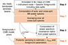 |
Fig. 1. Schematic of pipeline A. Orange colors mark steps that are repeated 500 times, once for each simulation. |
In step 1, power spectra are measured using a pseudo-Cℓ approach with B-mode purification as implemented in NaMaster (Alonso et al. 2019), accounting for the leakage of E-mode power into B-mode power caused by incomplete sky coverage. As described in Smith & Zaldarriaga (2007) the presence of a sky mask leads to the presence of ambiguous modes contaminated by full-sky E-modes. These must be removed at the map level to avoid the contribution to the power spectrum uncertainties from the leaked E-modes. The mask used for this analysis traces the hits count map released in SO Collaboration (2019) (see Fig. 2), and its edges are apodized using a C1-type kernel (see Grain et al. 2009) with an apodization scale of 10 degrees, yielding an effective sky coverage of fsky ∼ 10%. Each power spectrum is calculated in bandpower windows with constant bin width Δℓ = 10, of which we only keep the range 30 ≤ ℓ ≤ 300. Our assumption is that on real data, larger scales are contaminated by atmospheric noise and filtering, whereas smaller scales, targeted by the SO-LAT and useful for constraining lensing B-modes, do not contain any significant primordial B-mode contribution. To avoid a significant bias in the auto-correlations when removing the impact of instrumental noise, a precise noise model is required that may not be available in practice. We address this issue by using data splits, which in the case of real data may be formed by subdividing data among observation periods, sets of detectors, sky patches, or by other means, while in this paper, we resort to simulations.
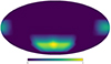 |
Fig. 2. Apodized SAT hits map with effective fsky = 10% used in this paper, shown in equatorial projection. Mask edges are apodized using a C1-type kernel with an apodization scale of 10 degrees. |
We construct simulated observations for each sky realization comprising S = 4 independent splits with the same sky but different noise realizations (each with a commensurately larger noise amplitude). We compute BB power spectra from pairs of maps, each associated with a given data split and a given frequency channel. For any fixed channel pair combination, we average over the corresponding set of S(S − 1)/2 = 6 power spectra with unequal split pairings. For N = 6 SAT frequency channels, this results in a collection of N(N + 1)/2 = 21 noise-debiased multi-frequency power spectra, shown in Fig. 3. We note that, in principle, we could model and subtract the noise bias explicitly, since we have full control over the noise properties in our simulations. In realistic settings, however, the accuracy of an assumed noise model may be limited. While inaccurate noise modeling would affect the statistical uncertainty σ(r) through the covariance matrix calculated from simulations, the cross-split approach ensures robustness of the inferred value of r against noise-induced bias.
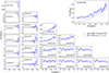 |
Fig. 3. Simulated power spectrum input data analyzed by pipeline A. We show a single realization of CMB and Gaussian foregrounds. Blue shaded areas quantify the 1σ Gaussian standard deviation calculated from simulations of CMB, noise, and Gaussian foregrounds. We note that negative auto-spectra can occur at noise-dominated scales as a result of cross-correlating data splits. |
In step 2, we estimate the bandpower covariance matrix from simulations, assuming no correlations between different multipole windows. We note that, since our realistic foreground templates cannot be used as statistical samples, the covariance computation assumes Gaussian foreground simulations (see Sect. 3) to include foreground signal variance in the budget. As we show in Appendix A, this covariance matrix is indeed appropriate, as it leads to the theoretically expected empirical distribution of the  statistic not only in the case of Gaussian foregrounds, but also for the non-Gaussian foreground simulations. Inaccurate covariance estimates would make this statistic peak at higher or lower values, which we do not observe.
Step 3 is the parameter inference stage. We use a Gaussian likelihood when comparing the multi-frequency power spectra with their theoretical prediction. We note that, in general, the power spectrum likelihood is non-Gaussian, and Hamimeche & Lewis (2008) provide an approximate likelihood that is able to account for this non-Gaussianity. We explicitly verified that both likelihoods lead to equivalent parameter constraints, and thus choose the simpler Gaussian option. The validity of the Gaussian approximation is a consequence of the central limit theorem, since each measured bandpower consists of effectively averaging over Nmodes ≃ Δℓ×fsky × (2ℓ+1) > 61 independent squared modes on the scales used here. We note that this assumption is valid thanks to the relatively large SO-SAT sky patch and would not hold any longer for the smaller BICEP/Keck-like patch sizes. The default sky model is the same as that described in Abitbol et al. (2021). We model the angular power spectra of dust and synchrotron as power laws of the form Dℓ = Ac(ℓ/ℓ0)αc, with ℓ0 = 80, and c = d or s for dust and synchrotron, respectively. The dust SED is modeled as a modified black-body spectrum with spectral index βd and temperature Θd, which we fix to Θd = 20 K. The synchrotron SED is modeled as a power law with spectral index βs. Finally, we consider a dust-synchrotron correlation parameter ϵds. Including the tensor-to-scalar ratio r and a free lensing B-mode amplitude Alens, this fiducial model has nine free parameters:
 (1)
(1)
We refer to this method as “Cℓ-fiducial”. Table 2 lists the priors on its parameters.
Parameter priors for pipeline A, considering both the Cℓ-fiducial model and the Cℓ-moments model.
The main drawback of power-spectrum-based pipelines in their simplest incarnation, is their inability to account for spatial variation in the foreground spectra. If ignored, this spatial variation can lead to biases at the level of r ∼ O(10−3), which are significant for the SO target. At the power spectrum level, spatially-varying SEDs give rise to frequency decorrelation, which can be included in the model. In this work, we show results for an extended model that uses the moment-based3 parameterization of Azzoni et al. (2021) to describe the spatial variation of βd and βs. The model introduces four new parameters
 (2)
(2)
where Bc parameterizes the amplitude of the spatial variations in the spectral index of component c, and γc is their power spectrum slope (see Azzoni et al. 2021, for further details). We refer to results using this method as “Cℓ-moments”, or “A + moments”. The priors in the shared parameter space are the same as for Cℓ-fiducial. Table 2 lists the priors on its additional four parameters. For both methods, we sample posteriors using the emcee code (Foreman-Mackey et al. 2013). It should be noted that we assume a top-hat prior on r in the range [ − 0.1, 0.1] instead of imposing r > 0. The reason is that we would like to remain sensitive to potential negative biases on r. While negative r values do not make sense physically, they may result from volume effects caused by choosing specific priors on other parameters that we marginalize over. Opening the prior on r to negative values allows us to monitor these unwanted effects, offering a simple robustness check. On real data, this will be replaced by a positivity prior r > 0, but only after ensuring that our specific prior choices on the other parameters do not bias r, which is the focus of future work.
2.2. Pipeline B: NILC cleaning
Our second pipeline is based on the blind Internal Linear Combination (ILC) method, which assumes no information on foregrounds whatsoever, and instead only assumes that the observed data contains one signal of interest (the CMB), plus noise and contaminants (Bennett et al. 2003). The method assumes a simple model for the observed multi-frequency maps dν at Nν frequency channels (in either pixel or harmonic space)
 (3)
(3)
where aν is the black-body spectrum of the CMB, s is the amplitude of the true CMB signal, and nν is the contamination in channel ν, which includes the foregrounds and instrumental noise. ILC exploits the difference between the black-body spectrum of the CMB and the SED(s) of other components that may be present in the data. The method aims at reconstructing a map of the CMB component  as a linear combination of the data with a set of weights wν allowed to vary across the map,
 (4)
(4)
where both w and  are Nν × Npix matrices, with Npix being the number of pixels. We optimize the weights by minimizing the variance of
  and find
 (5)
(5)
where a is the black-body spectrum of the CMB (i.e., a vector filled with ones if maps are in thermodynamic temperature units), and  is the frequency-frequency covariance matrix per pixel of the observed data. We do not assume any correlation between pixels in this work.
In our particular implementation, we use the NILC method (Delabrouille et al. 2009; Basak & Delabrouille 2012, 2013). NILC uses localization in pixel and harmonic space by finding different weights w for a set of harmonic filters, called “needlet windows”. These windows are defined in harmonic space hi(ℓ) for i = 0, ..., nwindows − 1 and must satisfy the constraint  in order to preserve the power of the reconstructed CMB. We use nwindows = 5 needlet windows shown in Fig. 4, and defined by
 (6)
(6)
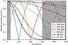 |
Fig. 4. Five needlet windows and beam transfer functions as used in pipeline B. Colored lines are needlet windows in harmonic space, black dashed lines are the transfer functions |

with ℓmin = {0, 0, 100, 200, 350}, ℓmax = {100, 200, 350, 500, 500}, and ℓpeak = {0, 100, 200, 350, 500} for the corresponding five needlet windows. Even though we do not use the full 500-ℓ range where windows are defined for the likelihood sampling, we still perform the component separation on all five windows up to multipoles beyond our upper limit of ℓ = 300, in order to avoid edge effects on the smaller scales.
Let us now describe the NILC procedure as illustrated in Fig. 5. In step 1, we perform our CMB reconstruction in the E and B field instead of Q and U. We transform the observed maps to  with X ∈ E, B. All frequency channels are then brought to a common beam resolution by rescaling the harmonic coefficients with an appropriate harmonic beam window function. The common beam we adopt is the one from the third frequency channel at 93 GHz, which corresponds to a FWHM of 30 arcmin. For each needlet window index i, we multiply
  by hi(ℓ) as a harmonic filter. Since different frequency channels have different limiting resolutions, we do not use all channels in every needlet window. The first two windows use all six frequency channels, the third window does not use the 27 GHz channel, and the last two needlet windows do not use the 27 and 39 GHz channels. The covariance matrix
  has dimensions Nν × Nν × Npix. For each pixel p, its corresponding Nν × Nν elements are computed directly from the data, averaging over the pixels inside a given pixel domain 𝒟(p, i) around each pixel. In practice, the element ν, ν′ of the covariance matrix is calculated by multiplying the two filtered maps at channels ν and ν′, then smoothing that map with a Gaussian kernel with FWHM equal to the size of the pixel domain 𝒟(p, i). The FWHMs for the pixel domain size are 185, 72, 44, 31, and 39 degrees for each needlet window, respectively4.
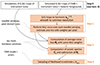 |
Fig. 5. Schematic of pipeline B. Orange colors mark steps that are repeated 500 times, once for each simulation. |
We then proceed to calculate the weights wT (see Eq. (5)) for window i, which is an array with shape (2, Nν,  ), with the first dimension corresponding to the E and B fields. We note that the number of pixels
  is different for each needlet window, since we use different pixel resolutions that depend on the smallest scale covered by the respective window. Finally, we apply Eq. (4) to obtain an ILC-reconstructed CMB map for window i. The final step is to filter this map in harmonic space for a second time with the hi(ℓ) window. The final reconstructed CMB map is the sum of these maps for all five needlet windows.
In step 2, the reconstructed CMB maps are compressed into power spectra using NaMaster and deconvolved to the common beam resolution. We use B-mode purification as implemented in the software and the mask shown in Fig. 2. We estimate the noise bias Nℓ in the final map by computing the power spectrum of noise-only simulations processed with the needlet weights and windows obtained from the simulated data as described above. Nℓ is averaged over simulations and subtracted from the Cℓ of the reconstructed maps.
Finally, in step 3, we run a Monte Carlo Markov Chain (MCMC) over the reconstructed BB spectrum (we ignore EE and EB) with two free parameters, the tensor-to-scalar ratio r and the amplitude of the BB lensing spectrum Alens. For the posterior sampling, we use the Python package emcee. Both parameters have a top hat prior (between 0 and 2 for Alens, and between −0.013 and infinity for r). The covariance matrix is calculated directly over 500 simulations with the same setup but with Gaussian foregrounds. As likelihood, we use the same Gaussian likelihood used in pipeline A and restrict the inference to a multipole range 30 < ℓ ≤ 300.
While the NILC implementation described above is blind, it can be extended to a semi-blind approach that introduces a certain level of foreground modeling. For example, constrained ILC (cILC, Remazeilles et al. 2011) explicitly nullifies one or more contaminants (such as thermal dust) in observed maps, by including their modeled SED in the variance minimization that results in the ILC weights (see Eq. (5)). This foreground modeling can be further extended to include the moment expansion of the SED described in Sect. 2.1. This method, known as constrained moment ILC (cMILC, Remazeilles et al. 2021), has proven effective at cleaning the large-scale B-mode contamination for space experiments such as LiteBIRD. While not used in this work, these extensions and others will be considered in future analyses with more complex foregrounds and systematics.
2.3. Pipeline C: map-based cleaning
Our third pipeline is a map-based parametric pipeline based on the fgbuster code (Poletti & Errard in prep.). This approach is based on the data model
 (7)
(7)
where d is a vector containing the polarized frequency maps, s is a vector containing the Q and U amplitudes of the sky signals (CMB, foregrounds) and n is the noise contained in each frequency map. The matrix  is the so-called mixing matrix, assumed to be parameterized by a set of spectral indices β. Starting from the observed (mock) input data d, Fig. 6 shows a schematic of the pipeline, comprising four steps.
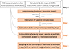 |
Fig. 6. Schematic of pipeline C. Orange colors indicate repetition for each simulation. |
Step 0 is the preprocessing of input simulations. For each simulation, we combine the simulated noise maps, the foreground, and CMB maps and save them on disk. We create a new set of frequency maps,  , smoothed with a common Gaussian kernel of 100′ FWHM.
Step 1 is the actual component separation stage. We optimize the spectral likelihood, defined as (Stompor et al. 2009):
 (8)
(8)
which uses the common resolution frequency maps,  , built during step 0. The right hand side of Eq. (8) contains a sum over the observed sky pixels, assumed to have uncorrelated noise. The diagonal noise covariance matrix
  is computed from 500 noise-only simulations. Although, in principle,
  can be non-diagonal, we do not observe any significant bias of the spectral likelihood due to this approximation in this study. By minimizing Eq. (8) we estimate the best-fit spectral indices
  and the corresponding mixing matrix
  . We also estimate the uncertainties on the recovered spectral indices as provided by the minimizer, a truncated Newton algorithm (Nash 1984) as implemented in scipy (Virtanen et al. 2020). Having thus obtained estimators of the foreground SEDs, we can recover the sky component maps with the generalized least-square equation
 (9)
(9)
where d is the input raw data, and not the common resolution maps. In steps 1 and 2, we have the possibility to use an inhomogeneous noise covariance matrix  and, although this is not exploited in this work, a spatially varying mixing matrix
  . For the latter, one can use the multi-patch or clustering methods implemented in fgbuster (Errard & Stompor 2019; Puglisi et al. 2022).
Step 2 comprises the calculation of angular power spectra. The recovered CMB polarization map is transformed to harmonic space using NaMaster. We estimate an effective transfer function,  , associated with the reconstructed components
  , from the channel-specific beams Bℓ. Correcting for the impact of this effective beam is vital to obtain an unbiased BB power spectrum of the foreground-cleaned CMB,
  . In the second step, we use noise simulations to estimate the noise bias
 (10)
(10)
where  is the noise in the recovered component-separated sky maps. We consider 500 simulations to estimate the noise bias.
Step 3 is the cosmological analysis stage. We model the angular power spectrum of the component-separated CMB map, including the noise contribution, as
 (11)
(11)
and compare data and model with the cosmological likelihood
 (12)
(12)
It is worth noting that this is only an approximation to the true map-level Gaussian likelihood which approximates the effective number of modes in each multipole after masking and purification as fsky(2ℓ+1), thus neglecting any mode-coupling effects induced by the survey footprint. We grid the likelihood above along the two dimensions r and Alens. For each simulation we then estimate the maximum-likelihood values and 68% credible intervals from the marginal distributions of r and Alens. We verified that the distributions of recovered {r, Alens} across simulations are well described by a Gaussian, hence supporting the Gaussian likelihood in Eq. (12).
Pipeline C also offers the option to marginalize over a dust template. The recovered components in  , Eq. (9), include the dust Q and U maps which are typically recovered with high signal-to-noise. In the same way that we compute
  in step 2, we compute the BB component of the recovered dust map,
  . We then update our cosmological likelihood, Eq. (11), by adding a dust term:
 (13)
(13)
This is a similar approach to earlier methods (Errard & Stompor 2019; LiteBIRD Collaboration 2022). When choosing this approach, the inference of r during step 3 therefore involves the marginalization over both parameters Alens and Adust. In principle one could add synchrotron or other terms in Eq. (13) but we limit ourselves to dust as it turns out to be the largest contamination, and, in practice, marginalizing over it allows us to get unbiased estimates of cosmological parameters. In the remainder of this paper, we refer to this method as “C + dust marginalization”.
3. Description of input simulations
We built a set of dedicated simulations against which to test our data analysis pipelines and compare results. The simulated maps include cosmological CMB signal, Galactic foreground emission as well as instrumental noise.
3.1. Instrumental specifications and noise
We simulate polarized Stokes Q and U sky maps as observed by the SO-SAT telescopes. All maps are simulated using the HEALPix pixelation scheme (Górski et al. 2005) with resolution parameter Nside = 512.
We model the SO-SAT noise power spectra as
![Mathematical equation: $$ \begin{aligned} N_{\ell } = N_{\rm white}\left[1+\left(\frac{\ell }{\ell _{\rm knee}}\right)^{\alpha _{\rm knee}}\right], \end{aligned} $$](/articles/aa/full_html/2024/06/aa46105-23/aa46105-23-eq43.gif) (14)
(14)
where Nwhite is the white noise component while ℓknee, and αknee describe the contribution from 1/f noise. Following SO Collaboration (2019; hereinafter SO2019), we consider four scenarios: “baseline” and “goal” levels for the white noise component, and “pessimistic” and “optimistic” correlated noise. The empirical 1/f scenarios are based on measurements from recent experiments and consider polarization modulation, filtering, and atmospheric transmission corresponding to the conditions at the Atacama site. The values of white noise, ℓknee, and αknee associated with the different cases are reported in Table 3. We note that noise levels correspond to a sky fraction of fsky = 10% and five years of observation time, as in SO2019. Differently from SO2019, we cite polarization noise levels at a uniform map coverage, accounting for the factor of ∼1.3 difference compared to Table 1 in SO20195. We simulate noise maps as Gaussian realizations of the Nℓ power spectra. In our main analysis, we use noise maps with pixel weights computed from the SO-SAT hits map (see Fig. 2) and refer to this as “inhomogeneous noise”. In Sect. 4.2, we briefly present results obtained from equally weighted noise pixels, which we refer to as “homogeneous noise”. Otherwise, all results in this paper assume inhomogeneous noise. We note that, although inhomogeneous, the noise realizations used here lack some of the important anisotropic properties of realistic 1/f noise, such as stripes due to the scanning strategy. Thus, together with the impact of other time-domain effects (e.g. filtering), we leave a more thorough study of the impact of instrumental noise properties for future work.
Instrument and noise specifications used to produce the simulations in this work.
3.2. CMB
We simulate the CMB signal as isotropic Gaussian random realizations following a power spectrum computed at the Planck 2018 best-fit ΛCDM cosmology. Our baseline model does not include any primordial tensor signal (r = 0) but incorporates lensing power in the BB spectra (Alens = 1). We consider also two modifications of this model: (i) primordial tensor signal with r = 0.01, representing a ≳3σ target detection for SO with σ(r) = 0.003, as forecasted by SO2019; (ii) reduced lensing power with Alens = 0.5, corresponding to a 50% delensing efficiency, achievable for SO as shown in Namikawa et al. (2022).
For every scenario, we simulated 500 realizations of the CMB signal, convolved with Gaussian beams for each frequency channel, with FWHMs as reported in Table 3.
3.3. Foregrounds
Thermal emission from Galactic dust grains and synchrotron radiation are known to be the two main contaminants to CMB observations in polarization, at intermediate and large angular scales, impacting therefore measurements of the primordial BB signal. The past years have seen many studies on the characterization of polarized Galactic foreground emission, thanks to the analysis of WMAP and Planck data, as well as low frequency surveys (Harper et al. 2022; Krachmalnicoff et al. 2018). However, many aspects of their emission remain unconstrained, including, in particular, the characterization of their SEDs and their corresponding variation across the sky. To properly assess the impact of foreground emission on component separation and r constraints, we therefore use four sets of sky emission models. As specified in the following, we use the Python sky model (PYSM) package (Thorne et al. 2017) to simulate polarized foreground components, with some additional modifications:
Gaussian foregrounds. We simulate thermal dust emission and synchrotron radiation as Gaussian realizations of power law EE and BB power spectra. Although inaccurate, since foregrounds are highly non-Gaussian, this idealistic model was used to validate the different pipelines and to build approximate signal covariance matrices from 500 random realizations. In particular, we estimate the amplitudes of the polarized foreground signal (evaluated for Dℓ = ℓ(ℓ + 1)Cℓ/2π at ℓ = 80) and the slope of angular power spectra from the PYSM synchrotron and thermal dust templates, evaluated at the SO-SAT sky patch. We obtain the following values (d: thermal dust at 353 GHz; s: synchrotron at 23 GHz): 
 ,
, 
 ,
,  ,
,  ;
; 
 ,
, 
 ,
,  ,
,  . This model assumes the frequency scaling of the maps across the SO channels to be a modified black body for thermal dust emission, with fixed spectral parameters βd = 1.54 and Td = 20 K, and a power law for synchrotron with fixed βs = −3 (in antenna temperature units).
d0s0 model. In this case, multi-frequency maps are taken from the d0s0 PYSM model. This model includes templates for thermal dust emission coming from Planck high frequency observations and from WMAP 23 GHz maps from synchrotron radiation. SEDs are considered to be uniform across the sky with the same values of the spectral parameters used for the Gaussian simulations.
d1s1 model. This model uses the same foreground amplitude templates as d0s0, but with the inclusion of spatial variability for spectral parameters, as described in Thorne et al. (2017).
dmsm model. This model represents a modification of the d1s1 spatial variation of spectral parameters. For thermal dust we smoothed the βd and Td templates at an angular resolution of 2 degrees, in order to down-weight the contribution of instrumental noise fluctuations in the original PYSM maps. For synchrotron emission we modified the βs PYSM in order to account for the additional information coming from the analysis of S-PASS data at 2.3 GHz (see Krachmalnicoff et al. 2018). In particular S-PASS data show that the synchrotron spectral index presents enhanced variations with respect to the PYSM template. We therefore multiplied the fluctuations in the βs map by a factor 1.6 to take into consideration larger variations. Moreover, we added small scale fluctuations (with a minimum angular resolution of 2 degrees), as Gaussian realization of a power-law power spectrum with slope −2.6 (see Fig. 11 in Krachmalnicoff et al. 2018).
We note that this set of foreground models generalizes the what was done SO Collaboration (2019), since it includes the d1s1 model, used for large-scale B-mode forecasts in that earlier analysis. As for the CMB simulations, the multi-frequency foreground maps at the SO reference frequencies were convolved with Gaussian beams, to reach the expected angular resolution. We assumed delta-like frequency bandpasses in order to accelerate the production of these simulations, although all pipelines are able to handle finite bandpasses. Therefore this approximation should not impact the performance of any of the pipelines presented here.
4. Results and discussion
Simulations were generated for four different noise and foreground models, respectively, (see Sect. 3), for a total of 16 different foreground-noise combinations. For the main analysis, we consider a fiducial CMB model with Alens = 1 (no delensing) and r = 0 (no primordial tensor fluctuations). In addition, we explored three departures from the fiducial CMB model, with input parameters (Alens = 0.5, r = 0), (Alens = 1, r = 0.01), and (Alens = 0.5, r = 0.01). Here we report the results found for all these cases.
4.1. Power spectra
Let us start by examining the CMB power spectrum products. Pipelines B and C produce CMB-only maps and base their inference of r on the resulting power spectra, whereas pipeline A works directly with the cross-frequency power spectra of the original multi-frequency maps. Nevertheless, CMB power spectra are an important data product that every pipeline should be able to provide. Following the methods presented in Dunkley et al. (2013) and Planck Collaboration XI (2016), Planck Collaboration V (2020), we use a modified version of pipeline A that retrieves CMB-only bandpowers from multi-frequency power spectra, marginalizing over foregrounds with an MCMC sampler as presented in Sect. 2.1. We note that this method, originally developed for high-ℓ CMB science, is applicable since we are in the Gaussian likelihood regime. By re-inserting this cleaned CMB spectrum into a Gaussian likelihood with parameters (r, Alens), we obtain constraints that are consistent with the results shown in Table 4.
Figure 7 shows the CMB power spectra for the three complex foreground simulations d0s0, d1s1, and dmsm (upper, middle, and lower panel, respectively) while considering the goal-optimistic noise scenario. The various markers with error bars denote the measured CMB power spectra and their 1σ standard deviation across 500 simulations, while the black solid line denotes the input CMB power spectrum. Results are shown in gold triangles, blue circles, turquoise diamonds for pipeline A, B, and C respectively. The dotted lines show the best-fit CMB model for the three nominal pipelines (using the same color scheme). Only in the dmsm foreground scenario, which is the most complex considered here, we also show the results from pipeline C + dust marginalization (dark red squares with error bars), and the best-fit CMB power spectrum from A + moments (pink dot-dashed line) and C + dust marginalization (dark red dot-dashed line).
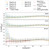 |
Fig. 7. CMB-only power spectra resulting from component separation with pipelines A, B, and C. We show non-Gaussian foregrounds scenarios d0s0 (top panel), d1s1 (middle panel), and dmsm (bottom panel) and consider the goal-optimistic noise scenario. The different colored markers with error bars show the mean of 500 simulations and the scatter between them (corresponding to the statistical uncertainties of a single realization). The dotted lines in the corresponding colors indicate the best-fit power spectrum model. In the dmsm case, we show the extended pipeline results from A + moments and C + dust marginalization with the best-fit models shown as dot-dashed lines. The black solid line is the input CMB model containing lensing B-modes only. We stress that pipeline C only considers multipoles up to ℓ = 180 in the power spectrum likelihood. |
For the nominal pipelines (A, B, and C) without extensions, the measured power spectra display a deviation from the input CMB at low multipoles, increasing with rising foreground complexity. For dmsm at multipoles ≲50, this bias amounts to about 1.5σ and goes down to less than 0.5σ at 80 ≲ ℓ ≲ 250. The three pipelines agree reasonably well, while pipeline A appears slightly less biased for the lowest multipoles. Pipelines B and C show an additional mild excess of power in their highest multipole bins, with a < 0.3σ increase in pipeline C for 130 ≲ ℓ ≲ 170 and up to 1σ for the highest multipole (ℓ = 297) in pipeline B. This might indicate power leakage from the multiple operations on map resolutions implemented in pipelines B and C. In pipeline B, these systematics could come from first deconvolving the multi-frequency maps and then convolving them with a common beam in order to bring them to a common resolution, whereas in pipeline C, the leakage is likely due to the linear combination of the multi-resolution frequency maps following Eq. (9). Other multipole powers lie within the 1σ standard deviation from simulations for all three pipelines.
Both extensions, A + moments and C + dust marginalization, lead to an unbiased CMB power spectrum model, as shown by the pink and dark red dot-dashed lines and the square markers in the lower panel of Fig. 7. In the case of pipelines B and C, comparing the best-fit models obtained from the measured power spectra to the input CMB model, we find sub-sigma bias for all bins with ℓ > 100. We show, however, that the ability to marginalize over additional foreground residuals (e.g. the dust-template marginalization in pipeline C) is able to reduce this bias on all scales, at the cost of increased uncertainties. Implementing this capability in the blind NILC pipeline B would likely allow to reduce the bias that we see.
The SO-SATs are expected to constrain the amplitude of CMB lensing B-modes to an unprecedented precision. As can be seen from Fig. 7, individual, cleaned CMB bandpowers without delensing at multipoles ℓ ≳ 150 achieve a signal-to-noise ratio of about 10, accounting for a combined precision on the lensing amplitude of σ(Alens)≲0.03 when considering multipoles up to ℓmax = 300. As we show in the following section, this is consistent with the inference results obtained by pipelines A and B.
4.2. Constraints on r
Having presented the results on the CMB power spectra, let us now examine the final constraints on r obtained by each pipeline applied to 500 simulations. These results are summarized in Fig. 8 and Table 4. Figure 8 shows the mean r and (16, 84)% credible intervals found by each pipeline as a function of the input foreground model (labels on the x axis). Results are shown for five pipeline setups: pipeline A using the Cℓ-fiducial model (red), pipeline A using the Cℓ-moments model (yellow), pipeline B (blue), pipeline C (green), and pipeline C including the marginalization over the dust amplitude parameter (cyan). For each pipeline, we show two points with error bars. The dot markers and smaller error bars correspond to the results found in the best-case instrument scenario (goal noise level, optimistic 1/f component), while the cross markers and larger error bars correspond to the baseline noise level and pessimistic 1/f component. The quantitative results are reported in Table 4.
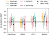 |
Fig. 8. Mean r with (16, 84)% credible interval from 500 simulations. We apply the three nominal component separation pipelines (plus extensions) to simulations with four foreground scenarios of increasing complexity. We assume a fiducial cosmology with r = 0 and Alens = 1, inhomogeneous noise with goal sensitivity and optimistic 1/f noise component (dot markers), and inhomogeneous noise with baseline sensitivity and pessimistic 1/f noise component (cross markers). We note that the NILC results for Gaussian foregrounds are based on a smaller sky mask, see Appendix B. |
We start by discussing the nominal pipelines A, B, and C without considering any extensions. We find that for the simpler Gaussian and d0s0 foregrounds, the nominal pipelines obtain unbiased results, as expected. Pipeline B shows a slight positive bias for Gaussian foregrounds, in combination with inhomogeneous noise only. This bias is absent for homogeneous noise and can be traced back to the pixel covariance matrix used to construct the NILC weights. We discuss this in more detail in Appendix B. For now, we show the results using a smaller, more homogeneously weighted mask. We stress that these results, marked with a †, are not comparable to the rest in Table 4, since they are calculated on a different mask. The more complex d1s1 foregrounds lead to a ∼1σ bias in the goal and optimistic noise scenario. The dmsm foregrounds lead to a noticeable increase of the bias of up to ∼2σ, seen with pipeline C in all noise scenarios and with pipeline A in the goal-optimistic case, and slightly less with pipeline B. The modifications introduced in the dmsm foreground model include a larger spatial variation in the synchrotron spectral index βs with respect to d1s1, and are a plausible reason for the increased bias on r.
Remarkably, we find that, in their simplest incarnation, all pipelines achieve comparable statistical uncertainty on r, ranging from σ(r)≃2.1 × 10⁻³ to σ(r)≃3.6 × 10⁻³ (a 70% increase), depending on the noise model. Changing between the goal and baseline white noise levels results in an increase of σ(r) of ∼20 − 30%. Changing between the optimistic and pessimistic 1/f noise has a similar effect on the results from pipelines A and B, although σ(r) does not increase by more than 10% when changing to pessimistic 1/f noise for pipeline C. These results are in reasonable agreement with the forecasts presented in SO Collaboration (2019).
Let us now discuss the pipeline extensions A + moments and C + dust marginalization. Notably, in all noise and foreground scenarios, the two extensions are able to reduce the bias on r to below 1σ. For the Gaussian and d0s0 foregrounds, we consistently observe a small negative bias (at the ∼0.1σ level for A + moments and < 0.5σ for C + dust marginalization). This bias may be caused by the introduction of extra parameters that are prior dominated, like the dust template’s amplitude in the absence of residual dust contamination, or the moment parameters in the absence of varying spectral indices of foregrounds. If those extra parameters are weakly degenerate with the tensor-to-scalar ratio, the marginal r posterior will shift according to the choice of the prior on the extra parameters. The observed shifts in the tensor-to-scalar ratio and their possible relation with these volume effects will be investigated in a future work. For the more complex d1s1 and dmsm, both pipeline extensions effectively remove the bias observed in the nominal pipelines, achieving a ∼0.5σ bias and lower.
The statistical uncertainty σ(r) increases for both pipeline extensions, although by largely different factors. While C + dust marginalization yields σ(r) between 3.0 × 10⁻³ and 5.9 × 10⁻³, the loss in precision for A + moments is significantly smaller, with σ(r) varying between 2.7 × 10⁻³ and 4.0 × 10⁻³ depending on the noise scenario, an average increase of ∼25% compared to pipeline A. In any case, within the assumptions made regarding the SO noise properties, it should be possible to detect a primordial B-mode signal with r = 0.01 at the 2–3σ level with no delensing. The impact of other effects, such as time domain filtering or anisotropic noise may affect these forecasts, and will be studied in more detail in the future.
We repeated this analysis for input CMB maps generated assuming either r = 0 or 0.01, and either Alens = 0.5 or 1. For simplicity, in these cases we considered only the baseline white noise level with optimistic 1/f noise and the moderately complex d1s1 foreground model. We show results in Fig. 9 and Table 5. A 50% delensing efficiency results in a reduction in the final σ(r) by 25–30% for pipelines A and B, ∼10-20% for A + moments, and 0-33% for C + dust marginalization. The presence of primordial B-modes with a detectable amplitude increases the contribution from cosmic variance to the error budget, with σ(r) growing by up to 40% if r = 0.01, in agreement with theoretical expectations. Using C + dust marginalization and considering no delensing, we even find σ(r) decreasing, hinting at the possible breaking of the degeneracy between r and Adust. We conclude that all pipelines are able to detect the r = 0.01 signal at the level of ∼3σ. As before, we observe a 0.5–1.2σ bias on the recovered r that is eliminated by both the moment expansion method and the dust marginalization method.
Mean r with (16, 84)% credible interval from 500 simulations, using the three nominal pipelines with extensions.
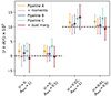 |
Fig. 9. Mean r and (16, 84)% credible interval from 500 simulations, using the three nominal pipelines plus extensions. We assume input models including primordial B-modes and 50% delensing efficiency, the SO baseline noise level with optimistic 1/f component, and the d1s1 foreground template. |
Finally, we explored how cosmological constraints and the pipelines’ performances are affected by noise inhomogeneity resulting from weighting the noise pixels according to the SO-SAT hits map. The geographical location of SO and the size of the SAT field of view constrain possible scanning strategies. In particular, SO must target a patch that has a relatively large sky fraction fsky ∼ 0.15 and is surrounded by a ∼10 degree wide boundary with significantly higher noise (see hits map in Fig. 2). The lower panel of Fig. 10 shows the ratio between the values of σ(r) found using inhomogeneous noise realizations and those with homogeneous noise in the baseline-optimistic noise model with d0s0 foregrounds, averaged over 500 simulations. We see that for all pipeline scenarios, σ(r) increases by ∼30% due to the noise inhomogeneity.
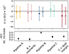 |
Fig. 10. Mean r with (16, 84)% credible intervals from 500 simulations, applying the three nominal component separation pipelines plus extensions. We assume the d0s0 foreground scenario with baseline white noise level and optimistic 1/f component. Cross markers with smaller error bars correspond to homogeneous noise across the SAT field of view and dot markers with larger error bars correspond to inhomogeneous noise. The relative increase in σ(r) between both is shown in the bottom panel. |
4.3. Channel weights
Our three baseline pipelines differ fundamentally in how they separate the sky components. One common feature among all pipelines is the use of six frequency channels to distinguish components by means of their different SEDs. In Fig. 11 we visualize the channel weights as a function of the band center frequency, showing the pipelines in three vertically stacked panels. In the upper panel, we show the effective weights for the CMB applied to the noise-debiased raw power spectra used by pipeline A, distinguishing between weights for each harmonic bin:
 (15)
(15)
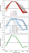 |
Fig. 11. Channel-specific weights associated with the component-separated CMB for the three nominal pipelines. We show the SMICA weights for 27 different ℓ-bins calculated from raw, noisy Cℓs (pipeline A, upper panel), pixel-averaged NILC weights for five needlet windows (pipeline B, middle panel), and pixel-averaged weights from parametric map-based component separation (pipeline C, lower panel). Weights are averaged over 100 simulations, shown are goal white + optimistic 1/f noise (dashed lines) as well as baseline white + pessimistic 1/f noise (solid lines). The semitransparent gray areas represent the channel weights’ 1-σ standard deviation across 100 simulations, covering baseline + pessimistic noise. |
Here,  is the 6 × 6 matrix of raw cross-frequency power spectra from noisy sky maps, a is a vector of length six, filled with ones. This is equivalent to the weights employed by the SMICA component separation method (Cardoso et al. 2008) and by ILC as explained in Sect. 2.2. The middle panel shows the pixel-averaged NILC weights for the five needlet windows (Fig. 4) used in pipeline B. In the lower panel, we show the CMB weights calculated with the map-based component separation, pipeline C, averaged over the observed pixels to yield an array of six numbers. We averaged all channel weights over 100 simulations containing CMB (r = 0, Alens = 1), d1s1 foregrounds, and one of two noise models: goal white noise with optimistic 1/f noise is shown as dashed lines, whereas baseline white noise with pessimistic 1/f noise is shown as solid lines. Moreover, the gray shaded areas quantify the 1-σ uncertainty region of these weights in the baseline-pessimistic case estimated from 100 simulations. We see from Fig. 11 that the average channel weights agree well between pipelines A, B, and C. Mid-frequency channels at 93 and 145 GHz are assigned positive CMB weights throughout all pipelines, while high- and low-frequency channels tend to be suppressed owing to a larger dust and synchrotron contamination, respectively. More specifically, the 280 GHz channel is given negative weight in all pipelines, while average weights at 27, 39, and 225 GHz are negative with pipeline C and either positive or negative in pipelines A and B, depending on the angular scale. The CMB channel weight tends to consistently increase for pipelines A and B as a function of multipole, a fact well exemplified by NILC at 225 GHz, matching the expectation that the CMB lensing signal becomes more important at high ℓ. Overall, Fig. 11 illustrates that foregrounds at low and high frequencies are consistently subtracted by the three component separation pipelines, with the expected scale dependence in pipelines A and B. Moreover, at every frequency, the channel weights are non-negligible and of similar size across the pipelines, meaning that all channels give a relevant contribution to component separation for all pipelines.
4.4. More complex foregrounds: d10s5
During the completion of this paper, the new PYSM3 Galactic foreground models6 were made publicly available. In particular, in these new models, templates for polarized thermal dust and synchrotron radiation were updated including the following changes:
-
Large-scale thermal dust emission is based on the GNILC maps (Planck Collaboration IV 2020), which present a lower contamination from CIB emission with respect to the d1 model, based on Commander templates.
-
For both thermal dust and synchrotron radiation, small scale structures are added by modifying the logarithm of the polarization fraction tensor7.
-
Thermal dust spectral parameters are based on GNILC products, with larger variation of βd and Td parameter at low resolution compared to the d1 model. Small-scale structure is also added as Gaussian realizations of power-law power spectra.
-
The new template for βs includes information from the analysis of S-PASS data (Krachmalnicoff et al. 2018), in a similar way as the one of the sm model adopted in this work. In addition, small-scale structures are present at sub-degree angular scales.
These modifications are encoded in the models called d10 and s5 in the updated version of PYSM. Although these models are still to be considered preliminary, both in terms of their implementation details in PYSM8 and in general, being based on datasets that may not fully involve the unknown level of foreground complexity, we decided to dedicate an extra section to their analysis. For computational speed, we ran the five pipeline set-ups on a reduced set of 100 simulations containing the new d10s5 foregrounds template, CMB with a standard cosmology (r = 0, Alens = 1) and inhomogeneous noise in the goal-optimistic scenario. The resulting marginalized posterior mean and (16, 84)% credible intervals on r, averaged over 100 simulations, are:
 (16)
(16)
We note that the respective bias obtained with pipelines A, B, and C are at 10, 8, and 8σ, at least quadrupling the bias of the dmsm foreground model. Crucially, this bias is reduced to less than 1σ with the A + moments pipeline, with 45% increase in σ(r) compared to pipeline A, and 0.3σ with the C + dust-marginalization pipeline, with a 95% increase in σ(r) compared to pipeline C. This makes A + moments the unbiased method with the lowest statistical error.
The Cℓ-fiducial model achieves minimum χ2 values of 601 ± 41. Although this is an increase of Δχ2 ∼ 30 with respect to the less complex foreground simulations (see Appendix A), the associated probability to exceed (PTE) is 0.10 (assuming our null distribution is a χ2 with Ndata − Nparameters = 558 degrees of freedom), and therefore it would not be possible to identify the presence of a foreground bias by virtue of the model providing a bad fit to the data. The minimum χ2 values we find also confirm that the covariance matrix calculated from Gaussian simulations is still appropriate for the non-Gaussian d10s5 template. On the other hand, A + moments achieves minimum χ2 values of 537 ± 33, which is about 4% lower than for less complex foreground simulations, indicating an improved fitting accuracy.
As shown in Fig. 12, the relative model odds between Cℓ-fiducial and Cℓ-moments (see Appendix A for more details) vary between 10−26 and 10−2, clearly favoring Cℓ-moments. Out of 100 d10s5 simulations, 99 yield model odds below 1% and 78 below 10−5. As opposed to the less complex foreground simulations (d0s0, d1s1, and dmsm), d10s5 gives strong preference to using the moment expansion in the power spectrum model. We note that the AIC-based model odds are computed from the differences of χ2 values that stem from the same simulation seed and are therefore insensitive to bias from noise and cosmic variance. This explains why AIC odds are the more powerful model comparison tool when compared with the χ2 analysis presented above.
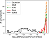 |
Fig. 12. Empirical distribution of the AIC-based relative model odds between the Cℓ-fiducial and the Cℓ-moments model from 100 simulations. We compare five different Galactic foreground templates, including the PYSM foreground model d10s5. Negative values indicate preference for the moments model. We find strong preference for the Cℓ-moments model in the d10s5 foreground scenario, and only then. |
These results consider only the most optimistic noise scenario. Other cases would likely lead to larger uncertainty and, as a consequence, lower relative biases. In this regard, it is highly encouraging to see two pipeline extensions being able to robustly separate the cosmological signal from Galactic synchrotron and dust emission with this high-level complexity. This highlights the importance of accounting for and marginalizing over residual foreground contamination due to frequency decorrelation for the level of sensitivity that SO and other next-generation observatories will achieve.
The contrast between the results obtained on the dmsm and d10s5 simulations gives us an opportunity to reflect on the strategy one should follow when determining the fiducial component separation method to use in primordial B-mode searches. Although the dmsm model leads to a ∼2σ bias on r under the simplest component separation algorithms, simple model-selection metrics are not able to provide significant evidence that a more sophisticated modeling of foregrounds is needed. The situation changes with d10s5. A conservative approach is therefore to select the level of complexity needed for component separation by ensuring that unbiased constraints are obtained for all existing foreground models consistent with currently available data. The analysis methods passing this test can then form the basis for the fiducial B-mode constraints. Alternative results can then be obtained with less conservative component separation techniques, but their goodness of fit (or any similar model selection metric) should be compared with that of the fiducial methods. These results should also be accompanied by a comprehensive set of robustness tests able to identify signatures of foreground contamination in the data. This will form the basis of a future work. In a follow-up paper, we will also explore the new set of complex PYSM3 foreground templates in more detail.
5. Conclusions
In this paper, we present three different component separation pipelines designed to place constraints on the amplitude of cosmological B-modes on polarized maps of the SO Small Aperture Telescopes. The pipelines are based on multi-frequency Cℓ parametric cleaning (Pipeline A), blind Needlet ILC cleaning (Pipeline B), and map-based parametric cleaning (Pipeline C). We also introduce extensions of pipelines A and C that marginalize over additional residual foreground contamination, using a moment expansion or a dust power spectrum template, respectively. We tested and compared their performance on a set of simulated maps containing lensing B-modes with different scenarios of instrumental noise and Galactic foreground complexity. The presence of additional instrumental complexity, such as time-domain filtering, or anisotropic noise, are likely to affect our results. The impact of these effects will be more thoroughly studied in future work.
We find the inferred uncertainty on the tensor-to-scalar ratio σ(r) to be compatible between the three pipelines. While the simpler foreground scenarios (Gaussian, d0s0) do not bias r, spectral index variations can cause an increased bias of 1–2σ if left untreated, as seen with more complex foreground scenarios (d1s1, dmsm). Modeling and marginalizing over the spectral residuals is vital to obtain unbiased B-mode estimates. The extensions to pipelines A and C are able to yield unbiased estimates on all foreground scenarios, albeit with a respective increase in σ(r) by ∼20% (A + moments) and > 30% (C + dust marginalization). These results are in good agreement with the forecasts presented in SO Collaboration (2019).
After testing on simulations with an r = 0.01 cosmology, we conclude that under realistic conditions and if the forecasted map noise levels and characteristics are achieved, SO should be able to detect a r = 0.01 signal at ∼2–3σ after five years of observation. Inhomogeneous noise from the SAT map-making scanning strategy brings about 30% increase in σ(r) as compared to homogeneous noise. Analyzing the per-channel weights for our pipelines, we find all frequency channels to be relevant for the CMB signal extraction and all pipelines to be in good agreement. These forecasts cover the nominal SO survey, and can be considered pessimistic in the light of prospective additional SATs that will further improve the sensitivity on large angular scales.
We also carried out a preliminary analysis of new, more complex, foreground models recently implemented in PYSM3, in particular the d10s5 foreground template. The much higher level of spatial SED variation allowed by this model leads to a drastic increase in the bias on r by up to 10σ, when analyzed with the nominal pipelines A, B, and C. Fortunately, this bias can be reduced to below 1σ when using A + moments and C + dust marginalization. These extensions lead to a 45% and 95% degradation of the error bars, respectively. Our results highlight the importance of marginalizing over residuals caused by frequency decorrelation for SO-like sensitivities. Although our analysis of d10s5 is less exhaustive than that of the other foreground models presented here, it is encouraging to confirm that we have the tools at hand to obtain robust, unbiased constraints on the tensor-to-scalar ratio in the presence of such complex Galactic foregrounds. In addition to the algorithmic improvements presented in this paper, the inclusion of external data sets such as FYST/CCAT-Prime (CCAT-Prime Collaboration 2022) may prove helpful at mitigating foregrounds.
In preparation for the data collected by SO in the near future, we will continue our investigations into Galactic foreground models with other levels of complexity as the field progresses. Nevertheless, the current work shows that the analysis pipelines in place for SO are able to obtain robust constraints on the amplitude of primordial B modes in the presence of Galactic foregrounds covering the full range of complexity envisaged by current, state-of-the-art models.
We note that the pipelines are still agnostic to some aspects of the instrumental noise such as filtering, which may impact the overall forecasted scientific performance. We anticipate studying these in detail in future work.
See Tegmark (1998), Chluba et al. (2017), Vacher et al. (2023) for more details on the moment-expansion formalism in the context of CMB foregrounds, and Mangilli et al. (2021) as an alternative power-spectrum-based description.
The domain sizes are estimated directly from the needlet window scale (see details in the Appendix A of Delabrouille et al. 2009). The ILC bias can be minimized by enlarging the pixel domains to be big enough to include a higher number of modes. We choose the resulting ILC bias to not exceed 0.2%, for which we need pixel domain sizes large enough so that each needlet window contains at least 2500 modes.
Polarization noise accounts for a factor of  and homogeneous noise for a factor of
  compared to Table 1 in SO2019.
The PYSM library is currently under development, with beta versions including minor modifications of the foreground templates being realized regularly. In this part of our analysis we make use of PYSM V3.4.0B3.
Acknowledgments
The authors would like to thank Ken Ganga, Arthur Kosowsky, and the anonymous referee for useful feedback. The group at SISSA acknowledges support from the COSMOS Network of the Italian Space Agency and the InDark Initiative of the National Institute for Nuclear Physics (INFN). KW is funded by a SISSA PhD fellowship. SA is funded by a Kavli/IPMU doctoral studentship. CHC acknowledges NSF award 1815887 and FONDECYT Postdoc fellowship 3220255. DA is supported by the Science and Technology Facilities Council through an Ernest Rutherford Fellowship, grant reference ST/P004474. This work is part of a project that has received funding from the European Research Council (ERC) under the European Union’s Horizon 2020 research and innovation program (PI: Josquin Errard, Grant agreement No. 101044073). ABL is a BCCP fellow at UC Berkeley and Lawrence Berkeley National Laboratory. MLB acknowledges funding from UKRI and STFC (Grant awards ST/X006344/1 and ST/X006336/1). EC acknowledges support from the European Research Council (ERC) under the European Union’s Horizon 2020 research and innovation programme (Grant agreement No. 849169). JC was furthermore supported by the ERC Consolidator Grant CMBSPEC (No. 725456) and the Royal Society as a Royal Society University Research Fellow at the University of Manchester, UK (No. URF/R/191023). GF acknowledges the support of the European Research Council under the Marie Skłodowska Curie actions through the Individual Global Fellowship No. 892401 PiCOGAMBAS. We acknowledge the use of CAMB (Lewis et al. 2000), healpy (Zonca et al. 2019), numpy (Harris 2020), matplotlib (Hunter 2007), emcee (Foreman-Mackey et al. 2013), and fgbuster (Errard & Stompor 2019; Puglisi et al. 2022) software packages.
References
- Abazajian, K. N., Adshead, P., Ahmed, Z., et al. 2016, arXiv e-prints [arXiv:1610.02743] [Google Scholar]
- Abbott, L. F., & Wise, M. B. 1984, Nucl. Phys. B, 244, 541 [Google Scholar]
- Abitbol, M. H., Alonso, D., Simon, S. M., et al. 2021, JCAP, 2021, 032 [CrossRef] [Google Scholar]
- Akaike, H. 1974, IEEE Trans. Autom. Control, 19, 716 [Google Scholar]
- Alonso, D., Dunkley, J., Thorne, B., & Næss, S. 2017, Phys. Rev. D, 95, 043504 [NASA ADS] [CrossRef] [Google Scholar]
- Alonso, D., Sanchez, J., Slosar, A., & LSST Dark Energy Science Collaboration 2019, MNRAS, 484, 4127 [NASA ADS] [CrossRef] [Google Scholar]
- Armitage-Caplan, C., Dunkley, J., Eriksen, H. K., & Dickinson, C. 2012, MNRAS, 424, 1914 [NASA ADS] [CrossRef] [Google Scholar]
- Azzoni, S., Abitbol, M. H., Alonso, D., et al. 2021, JCAP, 2021, 047 [CrossRef] [Google Scholar]
- Basak, S., & Delabrouille, J. 2012, MNRAS, 419, 1163 [Google Scholar]
- Basak, S., & Delabrouille, J. 2013, MNRAS, 435, 18 [Google Scholar]
- Bennett, C. L., Hill, R. S., Hinshaw, G., et al. 2003, ApJS, 148, 97 [Google Scholar]
- Betoule, M., Pierpaoli, E., Delabrouille, J., Le Jeune, M., & Cardoso, J. F. 2009, A&A, 503, 691 [NASA ADS] [CrossRef] [EDP Sciences] [Google Scholar]
- BICEP2 Collaboration& Keck Array Collaboration 2016, Phys. Rev. Lett., 116, 031302 [Google Scholar]
- BICEP2 Collaboration& Keck Array Collaboration 2018, Phys. Rev. Lett., 121, 221301 [Google Scholar]
- BICEP/Keck Collaboration 2021, Phys. Rev. Lett., 127, 151301 [NASA ADS] [CrossRef] [Google Scholar]
- Bonaldi, A., & Ricciardi, S. 2011, MNRAS, 414, 615 [NASA ADS] [CrossRef] [Google Scholar]
- Cardoso, J. F., Martin, M., Delabrouille, J., Betoule, M., & Patanchon, G. 2008, arXiv e-prints [arXiv:0803.1814] [Google Scholar]
- CCAT-Prime Collaboration (Aravena, M., et al.) 2022, ApJS, 264, 7 [NASA ADS] [Google Scholar]
- Chluba, J., Hill, J. C., & Abitbol, M. H. 2017, MNRAS, 472, 1195 [NASA ADS] [CrossRef] [Google Scholar]
- CMB-S4 Collaboration 2022, ApJ, 926, 54 [CrossRef] [Google Scholar]
- Delabrouille, J., & Cardoso, J. F. 2007, International Summer School on Data Analysis in Cosmology (Valencia, Spain, cel-00162531.), 47 [Google Scholar]
- Delabrouille, J., Cardoso, J. F., Le Jeune, M., et al. 2009, A&A, 493, 835 [NASA ADS] [CrossRef] [EDP Sciences] [Google Scholar]
- Dunkley, J., Calabrese, E., Sievers, J., et al. 2013, JCAP, 07, 025 [CrossRef] [Google Scholar]
- Errard, J., & Stompor, R. 2012, Phys. Rev. D, 85, 083006 [NASA ADS] [CrossRef] [Google Scholar]
- Errard, J., & Stompor, R. 2019, Phys. Rev. D, 99, 043529 [NASA ADS] [CrossRef] [Google Scholar]
- Errard, J., Feeney, S. M., Peiris, H. V., & Jaffe, A. H. 2016, JCAP, 2016, 052 [CrossRef] [Google Scholar]
- Foreman-Mackey, D., Hogg, D. W., Lang, D., & Goodman, J. 2013, PASP, 125, 306 [Google Scholar]
- Górski, K. M., Hivon, E., Banday, A. J., et al. 2005, ApJ, 622, 759 [Google Scholar]
- Grain, J., Tristram, M., & Stompor, R. 2009, Phys. Rev. D, 79, 123515 [Google Scholar]
- Hamimeche, S., & Lewis, A. 2008, Phys. Rev. D, 77, 103013 [NASA ADS] [CrossRef] [Google Scholar]
- Harper, S. E., Dickinson, C., Barr, A., et al. 2022, MNRAS, 513, 5900 [NASA ADS] [CrossRef] [Google Scholar]
- Harris, C. R., Millman,K. J., van der Walt, S. J., et al. 2020, Nature, 585, 357 [NASA ADS] [CrossRef] [Google Scholar]
- Hazumi, M., Ade, P. A. R., Akiba, Y., et al. 2019, J. Low Temp. Phys., 194, 443 [Google Scholar]
- Hervías-Caimapo, C., Bonaldi, A., & Brown, M. L. 2017, MNRAS, 468, 4408 [CrossRef] [Google Scholar]
- Hervías-Caimapo, C., Bonaldi, A., Brown, M. L., & Huffenberger, K. M. 2022, ApJ, 924, 11 [CrossRef] [Google Scholar]
- Hui, H., Ade, P. A. R., Ahmed, Z., et al. 2018, Proc. SPIE Int. Soc. Opt. Eng., 10708 [Google Scholar]
- Hunter, J. D. 2007, Comput. Sci. Eng., 9, 90 [NASA ADS] [CrossRef] [Google Scholar]
- Ijjas, A., & Steinhardt, P. J. 2018, CQG, 35, 135004 [NASA ADS] [CrossRef] [Google Scholar]
- Ijjas, A., & Steinhardt, P. J. 2019, Phys. Lett. B, 795, 666 [NASA ADS] [CrossRef] [Google Scholar]
- Kamionkowski, M., & Kovetz, E. D. 2016, ARA&A, 54, 227 [NASA ADS] [CrossRef] [Google Scholar]
- Kamionkowski, M., Kosowsky, A., & Stebbins, A. 1997, Phys. Rev. Lett., 78, 2058 [Google Scholar]
- Katayama, N., & Komatsu, E. 2011, ApJ, 737, 78 [NASA ADS] [CrossRef] [Google Scholar]
- Krachmalnicoff, N., Baccigalupi, C., Aumont, J., Bersanelli, M., & Mennella, A. 2016, A&A, 588, A65 [NASA ADS] [CrossRef] [EDP Sciences] [Google Scholar]
- Krachmalnicoff, N., Carretti, E., Baccigalupi, C., et al. 2018, A&A, 618, A166 [NASA ADS] [CrossRef] [EDP Sciences] [Google Scholar]
- Leach, S. M., Cardoso, J. F., Baccigalupi, C., et al. 2008, A&A, 491, 597 [NASA ADS] [CrossRef] [EDP Sciences] [Google Scholar]
- Lewis, A., & Challinor, A. 2006, Phys. Rep., 429, 1 [Google Scholar]
- Lewis, A., Challinor, A., & Lasenby, A. 2000, ApJ, 538, 473 [Google Scholar]
- LiteBIRD Collaboration 2022, Prog. Theor. Exp. Phys., ptac150 [Google Scholar]
- Maltoni, M., & Schwetz, T. 2003, Phys. Rev. D, 68, 033020 [NASA ADS] [CrossRef] [Google Scholar]
- Mangilli, A., Aumont, J., Rotti, A., et al. 2021, A&A, 647, A52 [NASA ADS] [CrossRef] [EDP Sciences] [Google Scholar]
- Martin, J., Ringeval, C., Trotta, R., & Vennin, V. 2014a, JCAP, 2014, 039 [Google Scholar]
- Martin, J., Ringeval, C., & Vennin, V. 2014b, Phys. Dark Universe, 5, 75 [CrossRef] [Google Scholar]
- Namikawa, T., Baleato Lizancos, A., Robertson, N., et al. 2022, Phys. Rev. D, 105, 023511 [NASA ADS] [CrossRef] [Google Scholar]
- Nash, S. G. 1984, SIAM J. Numer. Anal., 21, 770 [NASA ADS] [CrossRef] [Google Scholar]
- Natoli, P., Ashdown, M., Banerji, R., et al. 2018, JCAP, 2018, 022 [Google Scholar]
- Pearson, K. 1900, London Edinburgh Dublin Philos. Mag. J. Sci., 50, 157 [Google Scholar]
- Planck Collaboration X. 2016, A&A, 594, A10 [NASA ADS] [CrossRef] [EDP Sciences] [Google Scholar]
- Planck Collaboration XI. 2016, A&A, 594, A11 [NASA ADS] [CrossRef] [EDP Sciences] [Google Scholar]
- Planck Collaboration IV. 2020, A&A, 641, A4 [NASA ADS] [CrossRef] [EDP Sciences] [Google Scholar]
- Planck Collaboration V. 2020, A&A, 641, A5 [NASA ADS] [CrossRef] [EDP Sciences] [Google Scholar]
- Planck Collaboration VI. 2020, A&A, 641, A6 [NASA ADS] [CrossRef] [EDP Sciences] [Google Scholar]
- Planck Collaboration X. 2020, A&A, 641, A10 [NASA ADS] [CrossRef] [EDP Sciences] [Google Scholar]
- Planck Collaboration XI. 2020, A&A, 641, A11 [NASA ADS] [CrossRef] [EDP Sciences] [Google Scholar]
- Planck Collaboration Int. XXX. 2016, A&A, 586, A133 [NASA ADS] [CrossRef] [EDP Sciences] [Google Scholar]
- Puglisi, G., Mihaylov, G., Panopoulou, G. V., et al. 2022, MNRAS, 511, 2052 [NASA ADS] [CrossRef] [Google Scholar]
- Remazeilles, M., Delabrouille, J., & Cardoso, J.-F. 2011, MNRAS, 410, 2481 [Google Scholar]
- Remazeilles, M., Dickinson, C., Eriksen, H. K. K., & Wehus, I. K. 2016, MNRAS, 458, 2032 [Google Scholar]
- Remazeilles, M., Banday, A. J., Baccigalupi, C., et al. 2018a, JCAP, 2018, 023 [Google Scholar]
- Remazeilles, M., Dickinson, C., Eriksen, H. K., & Wehus, I. K. 2018b, MNRAS, 474, 3889 [CrossRef] [Google Scholar]
- Remazeilles, M., Rotti, A., & Chluba, J. 2021, MNRAS, 503, 2478 [NASA ADS] [CrossRef] [Google Scholar]
- Seljak, U. 1997, ApJ, 482, 6 [Google Scholar]
- Seljak, U., & Zaldarriaga, M. 1997, Phys. Rev. Lett., 78, 2054 [Google Scholar]
- Smith, K. M., & Zaldarriaga, M. 2007, Phys. Rev. D, 76, 043001 [Google Scholar]
- SO Collaboration 2019, JCAP, 2019, 056 [CrossRef] [Google Scholar]
- Starobinskiǐ, A. A. 1979, Sov. J. Exp. Theor. Phys. Lett., 30, 682 [Google Scholar]
- Stompor, R., Errard, J., & Poletti, D. 2016, Phys. Rev. D, 94, 083526 [NASA ADS] [CrossRef] [Google Scholar]
- Stompor, R., Leach, S., Stivoli, F., & Baccigalupi, C. 2009, MNRAS, 392, 216 [NASA ADS] [CrossRef] [Google Scholar]
- Tegmark, M. 1998, ApJ, 502, 1 [CrossRef] [Google Scholar]
- Thorne, B., Dunkley, J., Alonso, D., & Næss, S. 2017, MNRAS, 469, 2821 [Google Scholar]
- Thorne, B., Dunkley, J., Alonso, D., et al. 2019, arXiv e-prints [arXiv:1905.08888] [Google Scholar]
- Vacher, L., Aumont, J., Montier, L., et al. 2022, A&A, 660, A111 [NASA ADS] [CrossRef] [EDP Sciences] [Google Scholar]
- Vacher, L., Chluba, J., Aumont, J., Rotti, A., & Montier, L. 2023, A&A, 669, A5 [NASA ADS] [CrossRef] [EDP Sciences] [Google Scholar]
- Virtanen, P., Gommers, R., Oliphant, T. E., et al. 2020, Nat. Methods, 17, 261 [Google Scholar]
- Wagenmakers, E., & Farrell, S. 2004, Psychon Bull. Rev., 11, 192 [Google Scholar]
- Zaldarriaga, M., & Seljak, U. 1997, Phys. Rev. D, 55, 1830 [Google Scholar]
- Zaldarriaga, M., & Seljak, U. 1998, Phys. Rev. D, 58, 023003 [Google Scholar]
- Zonca, A., Singer, L., Lenz, D., et al. 2019, J. Open Source Software, 4, 1298 [Google Scholar]
Appendix A: Validation of power spectra and posteriors
The goodness of fit of the power spectrum likelihood can be assessed by the well-known minimum-χ2 statistic  , with d,
  , and C denoting data, best-fit theory model, and covariance, respectively. We perform this validation for pipeline A only, since it includes the foreground model at the likelihood level. Under the hypothesis of Gaussian data,
  is expected to follow a χ2 distribution with N − P = 558 degrees of freedom (Pearson 1900; Maltoni & Schwetz 2003). When using Gaussian foregrounds, we know that our data are sufficiently Gaussian and the covariance is exact within the MCMC noise level. We compute the
  for 100 simulated data realizations containing standard cosmology (r = 0, Alens = 1), inhomogeneous noise in the goal-optimistic scenario and in four foreground cases (Gaussian, d0s0, d1s1, dmsm), considering both the Cℓ-fiducial and the Cℓ-moments model. The empirical distributions match the theoretical expectation in all cases, showing that the covariance matrix is appropriate, even for non-Gaussian foreground input templates.
We also assess, for each simulation seed, which foreground model is preferred by the simulated data, using the Akaike Information Criterion (AIC, Akaike 1974). We compute the difference  , where Δk = 4 is the number of excess parameters of the Cℓ-moments over Cℓ-fiducial. Following Wagenmakers & Farrell (2004), the number exp(ΔAIC/2) can be interpreted as the relative model odds P(Cℓ-fiducial)/P(Cℓ-moments).
The results are shown in Fig. A.1. The AIC test detects no clear preference for Cℓ-moments over Cℓ-fiducial. Among 100 simulations containing dmsm foregrounds, 30 have model odds below 1, and only a single simulation below 10−2. In case of the dmsm simulation set, this might come as a surprise, considering that the Cℓ-moments model allows to mitigate a 1-2σ bias. We conclude that one must be careful when interpreting < 2σ detections in marginal posterior distributions, as they may be difficult to distinguish from subdominant residual foreground contamination using standard model-comparison techniques. As shown in Sect. 4.4, this situation changes in the presence of input foregrounds that induce a large bias.
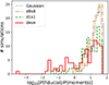 |
Fig. A.1. Empirical distribution of the AIC-based relative model odds between the Cℓ-fiducial and the Cℓ-moments model from 100 simulations. Same as Fig. 12 but only considering the four less complex Galactic foreground templates. Note the different x scale. We do not see strong preference for Cℓ-moments (indicated by large negative values) in any of the cases considered. |
Lastly, we tested the robustness of the statistical results on r quoted in Sect. 4. Using pipelines A, A+moments, and B, we calculated the mean and maximum a-posteriori (MAP) value of the marginal r posterior for each of 500 simulations containing CMB realized with the fiducial cosmology (r = 0, Alens = 1), dmsm foregrounds, and inhomogeneous noise in the baseline-optimistic scenario. We computed the average and standard deviation over the 500 simulations, and repeated the procedure for the lensing amplitude Alens. Table A.1 shows the results. We find that for both parameters and all three pipelines, the sample average of the mean and the MAP agree at the 0.1σ level. We also find consistency between the standard deviation of the marginal posteriors averaged over 500 simulations, the sample scatter of the marginal posterior mean values, and the sample scatter of the MAP values computed from 500 simulations. Table A.1 also lists the Gaussian error on the average mean and MAP values, corresponding to the sample scatter divided by the square root of the number of simulations,  . While this test would result in a bias on r for all component separation pipelines (yet below 2σ in the case of the A + moments pipeline), passing it is far beyond the requirements set by the statistical sensitivity of SO.
Posterior statistics on r and Alens − 1 from 500 simulations. We assume dmsm foregrounds and baseline-optimistic noise, as inferred by the three nominal component separation pipelines. No delensing or primordial gravitational waves are assumed.
Appendix B: Bias on r for Gaussian foregrounds and pipeline B
In the results of pipeline B, we note a consistent bias on r for simulations that include Gaussian foregrounds in combination with inhomogeneous noise. This bias seems unreasonable, considering the results that use more complex foregrounds, such as d0s0, but the same noise and CMB simulations, lead to considerably less bias. The cosmological bias is directly caused by a bias at the large angular scales of the BB power spectrum, which is easily visible when plotting the spectra. We confirm that this bias corresponds to foreground bias. In Fig. B.1 (left panel), we show the reconstructed CMB  spectrum for the standard cosmology (r = 0, Alens = 1) with inhomogeneous goal-pessimistic noise, for both the Gaussian (blue squares) and d0s0 (red squares) foregrounds. The marker and error bar shows the mean and 1-σ standard deviation across the 500 simulations. The excess bias at large scales is evident as the reconstructed CMB clearly surpasses the fiducial BB spectrum. We can calculate the exact foreground bias present on each reconstructed CMB, by mixing the pure foregrounds maps with the same NILC weights (Eq. 5), and taking the power spectra of that foreground bias reconstruction. This is shown as the blue triangles for Gaussian and red triangles for d0s0 foregrounds. In the Gaussian case, we see that the large-scale bias is almost entirely caused by foregrounds.
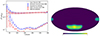 |
Fig. B.1. Foreground bias and custom analysis mask related to needlet-based component separation. Left panel: Foreground residuals in the reconstructed CMB power spectra in the inhomogeneous goal-pessimistic noise scenario, with a fiducial input cosmology of r = 0, Alens = 1, and Gaussian and d0s0 foregrounds. We show the reconstructed CMB and foreground power spectrum residuals |

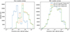 |
Fig. B.2. Distribution of covariance matrix elements used to build the ILC weights (see Eq. 5) for pipeline B. We show values for a single simulation seed used for B-mode reconstruction, and include all cross-frequency combinations. We assume inhomogeneous goal-pessimistic noise, with a fiducial (r = 0, Alens = 1) CMB, with Gaussian, d0s0, and d1s1 foregrounds. Left panel: first needlet window (largest scales), right panel: fifth needlet window (smallest scales). |
We know this bias is directly related to the NILC weights that mix the frequency maps (Eq. 5). The weights are calculated directly from the frequency-frequency covariance matrix, which in turn is calculated from the input frequency maps themselves. If, for instance, we wish to test if the weights calculated with the simulations including Gaussian foregrounds are incorrect, we can do the cross check by using other weights to mix those same frequency maps. We take the NILC weights calculated for the simulations with d0s0 foregrounds (shown in Fig. B.1) and use them to mix the frequency maps that include the Gaussian foregrounds. In this case, the mean best fit is r = −0.0001 ± 0.0026, which is comparable to r = −0.0005 ± 0.0028 for the simulations including d0s0 foregrounds (shown in Table 4).
Any incorrect weights must originate from the NILC covariance matrix. The combination of directly calculating the covariance matrix over maps that have inhomogeneous noise and Gaussian foregrounds creates the observed bias. We can alleviate this problem by spatially constraining the hits mask (Fig. 2) to a more homogeneous area, where the noise map realization will also be more homogeneous. The mask we use to do this is shown in Fig. B.1 (right panel). This custom mask has a smaller sky fraction than the fiducial analysis mask, which increases the statistical uncertainty on the inferred value of r. The measurements using this more constrained and more homogeneous mask are marked with a † in Table 4.
All Tables
Parameter priors for pipeline A, considering both the Cℓ-fiducial model and the Cℓ-moments model.
Instrument and noise specifications used to produce the simulations in this work.
Mean r with (16, 84)% credible interval from 500 simulations, using the three nominal pipelines with extensions.
Posterior statistics on r and Alens − 1 from 500 simulations. We assume dmsm foregrounds and baseline-optimistic noise, as inferred by the three nominal component separation pipelines. No delensing or primordial gravitational waves are assumed.
All Figures
|
Fig. 1. Schematic of pipeline A. Orange colors mark steps that are repeated 500 times, once for each simulation. |
| In the text | |
|
Fig. 2. Apodized SAT hits map with effective fsky = 10% used in this paper, shown in equatorial projection. Mask edges are apodized using a C1-type kernel with an apodization scale of 10 degrees. |
| In the text | |
|
Fig. 3. Simulated power spectrum input data analyzed by pipeline A. We show a single realization of CMB and Gaussian foregrounds. Blue shaded areas quantify the 1σ Gaussian standard deviation calculated from simulations of CMB, noise, and Gaussian foregrounds. We note that negative auto-spectra can occur at noise-dominated scales as a result of cross-correlating data splits. |
| In the text | |
|
Fig. 4. Five needlet windows and beam transfer functions as used in pipeline B. Colored lines are needlet windows in harmonic space, black dashed lines are the transfer functions |
| In the text | |
|
Fig. 5. Schematic of pipeline B. Orange colors mark steps that are repeated 500 times, once for each simulation. |
| In the text | |
|
Fig. 6. Schematic of pipeline C. Orange colors indicate repetition for each simulation. |
| In the text | |
|
Fig. 7. CMB-only power spectra resulting from component separation with pipelines A, B, and C. We show non-Gaussian foregrounds scenarios d0s0 (top panel), d1s1 (middle panel), and dmsm (bottom panel) and consider the goal-optimistic noise scenario. The different colored markers with error bars show the mean of 500 simulations and the scatter between them (corresponding to the statistical uncertainties of a single realization). The dotted lines in the corresponding colors indicate the best-fit power spectrum model. In the dmsm case, we show the extended pipeline results from A + moments and C + dust marginalization with the best-fit models shown as dot-dashed lines. The black solid line is the input CMB model containing lensing B-modes only. We stress that pipeline C only considers multipoles up to ℓ = 180 in the power spectrum likelihood. |
| In the text | |
|
Fig. 8. Mean r with (16, 84)% credible interval from 500 simulations. We apply the three nominal component separation pipelines (plus extensions) to simulations with four foreground scenarios of increasing complexity. We assume a fiducial cosmology with r = 0 and Alens = 1, inhomogeneous noise with goal sensitivity and optimistic 1/f noise component (dot markers), and inhomogeneous noise with baseline sensitivity and pessimistic 1/f noise component (cross markers). We note that the NILC results for Gaussian foregrounds are based on a smaller sky mask, see Appendix B. |
| In the text | |
|
Fig. 9. Mean r and (16, 84)% credible interval from 500 simulations, using the three nominal pipelines plus extensions. We assume input models including primordial B-modes and 50% delensing efficiency, the SO baseline noise level with optimistic 1/f component, and the d1s1 foreground template. |
| In the text | |
|
Fig. 10. Mean r with (16, 84)% credible intervals from 500 simulations, applying the three nominal component separation pipelines plus extensions. We assume the d0s0 foreground scenario with baseline white noise level and optimistic 1/f component. Cross markers with smaller error bars correspond to homogeneous noise across the SAT field of view and dot markers with larger error bars correspond to inhomogeneous noise. The relative increase in σ(r) between both is shown in the bottom panel. |
| In the text | |
|
Fig. 11. Channel-specific weights associated with the component-separated CMB for the three nominal pipelines. We show the SMICA weights for 27 different ℓ-bins calculated from raw, noisy Cℓs (pipeline A, upper panel), pixel-averaged NILC weights for five needlet windows (pipeline B, middle panel), and pixel-averaged weights from parametric map-based component separation (pipeline C, lower panel). Weights are averaged over 100 simulations, shown are goal white + optimistic 1/f noise (dashed lines) as well as baseline white + pessimistic 1/f noise (solid lines). The semitransparent gray areas represent the channel weights’ 1-σ standard deviation across 100 simulations, covering baseline + pessimistic noise. |
| In the text | |
|
Fig. 12. Empirical distribution of the AIC-based relative model odds between the Cℓ-fiducial and the Cℓ-moments model from 100 simulations. We compare five different Galactic foreground templates, including the PYSM foreground model d10s5. Negative values indicate preference for the moments model. We find strong preference for the Cℓ-moments model in the d10s5 foreground scenario, and only then. |
| In the text | |
|
Fig. A.1. Empirical distribution of the AIC-based relative model odds between the Cℓ-fiducial and the Cℓ-moments model from 100 simulations. Same as Fig. 12 but only considering the four less complex Galactic foreground templates. Note the different x scale. We do not see strong preference for Cℓ-moments (indicated by large negative values) in any of the cases considered. |
| In the text | |
|
Fig. B.1. Foreground bias and custom analysis mask related to needlet-based component separation. Left panel: Foreground residuals in the reconstructed CMB power spectra in the inhomogeneous goal-pessimistic noise scenario, with a fiducial input cosmology of r = 0, Alens = 1, and Gaussian and d0s0 foregrounds. We show the reconstructed CMB and foreground power spectrum residuals |
| In the text | |
|
Fig. B.2. Distribution of covariance matrix elements used to build the ILC weights (see Eq. 5) for pipeline B. We show values for a single simulation seed used for B-mode reconstruction, and include all cross-frequency combinations. We assume inhomogeneous goal-pessimistic noise, with a fiducial (r = 0, Alens = 1) CMB, with Gaussian, d0s0, and d1s1 foregrounds. Left panel: first needlet window (largest scales), right panel: fifth needlet window (smallest scales). |
| In the text | |
Current usage metrics show cumulative count of Article Views (full-text article views including HTML views, PDF and ePub downloads, according to the available data) and Abstracts Views on Vision4Press platform.
Data correspond to usage on the plateform after 2015. The current usage metrics is available 48-96 hours after online publication and is updated daily on week days.
Initial download of the metrics may take a while.