| Issue |
A&A
Volume 685, May 2024
|
|
|---|---|---|
| Article Number | A22 | |
| Number of page(s) | 21 | |
| Section | Planets and planetary systems | |
| DOI | https://doi.org/10.1051/0004-6361/202349039 | |
| Published online | 30 April 2024 | |
Accretion of primordial H–He atmospheres in mini-Neptunes: The importance of envelope enrichment
1
Institut für Astrophysik, Universität Zürich,
Winterthurerstr. 190,
8057
Zürich,
Switzerland
e-mail: marit@ics.uzh.ch
2
Weltraumforschung und Planetologie, Physikalisches Institut, Universität Bern,
Gesellschaftsstrasse 6,
3012
Bern,
Switzerland
Received:
20
December
2023
Accepted:
15
February
2024
Context. Out of the more than 5000 detected exoplanets, a considerable number belong to a category called “mini-Neptunes”. Interior models of these planets suggest that they have primordial H–He-dominated atmospheres. As this type of planet is not found in the Solar System, understanding their formation is a key challenge in planet formation theory. Unfortunately, quantifying how much H–He planets have, based on their observed mass and radius, is impossible due to the degeneracy of interior models.
Aims. Another approach to estimating the range of possible primordial envelope masses is to use formation theory. As different assumptions in planet formation can heavily influence the nebular gas accretion rate of small planets, it is unclear how large the envelope of a protoplanet should be. We explore the effects that different assumptions regarding planet formation have on the nebular gas accretion rate, particularly by exploring the way in which solid material interacts with the envelope. This allows us to estimate the range of possible post-formation primordial envelopes. Thereby, we demonstrate the impact of envelope enrichment on the initial primordial envelope, which can be used in evolution models.
Methods. We applied formation models that include different solid accretion rate prescriptions. Our assumption is that mini-Neptunes form beyond the ice line and migrate inward after formation; thus, we formed planets in situ at 3 and 5 au. We considered that the envelope can be enriched by the accreted solids in the form of water. We studied how different assumptions and parameters influence the ratio between the planet’s total mass and the fraction of primordial gas.
Results. The primordial envelope fractions for low- and intermediate-mass planets (total mass below 15 M⊕) can range from 0.1% to 50%. Envelope enrichment can lead to higher primordial mass fractions. We find that the solid accretion rate timescale has the largest influence on the primordial envelope size.
Conclusions. Rates of primordial gas accretion onto small planets can span many orders of magnitude. Planet formation models need to use a self-consistent gas accretion prescription.
Key words: planets and satellites: atmospheres / planets and satellites: composition / planets and satellites: formation
© The Authors 2024
 Open Access article, published by EDP Sciences, under the terms of the Creative Commons Attribution License (https://creativecommons.org/licenses/by/4.0), which permits unrestricted use, distribution, and reproduction in any medium, provided the original work is properly cited.
This article is published in open access under the Subscribe to Open model. Subscribe to A&A to support open access publication.
1 Introduction
Currently, more than 5000 exoplanets have been detected. Many of these planets have sizes larger than Earth but smaller than Neptune (Howard et al. 2012; Fressin et al. 2013; Fulton et al. 2017), and are commonly referred to as mini-Neptunes. Despite the degeneracy in exoplanetary characterization, interior models indicate that mini-Neptunes consist of non-negligible hydrogen and helium (H-He) envelopes (Weiss & Marcy 2014; Rogers 2015; Wolfgang & Lopez 2015; Jin & Mordasini 2018; Otegi et al. 2020a; Bean et al. 2021). These H-He envelopes are thought to be accreted from the protoplanetary disk during planetary growth. They are then retained despite evolutionary atmosphere loss processes such as photoevaporation and therefore can be considered primordial envelopes. Constraining the initial mass of primordial envelopes of intermediate-mass exoplanets is a key objective in exoplanet science. For example, constraining the initial mass of the envelopes could provide a solution to the conundrum of the “radius valley,” which is the lack of observed planets with radii between 1.5 R⊕ and 2 R⊕ (Fulton et al. 2017). In addition, planets with primordial envelopes could be habitable (e.g., Madhusudhan et al. 2021; Mol Lous et al. 2022), but one of the major concerns is that a planet must accrete a specific amount of a primordial envelope.
Calculating the primordial envelope mass for a given exoplanet is extremely challenging. The prevailing exoplanet measuring techniques only yield radii and masses, through transit measurements and radial velocity detection, respectively. Determining the interior composition of a planet knowing only the mean density and irradiation temperature is a highly degenerate problem (Dorn et al. 2015; Shah et al. 2021; Haldemann et al. 2023). Additionally, there are large errors in the measurements of radii and masses of exoplanets as they are derived in relation to stellar radii and masses, the values of which are not always well constrained (Otegi et al. 2020b).
It is likewise difficult to constrain the size of primordial envelopes from planet formation models. The standard model for planet formation is core accretion (Mizuno 1980; Pollack et al. 1996; Alibert et al. 2005; Helled et al. 2014). In this scenario, planet formation begins with a solid (heavy-element) core; once it reaches ~0.1 M⊕, the planet starts to accrete a gaseous envelope. Often, planet formation models predict larger (i.e., more massive) envelopes than the ones inferred for the observed planetary population (e.g., Rogers & Owen 2021). There are several possible explanations, including the large uncertainty in the opacities of planetary envelopes (Ormel 2014; Mordasini 2014), underestimating the role of collisions in atmosphere removal (Denman et al. 2020), or a boil-off phase during disk dispersal (Rogers et al. 2024). Interestingly, 3D models that include gas exchange with the surrounding disk predict smaller accreted envelopes than 1D models at an orbital distance of 0.1 au around a Sun-like star (Ormel et al. 2015; Cimerman et al. 2017; Moldenhauer et al. 2021), and it is still unknown whether this inefficiency remains significant at greater radial distances, such as 3 or 5 au.
Other physical mechanisms that can greatly alter the accretion of primordial gas in (1D) formation models are solid–envelope interactions in the planetary envelope during planetary growth. As they grow, protoplanets can accrete solid material and gas simultaneously. Solid material, in the form of planetesimals or pebbles, travels through the envelope and can fragment or ablate. The heavy elements can be added to the envelope instead of simply being added to the core (Pollack et al. 1986; Podolak et al. 1988). This process is sometimes referred to as envelope pollution. This heavy-element enrichment can have two competing consequences on the planetary growth timescale and the planetary composition. On the one hand, enrichment can increase the envelope’s opacity and therefore delay the planetary contraction, inhibiting the further accretion of nebular gas. On the other hand, heavy-element enrichment increases the mean molecular weight of the envelope, which enhances the gas accretion rate. A schematic overview of envelope accretion with and without the consideration of solid-envelope interactions is shown in Fig. 1.
Many studies have already demonstrated that envelope enrichment plays an important role in planet formation. Specifically, pebbles are quick to ablate and fragment (Ormel & Klahr 2010; Lambrechts et al. 2014; Alibert 2017; Chambers 2017; Brouwers et al. 2018; Valletta & Helled 2019; Brouwers & Ormel 2020), but planetesimals have been shown to interact with the envelope and alter the formation process as well (Stevenson 1982; Hori & Ikoma 2011; Pinhas et al. 2016). Estimates of the maximum core mass that a planet can grow range from ~0.1 M⊕ to ~5 M⊕ (Pollack et al. 1986; Mordasini et al. 2006; Lozovsky et al. 2017; Alibert 2017; Brouwers et al. 2018; Steinmeyer et al. 2023). This large range is a result of the different assumptions on planetesimal or pebble sizes, composition, and material strength.
Valletta & Helled (2020) simulated the formation of Jupiter and Saturn, accounting for envelope enrichment, with heavy elements represented by water. It was found that including envelope enrichment in a self-consistent way (equation of state and opacity calculation) decreased the growth timescale of Jupiter and Saturn. This result is in line with previous studies that focused on giant planet formation (Stevenson 1982; Hori & Ikoma 2011; Venturini et al. 2015, 2016; Venturini & Helled 2017), but it is not entirely clear if this can be accepted as a general result. It remains possible that in some cases the planet cannot cool efficiently enough to trigger runaway gas accretion (see Fig. 1). For example, Wang et al. (2023) show that if icy pebbles sublimate outside of the accretion radius and enrich the local gas, this decreases the nebular gas accretion efficiency. Furthermore, assumptions regarding mixing efficiency, the composition of the accreted solid material, and the strength of the grain opacity can steer the outcome of a 1D planet formation simulation.
The objective of this work is to investigate how the accretion rates of gas depend on model assumptions when envelope enrichment is considered. We followed Valletta & Helled (2020) and employed a 1D planet formation model that considers the ablation and fragmentation of the solid material (represented by water ice). We specifically investigate the forming planets’ envelope composition before they reach runaway gas accretion. We considered various formation locations, protoplanetary disk properties, and solid accretion rates. We also investigated the formation timescales to assess whether the planet is expected to reach runaway gas accretion and become a gas giant planet.
Our paper is organized as follows. In Sect. 2, we present our model setup. In Sect. 3, we present our results for the gas accretion rates for different planets. We distinguish between gas accretion with and without the enrichment of solid materials. The distribution of possible H–He envelope masses within the explored parameter space is given. We also demonstrate the impact of basic assumptions, such as the mixing of supercritical water with H–He, on our results. In Sect. 4, we further test assumptions on mixing and the smoothing of the deposition profile. We also address the likelihood that planets form with the required amount of H–He to allow for surface liquid water. The limitations to our model are discussed in Sect. 5. Finally, in Sect. 6 we summarize our findings.
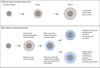 |
Fig. 1 Schematic overview of pre-runaway envelope accretion. When the solid material does not interact with the envelope, the gas accretion is initially determined by the size of the core and the strength of the accretion luminosity (Phase I). The core stops growing when there is no more solid material available, so the envelope accretion rate is determined by the cooling timescale of the protoplanet (Phase II). If Phase II is efficient, the planet can reach critical mass within the lifetime of the protoplanetary disk. It will go into runaway accretion and become a gas giant. Gas accretion from the nebula is different when the interaction of the solid material with the envelope is considered. Part of the ice and/or silicates will vaporize rather than reaching the core in solid form. This increases the envelope metallicity. The increased metallicity can, on the one hand, inhibit further gas accretion by increasing opacities in the envelope, which hinders cooling. On the other hand, the increased mean molecular weight increases the mean density of the envelope, which promotes gas accretion. |
Assumed initial solid surface density and initial gas surface density in the heavy, medium, and light disk.
2 Methods
The formation simulations are based on a modified version of the MESA code1 (Paxton et al. 2011, 2013, 2015, 2018, 2019), which was properly adapted to simulate planet formation and evolution (Valletta & Helled 2020; Müller et al. 2020a,b). The formation model is similar to the one used in Valletta & Helled (2020), with some modifications as discussed below.
The initial model has a core mass of 0.1 M⊕ and an envelope of 10−6 M⊕. The initial envelope metallicity is 0.03, but drops to zero at the beginning of the evolution when pure H-He is accreted and envelope enrichment is not yet significant. Three different solid accretion rate prescriptions are considered to compute the solid accretion rate ṀZ. Based on planetesimal accretion, we used rapid growth (Pollack et al. 1996) and oligarchic growth (Fortier et al. 2013). We also simulated pebble accretion (Lambrechts & Johansen 2014). A summary of these accretion rates are given in Appendix A. For planetesimals we assumed a radius of 100 km and for the pebbles one of 10 cm.
In the case of planetesimal accretion the simulation starts at 10 kyr. In the pebble accretion case we also assumed that the solid accretion rate starts at 10 kyr, but with a smaller initial model, namely 0.01 M⊕. Integrating the solid accretion rate of pebbles (see Appendix A.4) from a mass of 0.01 M⊕ at 10 kyr to 0.1 M⊕ gives us the starting times of our planetary embryo. These starting times (t0, peb) depend on the disk conditions and are given in Table 1.
In the nominal case we set the lifetime of the disk to 10 Myr. As solar-like stars should form within 5–10 Myr, this is a long but not unlikely formation time (Pfalzner et al. 2022). We also considered a shorter formation duration of 3 Myr. We stopped our simulations before runaway gas accretion started, namely when the crossover mass was reached, where the envelope and core are of equal mass (Bodenheimer & Pollack 1986; Pollack et al. 1996).
2.1 Boundary conditions and disk assumptions
The outer boundary conditions of our model planetary envelope (Pout and Tout) are set equal to the pressure and temperature in the disk. Following Piso & Youdin (2014) these are given by scaling relations in distance:
 (1)
(1)
 (2)
(2)
where a is the orbital distance of the protoplanet. The normalization factors that we applied are higher than the fiducial Minimum Mass Solar Nebula (which would be 0.0085 and 60 for pressure and temperature, respectively). While this is a significant increase, we find that it does not influence the envelope masses when they are above ~0.01 M⊕ and saves computation time. These boundary conditions do play a significant role in the early stages of the protoplanet and could in theory alter the formation path, for example through the onset of fragmentation. Similarly, Pout and Tout are assumed to remain constant in time in this work. More accurate gas accretion simulations would thus require an improved disk model, especially for the cases presented with envelope masses below 0.01 M⊕ after formation. In this work, however, these simplification suffice to demonstrate the importance of envelope enrichment on gas accretion.
The planetesimal accretion rates scale linearly with the solid surface density, ΣZ, at the location of formation (see Appendices A.1 and A.2). The initial solid surface density ΣZ,0 is given by
 (3)
(3)
The solid surface density decreases as solids gets accreted onto the planet.
The pebble accretion rate has a linear dependence on the gas surface density at 1 au, β (see Appendix A.4). β is set by an initial gas surface density β0 and decreases exponentially in time (t):
 (4)
(4)
where τdisk is the gas disk lifetime, which we fixed to 3 Myr. C1 and β0 are used as free parameters to account for disks of different masses. We set C1 to 5, 7.5, or 10 g cm−2 for a light, medium, or heavy disk, respectively. Values of β0 for these three disk types are set to 250, 500 or 750 g cm−2. The corresponding values of Σz,0 and Σ𝑔,0 at 3 or 5 au are listed in Table 1.
The inner boundary of the envelope model is the core. The luminosity at the core-envelope interface is determined by the accretion luminosity:
 (5)
(5)
where G is the gravitational constant and fabl is the fraction of solid material that is ablated or fragmented in the envelope. Mc and Rc are the core mass and radius, respectively, where the value of Rc is calculated assuming a constant core density of 3.2 g cm−3, regardless of the composition of the accreted material. The significance of this simplification is considered in Appendix C.
2.2 Enrichment from planetesimals or pebbles
The interaction between the accreted solids and the envelope is considered via the fragmentation and/or ablation of the solids (planetesimals or pebbles). The calculation of the value of fabl is given in Appendix B. This method also gives the deposition profile mdep (r) at radius r. The amount of water vapor added to the envelope is the product of fabl and the solid accretion rate.
We considered two deposition methods. The first was direct deposit. In this method the mass is deposited at the radial locations where ablation and fragmentation occur. For example: if a planetesimal fragments at radius r and there is no prior ablation, the water mass in layer m(r) is enhanced by the solid accretion rate. This increases the metallicity.
The second method, homogeneous deposit, is the default in this work. It assumes that the mass deposition is completely smoothed over the envelope, which has total mass Menv. This means that the amount of added heavy material is distributed over all layers, normalized to the layer’s mass, where
 (6)
(6)
As an illustration, Fig. 2 shows the difference between direct deposit and homogeneous deposit specifically for a planet growing by oligarchic growth at 5 au after 47 kyr. The core mass is still the initial 0.1 M⊕ and the envelope mass is 1.5 × 10⁻⁵ M⊕. The envelope is too small to cause fragmentation of the plan-etesimals and thus there is only ablation. The fraction of ablated material increases toward the interior of the envelope. The homogeneous deposit is completely smoothed over all layers, but the total deposited material adds up to the same as for direct deposit.
While at every timestep the deposition of heavy material is done homogeneously, this does not necessarily mean that the composition in the envelope is homogeneous. This is for two reasons. First of all because there is a gas accretion of pure H-He with zero metallicity added to the outer layers of the envelope. The inner layers, which are older, will have been exposed to envelope enrichment for longer and thus have a higher metallicity. This will create a compositional gradient unless the Ledoux criterium is met, in which case the convective region will become homogeneously mixed. Secondly, we considered a maximum metallicity in each layer, and if this was already reached there was no enrichment. An example of this is shown in Fig. 2. The orange solid line shows the deposit profile, while the dashed orange line shows the actual enrichment. The difference is due to some layers in the envelope already being saturated, or close to saturation, meaning it is not possible to deposit all the mass without condensation. There are two criteria that could limit the amount of water that can be deposited in a certain layer.
First, we checked the material state of H2O based on the temperature of the layer and from there calculated the maximum number density of water in layer r:
 (7)
(7)
P(r) and T(r) are the pressure and temperature at radius r. Tcrit is the critical temperature of 647.096 K. In the cases where the temperature is below 647 K, we applied the vapor-liquid phase boundary from Wagner & Pruß (2002) to calculate the saturation pressure of water Psat as follows:
 (8)
(8)
Here Pcrit is the critical pressure, 220.64 bar.  . The other variables are a1 = −7.85951783, a2 = 1.84408259, a3 = −11.7866497, a4 = 22.6807411, a5 = −15.9618719, a6 = 1 80122502.
If the temperature exceeded the supercritical temperature of water we imposed a limit to the water enhancement, Zmax. Supercritical water and H-He are expected to be highly miscible (Soubiran & Militzer 2015), suggesting that Zmax = 1. However, in our nominal model we set this value lower to 0.9 to ensure that we did not artificially create a loss of H–He. This would happen if too much H-He inside the envelope is replaced by water without a sufficiently high primordial gas accretion rate. We also wanted to investigate the significance of this miscibility and additionally considered this maximum metallicity to be to 0.5.
The second criterion for water deposition is that the deposited material can only be as massive as the shell in which it is deposited. As MESA uses mass coordinates, this criterion ensures that there is no Rayleigh–Taylor instability created through the deposition. While this an artificial limit, we argue that the deposited material we calculate in a certain layer using our 1D model underestimates the smoothing over different layers. Thus, allowing this smoothing of the water deposition profile should allow the 3D structure to be better represented.
When it was not possible to deposit part of the heavy material in the envelope, we transferred the leftover water mass to the core. Thus, the enrichment is only equal to the initial deposition if a layer is not yet saturated, as is demonstrated in Fig. 2. In this specific case, the critical temperature is exceeded in the inner 10% of envelope mass (q < 0.1) such that the maximum metallicity is much higher than for q > 0.1. Furthermore, the outer envelope (q > 0 4) contains newer gas that has not been exposed to as much enrichment, and hence the enrichment increases toward the outside of the envelope. If the envelope is not convective a compositional gradient can be created.
Finally, we defined the metallicity of the envelope at location r as
 (9)
(9)
The change in the envelope’s metallicity alters the opacities and the equation-of-state of the envelope. The total envelope’s metallicity is referred to as Zenv and is defined by the total water mass fraction in the envelope:
 (10)
(10)
The opacities are calculated by adding the molecular opacities from Freedman et al. (2014) and grain opacities from Alexander & Ferguson (1994), following Valencia et al. (2013). We used an equation of state that mixes water with hydrogen and helium, taken from Müller et al. (2020b, see their Appendix A for details).
Finally, the heavy element deposition in layer r has two influence on the energy. First of all accretion luminosity is added by
 (11)
(11)
with M(r) the cumulative mass at radius r.
Secondly the vaporization of water decreases the energy by (Pollack et al. 1986)
 (12)
(12)
where cp = 4.2 × 10⁷ (erg g−1 K−1) is the specific heat of water, E0 = 2.8 × 10¹⁰ (erg g−1) is the latent heat of vaporization and ∆T is the change of temperature to reach vaporization, which we set to 373 K assuming that the incoming pebble or planetesimal has a temperature of 0 K.
In our simulations we distinguish between four types of solid-envelope interactions, which are presented in Table 2. For simplicity, we neglected the thermal ablation or fragmentation of silicates and focus only on water. Therefore, Case-1 is a reference case without any solid-envelope interactions. All solid material directly reaches the core-envelope boundary and the envelope never increases in metallicity. We considered the other extreme in Case-2. We assumed that all the solid material is ice and can enrich the envelope.
With Case-1 and Case-2 the most extreme, we used Case-3 and Case-4 to investigate other aspects related to our fragmentation and ablation model. Case-3 is a hybrid between Case-1 and Case-2. Half of the solid material are icy planetesimals or pebbles, which can enrich the envelope. The other 50% of the solid accretion rate consists of rocky material that directly reaches the core and does not interact. Finally, in Case-4 we limited the maximum allowed metallicity, Zmax (see Eq. (7)), to 0.5 if the temperature exceeded the critical temperature. Figure 3 visualizes the effects of these cases on the planet’s interior and envelope.
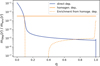 |
Fig. 2 Difference between the two deposit models: direct deposit (blue) and homogeneous deposit (orange). The x-axis gives the normalized mass coordinate of the envelope q. This figure specifically shows the deposit models for Oligarchic growth at 47 kyr when the envelope mass is 1.5 × 10⁻⁵ M⊕. There is no fragmentation yet. The ablation enriches the envelope metallicity up to 10% in the most inner region. The homogeneous deposit has the same total deposited mass, but smoothed. However, the actual enrichment is not homogeneous, as shown by the orange dashed line, due to some layers already being saturated. For different formation conditions and at different times the difference between the deposition and the actual enrichment changes. |
Solid-envelope interaction models considered in this work.
2.3 Gas accretion
Gas accretion can occur at every timestep. Following Valletta & Helled (2019), gas is added to the planet until the outer radius of the envelope is within a factor of 1.1 smaller or larger than the accretion radius. We used the accretion radius as in Lissauer et al. (2009). This formulation is based on the common assumption that the planet’s accretion radius must be equal to the smallest of either the Bondi radius or the Hill radius:
 (13)
(13)
where Mp is the mass of the protoplanet, cs is the speed of sound at the location of formation, RHill is the protoplanet’s Hill radius and k1 and k2 are reduction factors to account for the limited availability of gas at the formation location of the planet. For the small protoplanets considered in this study k1 and k2 can be set to 1.
The first 10 kyr are used to relax the envelope mass. The initial model does not automatically satisfy the criterion that the accretion radius equals the radius of the initial model. How much these two values deviate depends on the orbital distance. We smoothed this transition by finding k1 and k2 values such that the initial model radius is close to the accretion radius. Then we increased k1 and k2 linearly in time until these were both 1 at 20 kyr.
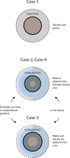 |
Fig. 3 Core and envelope compositions under the different solid-envelope interaction models presented in Table 2. The dashed black line represents the outer boundary to the envelope and the solid black line the inner boundary. Everything interior to the black solid line is considered as the core. The composition of the core and whether this is mixed is not considered in this work. Rather a constant core density of 3.2 g cm−3 is used. When envelope enrichment is considered this can either create a compositional gradient or there can (a) mixed convective zone(s), as shown by the two halves. |
3 Results
We performed a grid of simulations with the following variations: the solid accretion rate is rapid, oligarchic, or pebbles. The formation location is either 3 or 5 au and the disk is heavy, medium, or light, as defined in Table 1. An overview of all these results is given in Appendix D.
3.1 Solid-envelope interaction affecting H–He gas accretion
This subsection highlights the effect of all four solid-envelope interaction models on individual formation cases.
3.1.1 Rapid growth
Figure 4 shows the in situ formation of a planet by rapid growth at 3 au. The initial solid surface density is 17.33 g cm−2 (heavy disk). The upper panel shows the masses of the core (solid line) and envelope (dashed line) as time progresses for the various cases. We find that all the cases include both Phase I and Phase II of gas accretion, where the transition between them occurs after ~105 yr at a core mass between 4.4 and 5.2 M⊕. For Case-1 and Case-3, there is still a small increase in core mass during Phase II of gas accretion. At this stage, the planet grows through envelope accretion, which extends the planetary feeding zone and provides more solid material that can be accreted by the growing planet. In Case-2 and Case-4, on the other hand, the maximum core mass is reached, as any newly accreted planetesimals fragment and only add water vapor to the envelope. Another distinction is that Case-2 and Case-4 reach a crossover mass after 3.81 Myr and 2.5 Myr, respectively, while Case-1 and Case-3 do not reach crossover mass within 10 Myr. This is because in the first two cases the ablation-fragmentation transition occurs before the feeding zone is depleted and solid accretion is high. This promotes the gas accretion for several reasons. First, the total accretion luminosity is reduced, as a large fraction of the mass is deposited at larger radii and meanwhile the evaporation of water decreases energy locally. Second, the mean molecular weight of the envelope increases so that a more massive envelope can be bound. Similar to previous work we find that the increased opacities due to an increased envelope metallicity do not counteract the mechanisms promoting gas accretion. As such, envelope enrichment promotes total envelope accretion.
The lower panel of Fig. 4 shows the envelope’s growth, where the contributions of H-He are separated from the water vapor. Since Case-3 has a low-metallicity envelope, the total H-He mass in the envelope is similar to that of Case-1. We note that there would be a larger difference between Case-1 and Case-3 if fragmentation occurred before the solid accretion rate decreased. Case-2 and Case-4 have significantly more massive H-He envelopes at a given time. After ~105 years it remains a factor of 3 higher than Case-1 and Case-3. We find that for a short time the water mass in the envelope exceeds the H-He mass. This occurs during the transition between Phase I and Phase II. However, since subsequently mostly H-He is accreted, the envelopes final atmospheric composition is dominated by H–He.
During Phase II accretion, we find that small amounts of envelope mass can be lost. For Case-1 and Case-3, this concerns small oscillations in the envelope mass that are a result of an oscillating solid accretion rate. These are in turn due to the changes in capture radius, which depends on the internal structure of the envelope (see Appendix A.1). In other words, when the gas accretion rate is large, the capture radius also increases, promoting a higher solid accretion rate. However, the increase in luminosity from the gas accretion and the solid accretion expand the envelope and increase the radius beyond the accretion radius, which leads to mass loss. While the solid accretion rate remains small (between 10−8 M⊕ yr−1 and 0) this is sufficient to influence the envelope. Nonetheless, we do find that smoothing the change in capture radius during Phase II gas accretion (by only allowing it to change with 0.1% every timestep) eliminates these oscillations without altering the final outcome. In Case-2 we find a single instance of mass loss at 1.42 Myr. Similarly to Case-1 and Case-3 this mass loss proceeds from an increase in the capture radius. However, in this case the increased capture radius is due to a change in the internal structure of the envelope, as the size of the convective zone increases.
The top panel of Fig. 5 shows the envelope’s metallicity as a function of the total planetary mass. For all cases the envelope metallicity peaks when the feeding zone is depleted. The maximum envelope metallicity in Case-2 and Case-3 peaks at ~0.8. This is expected from the maximum metallicity in supercritical states, Zmax, set to 0.9. Colder outer layers where water can condense have even lower metallicities, which decreases the total envelope metallicity from zmax.
The lower panel of Fig. 5 shows H-He envelope mass as a function of the total planetary mass. Gray dashed lines give the reference fractions of fH−He = 0.1%, 1%, and 10%, where fH−He = Menv H−He/Mp. When the planet is smaller than ~2 M⊕ the primordial envelope masses of all cases are similar. At higher masses, the solid accretion rate increases and fragmentation occurs; as such, the envelope has a significant amount of water vapor, which influences the H-He accretion. At a total mass of 5 M⊕, Case-2 has a factor of 2 higher Menv, H−He than Case-1 and that of Case-4 is a factor of 5 higher than Case-1. However, at masses above 6 M⊕ the primordial envelope mass of Case-1, Case-2, and Case-4 converge, as Phase II of gas accretion sets in.
Interestingly, Case-3 has the transition into Phase II of gas accretion for a lower mass than the other three cases. Compared to Case-1, Case-3 has a lower core mass, as there is always a fraction between 0 and 0.5 of solid material evaporating in the envelope. Also, the maximum core mass is smaller compared to that of Case-2 or Case-4. This is because Case-2 and Case-4 are more efficient at enhancing the envelope and they reach a stage where fabl equals 1 before the feeding zone is depleted. As a result, envelope accretion accelerates and in this larger envelope planetesimals are captured more easily (i.e., the capture radius as defined in Appendix A.1 increases). Thus, as the solid accretion rate increases, the envelope becomes saturated with water vapor, which then allows the core to grow more rapidly as well. This acceleration of core and envelope formation is not evoked in Case-3 because of the later onset of fragmentation.
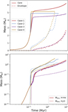 |
Fig. 4 In situ formation of a planet at 3 au with rapid growth. The simulations are run until the envelope and core are of equal mass or until 10 Myr. The initial solid surface density is 17.33 g cm−2 (heavy disk). The upper panels show the mass of the core and the mass of the envelope over time. The lower panel shows the same simulations as in the upper panel, but only the envelope masses over time. Solid lines are the mass from primordial H–He. The dashed lines are the envelope mass from water vapor. In Case-1 there is no water vapor as only hydrogen and helium are accreted from the nebula. |
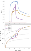 |
Fig. 5 Same simulations as presented in Fig. 4 but showing the heavy element fraction of the envelope (upper panel) and the primordial envelope mass, from pure H-He (lower panel). Both are shown as a function of the total mass (Mcore + Menv). The gray dashes lines indicate where primordial envelope mass fractions would be 0.1%, 1%, and 10% of the total mass. |
3.1.2 Oligarchic growth
Figures 6 and 7 demonstrate the effect of envelope enrichment on the planetary mass and bulk composition as well as the formation timescale for oligarchic growth at 3 au. Similar to the previously presented rapid growth, the initial solid surface density is 17.33 g cm−2, corresponding to a heavy disk.
The upper panel in Fig. 6 shows that in Case-2 the core reaches a maximum of 2.7 M⊕. This is notably lower than the core of the planet formed by rapid planetesimal accretion at the same location in a heavy disk. The reason for this difference is that the rapid formation has a high solid accretion rate with a large accretion luminosity. This makes the total envelope mass lower for a given core mass, and as such, complete fragmentation is reached for a higher core mass with rapid growth. However, the core mass presented in these results also contain evaporated water that could not be held in the saturated envelope layers. Further discussion on the impact of our core model assumptions on the accretion of H-He is presented in Appendix C. Case-4 has a larger core accretion rate than any of the other models in the last 3 Myr. This is because Case-4 has a more massive envelope and thus a larger capture radius. Furthermore, because zmax in Case-4 is lower than those in Case-2 and Case-3, the envelope becomes saturated earlier.
Since oligarchic growth is much slower compared to rapid growth, it takes longer before the core is massive enough to accrete an envelope with which the solids will interact. As shown in the lower panel of Fig. 6, the envelopes in Case-2 and Case-3 become water dominated after 2.7 and 1.8 Myr, respectively, and this composition persists during the remaining planetary growth. The H-He mass is unchanged for Case-1, Case-2, and Case-3 until 7 Myr, while Case-4 always has more H-He.
The upper panel in Fig. 7 confirms that the envelope metallicity increases at a smaller core mass for oligarchic growth compared to rapid growth. The maximum metallicities also occur at smaller core masses than for rapid growth because there is not enough time to grow larger cores. The lower panel shows that Case-1 and Case-2 have very similar H-He envelope fractions until Case-2 reaches its maximum core mass. Also, Case-3 and Case-4 have similar H-He envelope mass fractions. Overall, we find that the H-He mass fractions are larger in oligarchic growth than in rapid growth, since the envelopes for a given core mass are larger due to the slower formation.
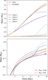 |
Fig. 6 Same as Fig. 4 but for a planet forming in situ at 3 AU via oligarchic growth in a heavy disk. |
3.1.3 Pebbles
Since pebble accretion is more efficient than planetesimal accretion, we find that most of our pebble simulations reach crossover mass before 3 Myr even when using a later starting time than for the planetesimal accretion. Only in the case of a light disk at 5 au we find planets in a pre-runaway state after 10 Myr. As a result, this is the formation scenario we highlight in Figs. 8 and 9. Due to the small size of pebbles, the value of fabl reaches 1 already at the beginning of the simulation. We used the first 3 kyr of the simulation to smooth fabl from 0 to 1 linearly in time.
Figure 8 shows that Case-1 and Case-3 do not reach a crossover mass while Case-2 and Case-3 reach it after 7.7 and 9.3 Myr, respectively. In Case-2 the maximum core mass is 3.9 M⊕ and for Case-4 it is 5.2 M⊕. Case-1 leads to a core mass of 6.3 M⊕ and an envelope of 0.88 M⊕ after 10 Myr while Case-3 ends with a 5.2 M⊕ core and an envelope of 2.6 M⊕.
There are instances of mass loss in Case-2 and Case-3. Contrary to the rapid cases, this is not linked to the coupling between the solid accretion rate and the envelope structure. Instead, this is due to the small size of the pebbles and their immediate fragmentation. In combination with our model setup, which allows the envelope to be considered “full” and adds additional water to the core, this can cause the value of fabl to drop when the metallicity is close to saturation. This allows temporary oscillations in the accretion luminosity and possibly, mass loss. These changes in fabl are unphysical and should be modeled more self-consistently in future work. It must be noted, however, that the interaction between icy pebbles and nebular gas can already enhance metallicities at distances further away from the protoplanet than where the gas is bound. In Sect. 5.3 we discuss this point and argue that this interaction needs to be well understood before it can be incorporated in 1D models.
The envelope’s metallicity and primordial envelope mass for the pebble cases are shown in Fig. 9. The metallicities peak at masses of 2–6 M⊕. We find that all the enrichment models follow roughly the same relation between the H-He mass fraction and the total mass, as shown in the lower figure. In comparison to the planetesimal accretion models in Figs. 5 and 7, however, these are less smooth. This is because the instant ablation of the pebbles.
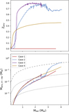 |
Fig. 7 Same as Fig. 5 but for a planet forming in situ growth at 3 AU via oligarchic growth in a heavy disk. |
3.2 H-He mass fractions after formation
Figure 10 summarizes all the nebular H-He mass fractions for the different formation scenarios presented in this work. This fraction is indicated by fH−He, which is the H-He mass in the envelope divided by the total mass of the planet. All panels show fH-He as a function of the total mass of the planet. Only masses below 15 M⊕ are shown to focus on mini-Neptune planets and because post-runaway gas accretion was not taken into account in our simulations. Planets that reached the crossover mass or had a total mass above 15 M⊕ were also removed from the figure. Dashed vertical lines reference where fH−He has values of 10%, 1%, and 0.1%.
The left panels show fH−He when the planet forms at 3 au. All the planetesimal cases (rapidandoligarchic)remainpre-runaway up to 10 Myr with the exception of Case-2 and Case-4 of rapid growth in a heavy disk. Rapid growth leads to larger masses and larger values for fH−He than oligarchic growth. This difference in composition between the two formation models is most visible at 3 Myr. If formation times are longer and there is strong envelope enrichment (Case-2) then oligarchic growth can create planets with total masses and H-He mass fractions that overlap those of rapid growth. Overall rapid growth can create planets of masses 2–9 M⊕ with H-He envelope fractions of 0.03–0.5 at 3 au. Oligarchic growth creates planets with total masses of 0.5–4 M⊕ with fH−He values of 5×10⁻⁴ to 0.1.
At 5 au there are not as many data points for rapid growth as the planets are likely to reach the crossover mass quickly. None of the heavy disk cases remain. The planet forming in a medium disk under Case-1 remains pre-runaway at 5 Myr and for Case-3 this is past 3 Myr. Planets forming by rapid growth with Case-2 can only do so in a light disk in 3 Myr. The oligarchic cases all remain pre-runaway and have smaller H-He mass fractions than at 3 au. This is because the planets forming at 5 au have smaller accretion radii due to a smaller Bondi radius. At some point the accretion radius becomes dominated by the Hill radius, which increases with distance. This will lead to planets at 5 au holding more massive envelopes than those at 3 au for the same total planetary mass. However, for the oligarchic growth cases, this transition happens too late to see reflected in H-He mass fractions at 3, 5, or 10 Myr.
Pebble accretion only forms mini-Neptune planets when there is a light disk, which is assumed to coincide with a late formation time (relative to a heavier disk). Furthermore, at 3 au a mini-Neptune can only form when Case-3 enrichment applies if formation lasts longer than 5 Myr. In Case-3 the total mass and fH−He stay within the same region as the planetesimal accretion models. Within 3 Myr a 13 M⊕ planet can also form by pebbles with so that fH−He=0.1 assuming Case-1 or Case-4. In Case-2 there are no pre-runaway planets even after 3 Myr.
At 5 au it is easier to form small planets by pebbles, although still exclusively for the light disk. This is contrary to planetesimal formation, which favors smaller planets at 3 au. After 3 Myr there is not yet a distinction between any of the enrichment models for pebble formation as they all lead to a planet of 2.5 M⊕ and a fH−He of 0.004. After 10 Myr only Case-1 and Case-3 have remained pre-runaway.
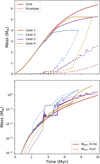 |
Fig. 8 In situ formation of a planet at 5 au by pebbles. The initial disk conditions are light. The upper left panel shows how the core mass and envelope grow in time. The lower left panel shows the envelope mass, with the separated mass contributions of H-He (solid lines) and H2O (dashed lines). |
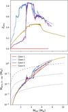 |
Fig. 9 Same simulations as shown in Fig. 8. Dashed gray lines show H-He envelope mass fractions of 0.1, 0.01, and 0.001. |
3.3 Envelope metallicities after formation
In Figs. 11 and 12, the maximum envelope metallicities (Zenv, max) are shown for the same set of models as in Fig. 10, with the exception of Case-1, which by definition evolves to a zero metallicity envelope. Horizontal lines indicate the maximum imposed metallicity for supercritical layers, Zmax.
For rapid growth, the maximum metallicity always occurs before 400 kyr, which is significantly quicker than the shortest considered formation time of 3 Myr. It is therefore unlikely that rapid growth at 3 or 5 au can create mini-Neptune planets with very high metallicity envelopes (that is, envelope metallicities that are close to Zmax).
On the other hand, during oligarchic growth, maximum metallicities occur very late, between 4.6 and 10 Myr. They correspond to total masses of 0.5 to 3 M⊕. The oligarchic cases never reach saturation where the envelope metallicity is that of Zmax.
The pebble cases show a wider spread in times when Zenv, max is reached. For most of the pebble cases, we find that the maximum metallicity occurs before 3 Myr, but could be delayed to 4 Myr or even 7 Myr if the disk is light.
4 Discussion
4.1 The effect of mixing and the location of deposits
The results presented above assumed a homogeneous composition of the envelope due to convective mixing at layers where the Ledoux criterium is met. While it is expected that there is some mixing in protoplanetary envelopes, it is unclear how efficient mixing is. Simulating the planetary formation with MESA allows mixing to be included via the mixing length theory (mlt). This, however, requires the knowledge of a dimensionless parameter αmlt (see Sect. 2.4 in Valletta & Helled 2020). For the formation of Jupiter Valletta & Helled (2020) adapted αmlt = 0.1 (Vazan et al. 2015; Müller et al. 2020b) and we use the same mixing in our nominal model. In this subsection we investigate the effect of mixing by considering a model in which mixing is inhibited.
The effect of mixing on the protoplanets core and envelope mass and composition are shown in Fig. 13 for the oligarchic growth at 3 au for Case-2. The initial solid supply is heavy. When mixing is included this increases the efficiency of the deposit of heavy elements. The mixing distributes the H-He through the envelope such that there are more layers where the maximum metallicity is not met. This allows for a larger overall deposit of heavy elements. As a consequence the mixing model reaches a point where fabl reaches 1 after 7 Myr. The accretion luminosity becomes zero and gas accretion increases. The final H-He envelop mass is an order of magnitude larger and the core mass is 0.5 M⊕ smaller.
We also investigate the effect of our assumption of a homogeneous deposition of heavy elements in the envelope. We compare the homogeneous deposit to the direct deposit as defined in Sect. 2.2.
Figure 14 shows the differences between these deposit models for Rapid growth at 3 au, Case-2. The nominal, homogeneous deposit is the same as shown in Fig. 4. In the case of direct deposit, is takes longer for the envelope to start growing significantly. This is because initially only ablation occurs, which means that in the direct deposit case there are only heavy elements in the lower layers. In the homogeneous deposit case, water is added to the outer layers as well, so the density increases and that causes fragmentation to occur more quickly (see Eqs. (B.4) and (B.5)). Due to this fragmentation almost no solids reach the core so that the accretion luminosity from solid accretion decreases and gas accretion increases. The model with a direct deposit of solids reaches fragmentation later. Nevertheless, when both models have reached fragmentation the gas accretion is more efficient in the direct deposit. In that case the mass can be deposited high in the envelope and “trickle down” to the lower layers. The crossover mass is then reached after 1.39 Myr instead of 3.81 Myr.
A realistic deposition profile of heavy elements should lie somewhere in between the two extreme cases that we considered in this work. Assessing the physical importance of mixing on planet formation, in combination with envelope enrichment, would require the following improvements. First, the 1D deposit profile needs to be smoothed appropriately to account for the 3D process (Mordasini et al. 2017). In the case of planetesimal accretion this initial deposit profile would also need to be improved upon by using a more realistic size distribution (Kaufmann & Alibert 2023). Second, the treatment of envelope metallicity should be improved. In this work, the accreted heavy-element mass was added by increasing the metallicity and changing the energy in the relevant layers. However, mass in every layer was conserved during enrichment. Future work should treat mass deposition and envelope enrichment self-consistently by allowing this process to directly change the mass of the relevant layers.
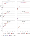 |
Fig. 10 H-He mass fraction after 3 Myr (upper panels), 5 Myr (middle panels), and 10 Myr (lower panels). The left panels show in situ formation at 3 au and the right panels at 5 au. The colors indicate the heavy-element interaction models. Case-1, Case-2, Case-3, and Case-4 are given in red, blue, purple, and yellow, respectively. The three different solid accretion rates are distinguished by different symbols. We also show the light initial disk results by a transparent marker, the medium disk result with a 0.5 opacity marker, and the heavy disk result with a full opacity marker. The light, medium and heavy results of the same model are connected by a line, as we would expect that in intermediate disk would produce a final H-He fraction approximately along this line. The total masses in the figure are limited to below 15 M⊕, focusing on the distribution for mini-Neptune type planets. Planets that reached the crossover mass (Menv = Mcore) are not shown, even if their total mass is below 15 M⊕. |
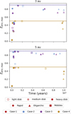 |
Fig. 11 Maximum envelope metallicity that is reached during planetary formation (Zenv, max) and the time at which this maximum metallicity occurs. The horizontal lines indicate the imposed maximum metallicity for supercritical water (Zmax in Table 2). |
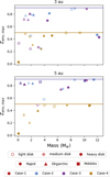 |
Fig. 12 Same data as in Fig. 11 but instead of the time, the total mass of the protoplanet is shown when the maximum envelope metallicity is reached. |
4.2 Primordial envelopes and habitability
Planets with a primordial, H-He dominated envelope have received increased attention as potentially habitable candidates. The collision-induced absorption of hydrogen can act as a greenhouse effect and thereby create temperate surface conditions (Stevenson 1982; Pierrehumbert & Gaidos 2011; Madhusudhan et al. 2021; Mol Lous et al. 2022). Madhusudhan et al. (2021) coined the term “Hycean planets”, which host liquid water underneath a hydrogen-dominated atmosphere. It remains uncertain, however, whether any of the currently observed transiting exoplanets orbit in what can be considered the “Hycean habitable zone”. The role of a runaway greenhouse effect (Pierrehumbert 2023; Innes et al. 2023) and atmospheric escape (Wordsworth 2012; Mol Lous et al. 2022) could move the inner habitable zone boundary in comparison to an Earth-like planet.
Another open question regarding Hycean planets is whether such planets can accrete the required amount of H–He to enable these temperate surface conditions in the first place. In Mol Lous et al. (2022), we showed that planets of sizes 1–10 M⊕ that orbit around a Sun-like star could host temperate conditions if they are beyond 2 au. Their primordial, pure H-He envelope could have masses of 10−4-10−5 M⊕ at this distance, but more massive when farther out. The results presented in Fig. 10 show that H-He envelope below 10−3 are generally difficult to form, and most of the formed planets consist of much larger H-He mass fractions. The smallest H-He envelopes are formed by oligarchic growth at 5 au. After 3 Myr, these planets have values for Menv, H-He ranging from 2.7 ×10⁻⁵ M⊕ (fH−He = 10−4 when the total mass is 0.27 M⊕) up to 2.24 ×10⁻⁴ M⊕ (fH−He = 4 × 10⁻⁴ when the total mass is 0.56 M⊕). These planets are smaller than those considered in Mol Lous et al. (2022), but still massive enough to hold onto a H-He envelope at 5 au (Mordasini 2020). We therefore conclude that the formation of H-He envelopes that provide temperature surface conditions is probably rare but possible when the planet forms beyond the ice line and the formation timescale is long.
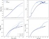 |
Fig. 13 Oligarchic growth at 3 au in a heavy disk. The light blue line indicates Case-2 without mixing and the dark blue line is for the same conditions but with mixing (αmlt = 0.1). When mixing is included, it distributes the H–He through the envelope. As our method replaces H-He with water, mixing increases the efficiency of water deposition. As a result, in the mixing cases there are cases where all the water can be deposited in the envelope. This reduces the accretion luminosity, which leads to acceleration of the envelope’s growth. |
5 Caveats
5.1 Envelope-core interactions and outgassing
Our model does not include interactions between the envelope and the core. We assume that all the nebular hydrogen and helium remain in the envelope and that none is sequestered in the core, to be outgassed at later stages. For (super-)Earth this can play an important role in the development of the atmosphere after the gas disk has disappeared (Elkins-Tanton & Seager 2008; Schaefer & Fegley 2010). As silicates in the core are expected to be in the magma phase there should be a high solubility of hydrogen (Hirschmann et al. 2012). That hydrogen would over time be outgassed and replenish the envelope (Chachan & Stevenson 2018), but that would be accompanied with the atmospheric escape of mostly hydrogen. There could also be a later increase in atmospheric hydrogen if metal-rich impactors oxidate (Genda et al. 2017). Thus, some of the H-He mass calculated in this work could be stored in the core and released gradually.
The envelope–core interactions for H2O, not considered in this work, should also be mentioned. While we focus on predicting the mass fraction of H-He after disk accretion, the treatment of water can be improved, which could lead to different results. Water can also be stored efficiently in a magma ocean and out-gassed later (e.g., Dorn & Lichtenberg 2021; Bower et al. 2022; Sossi et al. 2023), which can increase the envelope’s metallicity after formation.
5.2 Ablation and fragmentation of silicates
In this work, we only modeled the effect of water enhancement on the envelope. It is clear that rocky material can also ablate and fragment. This is especially the case for pebbles (Brouwers et al. 2018; Brouwers & Ormel 2020; Steinmeyer et al. 2023), but also for planetesimals (e.g., Bodenheimer et al. 2018). Similar to water enrichment, the enrichment with silicates on the one hand increases the mean molecular weight and promotes gas accretion and on the other hand enhances the opacities in the envelope (Ormel 2014; Mordasini 2014; Menou & Zhang 2023). The enrichment of silicates alone can create a composition gradient that inhibits convection (Ormel et al. 2021; Markham et al. 2022). This silicate enrichment has an effect on the long-term evolution of mini-Neptunes and not considering this effect can lead to over-predictions of H-He mass fractions in observed planets (Misener & Schlichting 2022; Vazan & Ormel 2023).
Future work should consider the enrichment of both water and silicates in the envelopes of protoplanets. However, accounting for both species will introduce more free parameters concerning the mixture of ice and silicates in the solid accretion rate.
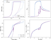 |
Fig. 14 Rapid growth at 3 au in a heavy disk. The light blue line shows a homogeneous deposit of heavy elements, which is the default in our model. The purple line shows how the results change when the heavy elements are directly deposited at the relevant radial distance in the envelope. |
5.3 Limitations of a 1D model
The assumption of spherically symmetric gas and solid accretion that comes with a 1D model does not accurately reflect the reality and thus there are some limitations. First of all there is the recycling of gas that occurs in the outer regions of the accreting envelope. The nebular gas from the disk has a higher entropy than the already accreted gas in the envelope and will mix (Ormel et al. 2015). This will delay the cooling and contraction, thus prolonging Phase II of gas accretion. Recycling is an important aspect of planet formation. It can significantly delay the formation timescale, which can help explain the presence of super-Earths and mini-Neptunes, when 1D models would have predicted a transition into runaway gas accretion. This could also possibly help with the formation of Uranus and Neptune (Eriksson et al. 2023). Three-dimensional gas accretion simulations remain computationally expensive. Recently Bailey & Zhu (2023) found a more optimistic comparison between 3D and 1D models. They suggest that 1D models can improve their accuracy by reducing the accretion radius to 0.4 times the Bondi radius and considering two distinct outer recycling layers.
A second limitation revolves around the deposition profile of heavy elements. In this work we have considered two extremes. In the nominal case we deposited the heavy elements homogeneously. Alternatively, we solved the deposition profile in the 1D case and deposited the solids accordingly. The latter is realistic if the solid accretion rate is isentropic and the timescales of the impacts is shorter than the azimuthal mixing (Mordasini et al. 2017).
5.4 In situ formation
The effect of migration is neglected in this work although in situ formation is rather unrealistic. One origin theory of mini-Neptunes is that they form around the ice line and migrate inward once they reach a critical mass (Kuchner 2003; Venturini et al. 2020; Huang & Ormel 2022; Burn et al. 2024). The precise value of this critical mass remains uncertain (McNally et al. 2019; Paardekooper et al. 2023) though derivations of it can be found, such as in Emsenhuber et al. (2023). This formation scenario would naturally lead to a diversity in mini-Neptunes (Bean et al. 2021).
In the rapid growth case, some planets in our simulations deplete their feeding zone and enter Phase II gas accretion. We predict that if migration is included this will lead to larger planets. However, our conclusion that different treatments of solid-envelope interactions can heavily influence the outcome of planet formation is robust.
6 Summary and conclusions
We simulated planet formation assuming different solid accretion rates, and calculated the corresponding gas accretion rate self-consistently. The planetary formation locations were set to be outside of the ice line, where the observed mini-Neptunes could have formed before migrating to shorter orbital distances. Our study clearly shows that the assumptions used by planet formation models play a key role in determining the planetary growth history and therefore also the planetary mass and composition. Our key conclusions can be summarized as follows:
The assumptions regarding the interaction between solids and the planetary envelope strongly affect planetary growth and can change the primordial gas mass fraction by up to a factor of 10. Nevertheless, we have also identified cases where this interaction has little to no influence on the forming planet. In the case of oligarchic growth, the envelope remains small and, despite being metal-rich, does not alter the rest of the formation process;
Forming mini-Neptunes at 3 au is challenging with pebble accretion due to the high accretion rates. Their formation via pebble accretion becomes more likely at 5 au, when the initial disk is relatively light. However, we place more caveats on our pebble result compared to the planetesimals because (1) pebble growth strongly depends on the start time of the growth, and (2) pebbles could sublimate before reaching the accretion radius, which might influence the results;
The impact of envelope pollution is complex. The most extreme solid-envelope interaction cases (Case-1 and Case-2) do not automatically lead to the most extreme outcomes. On the contrary, we find that our Case-4, in which half of the solids interact, does not necessarily lead to planets in between the more extreme cases. For example, with rapid growth at 5 au, we find that Case-4 leads to the smallest planets for a given time;
Envelopes of protoplanets during Phases I and II of gas accretion can be dominated by heavy elements;
Our results are consistent with the observed diversity of exoplanets (e.g., Jontof-Hutter 2019). Variations in the formation location, the solid material in the protoplanetary disk, the composition of the solid material, and the formation timescale determine the final mass and composition of the forming planets. We find that fabl can span a range of several orders of magnitude and that the envelope’s metallicity can range from 0 to full saturation. Our results clearly imply that low- to intermediate-mass planets should be diverse in terms of mass and composition, depending on the exact formation conditions and growth history.
We find that including envelope-solid interactions in gas accretion models can significantly influence planet formation even for low planetary masses. This has an important impact on our understanding of the formation of mini-Neptunes. We note that assuming pebble or planetesimal accretion exclusively could lead to an overestimation of cases that enter runaway gas accretion. Kessler & Alibert (2023) show that giant planet formation can be suppressed when both pebbles and planetesimals are considered.
Although the topic is still being investigated, it is often assumed that observed mini-Neptunes and super-Earths have a large water mass fraction (Venturini et al. 2020; Luque & Pallé 2022). This is further supported by the observation of volatile-rich planets in, for example, Kepler 138-c and Kepler 138-d (Piaulet et al. 2023). Furthermore, there are observations indicating the presence of atmospheric water vapor (e.g., Mikal-Evans et al. 2023). However, detecting atmospheric water is challenging due to the possible formation of clouds. Water signatures can also overlap with those of methane (Bézard et al. 2022). For K2-18b, which became famous as the first mini-Neptune detected with water vapor in its atmosphere (Benneke et al. 2019), JWST data have confirmed that the measured signature was due to methane, and not water (Madhusudhan et al. 2023). For highly radiated planets, JWST should be able to better constrain the volatile abundances (Acuña et al. 2023; Piette et al. 2023). If future observations can confirm that mini-Neptunes and super-Earths have water-rich atmospheres, this would support the idea that they formed beyond the ice line and migrated inward, as we assumed here. Other explanations for water-rich atmospheres of small planets could be a late volatile delivery (Elkins-Tanton & Seager 2008) or in situ water formation (Kite & Schaefer 2021).
Our results demonstrate that primordial gas accretion rates are not simple. Assumptions regarding solid-envelope interactions, the solid accretion rate, and the formation location can greatly influence the fraction of H-He after formation. These assumptions as well as aspects not considered in this work (migration and grain opacities) will need to be considered to explain the observed mini-Neptune and super-Earth population.
Acknowledgements
We thank Simon Müller for contributing to the re-writing of the original code used in Valletta & Helled (2020) and for helpful discussions. We also thank the referee for their valuable comments. This work has been carried out within the framework of the National Centre of Competence in Research PlanetS supported by the Swiss National Science Foundation under grants 51NF40_182901 and 51NF40_205606. The authors acknowledge the financial support of the SNSF.
Appendix A Overview of solid accretion rates
Appendix A.1 Rapid growth
Here we give an overview of how the solid accretion rates were calculated. In the case of rapid growth we calculate the solid accretion rate, ṀZ, from Pollack et al. (1996), Eq. 1:
 (A.1)
(A.1)
which uses the gravitational focusing factor Fg. This is calculated following Greenzweig & Lissauer (1992) (analytical approximation from Appendix B). Ωk is the orbital frequency. ΣZ is the solid surface density, described in A.3).
The capture radius (Rcap, or “enhance radius”) is calculated as in Inaba & Ikoma (2003), by considering the drag of the already accreted envelope. Using the assumed radius (rpl) and density (ρpl) of the planetesimals, we find the capture radius Rc in the envelope where it holds that
 (A.2)
(A.2)
which also uses the Hill radius of the protoplanet (RHill). When there is no sufficient envelope accreted, the capture radius is reduced to the core radius.
Appendix A.2 Oligarchic growth
Oligarchic growth is based on the idea that the planetary embryo can already be massive enough to perturb the planetesimals, increasing the temperature and reducing the solid accretion (Ida & Makino 1993). It leads to much longer formation timescales than rapid growth. We adapted the accretion rate from Fortier et al. (2007, Eg. 10):
 (A.3)
(A.3)
where F is an efficiency factor that needs to compensate the fact that the accretion rate is underestimated when the planetesimals are assumed to have eccentricities and inclinations all equal to the rms. In Greenzweig & Lissauer (1992) it is estimated to be ≈ 3. Following Fortier et al. (2007) we approximate the inclinations and eccentricities as
 (A.4)
(A.4)
and find e using Equation 10 from Thommes et al. (2003).
Appendix A.3 Solid surface density
The initial solid surface density, ΣZ,0, is calculated by Equation 3. The planet accretes solid materials from its feeding zone. The extend of this zone reaches  in both the inner and outer direction, following Pollack et al. (1996). Therefore, the inner and outer radii of the feeding zone are given by
 (A.5)
(A.5)
 (A.6)
(A.6)
where e is the planetesimal’s eccentricity. In the case of rapid growth this is calculated by Equation 6 in Pollack et al. (1996).
While the solid surface density is expected to be lower at Rin and higher at Rout compared to ΣZ,0, this will partly cancel out such that the difference is negligible. The ΣZ reduces when solid material is accreted onto the planet. We calculated ΣZ as
 (A.7)
(A.7)
with Macc being the already accreted solid material. Not considered are the scattering of planetesimals by the growing proto-planet (Zhou et al. 2007; Shiraishi & Ida 2008), which would decrease the amount of solid material.
Appendix A.4 Pebble accretion
The solid accretion rate of pebbles is adapted from Lambrechts & Johansen (2014), Eq. 31. It is given by
 (A.8)
(A.8)
where Z0 is the disk’s metallicity and it is set to 0.010270. β is given in Equation 4 and τdisk = 3 × 10⁶ yrs.
Furthermore, there is a multiplication with a 3D factor from Venturini & Helled (2017), which slightly reduces the mass accretion rate. This 3D factor is
 (A.9)
(A.9)
with  . is the disk’s viscosity, which is set to α = 10−4. Hgas is the scale-height of the gas disk Hgas = cs/Ω. This is approximated as (h = H/r) with h(r) = h0(r/AU)1/4. In the standard case, h0 = 0·036 (see Section 2.2 of Venturini & Helled 2017) Finally, Equation 20 of Lambrechts & Johansen (2014) is
 (A.10)
where we use ϵp=0.5 and η = 0·0015 × (a/1 au). Pebble accretion stops when the pebble isolation mass (Miso) is reached. Based on (Lambrechts et al. 2014), we used
 (A.11)
It is believed that the pebble accretion abruptly halts once the isolation mass is reached. In this work, however, we smooth the transition by applying a reduction factor to the pebble accretion rate. This reduction factor is 1 until the total mass is above half the isolation mass and linearly reduces in mass; therefore, it is 0 when the total mass equals the pebble isolation mass.
Appendix B Fraction of ablation
The fraction of ablating or fragmenting material (fabl) is calculated every timestep and changes as the size and composition of the envelope change. We follow the semi-analytical approached derived in Valletta & Helled (2019), which was based on the mass loss and motion of a planetary envelope derived in Podolak et al. (1988). The interacting solid material is assumed to be water. Therefore, the density of the planetesimals or pebbles is set to be ρpl = 1 g cm−3. This is similar to previous assumptions (Venturini et al. 2016; Valletta & Helled 2020) that are justified by observation of comets that indicate that water is the mayor volatile specie in the solar-system. Of course in reality, the accreted material is unlikely to be made of pure water. Below we refer to the impactors as planetesimals although the same method is applied for pebbles.
We integrate the planetesimals’ position, mass, and velocity from the outer boundary of the envelope model to the inner boundary, or until all the planetesimal mass is ablated or fragmented. The assumed initial velocity and location are υinit =10 km sec−1 and rinit = 2Rpl, respectively, with Rpl being the outer boundary of our model. The planetesimal’s velocity at location r inside the envelope is given by
 (B.1)
(B.1)
Weneglectedtheenvelope’s mass beyond the location r since the mass is negligible compared to the core mass and lower part of the envelope. The mass loss at location r is calculated using Equation 14 from Valletta & Helled (2019):
 (B.2)
(B.2)
where mpl is the mass of the planetesimal, A is the area of the planetesimal, which naturally decreases as the planetesimal loses mass, and ρ(r) is the density at r. Ch and ϵ are efficiency factors for which the appropriate values are uncertain. Ch is the fraction of kinetic energy transferred to the planetesimal. ϵ is the product of the emissivity of the gas and the planetesimal’s impact coefficient. We set both to 0.01. In Valletta & Helled (2019), Ch and ϵ were left as free parameters and while their value affects planetary growth, its effect is smaller in comparison to other assumptions considered in this work, such as the solid accretion rate and envelope mixing. Unlike in Valletta & Helled (2019), here we simplify the calculation of the planetesimal’s trajectory by assuming that it moves straight to the core. In other words, we assume an impact parameter of 0 and no angular contributions to the velocity. Q is the latent heat caused upon vaporization and is given by
 (B.3)
(B.3)
Here Cp is the specific heat of water in the liquid phase, set to 4.2×10⁷ erg g−1 K−1. E0 = 2.8 × 10¹⁰ erg g−1 is the latent heat of vaporization in the solid phase. The values are taken from Pollack et al. (1986) (Table 1). Tf is the difference between the initial temperature and the present temperature, which is 373 Kelvin.
The planetesimal can be completely destroyed when two conditions are met (Pollack et al. 1986). First, if the pressure gradient in the envelope surrounding the planetesimal is larger than the material strength:
 (B.4)
(B.4)
with S being the strength of the compressive material, set to 1 × 10⁶ Ba (0.1 Mpa) for ice (Pollack et al. 1979). Second, if the planetesimal is sufficiently small so that its self-gravity cannot prevent fragmentation:
 (B.5)
(B.5)
If both of these criteria are met, fragmentation occurs and fabl is set to 1.
Appendix C Importance of the core’s mass-radius (M-R) relation
In our current model the changes in the core’s composition are not considered. All the material that reaches the core, whether that is ice or solids, adds to the core mass in the same way. Using the total accreted mass and assuming a constant core density of 3.2 g cm−3 we calculate the core radius and this core radius sets the lower boundary in our atmosphere model. A more realistic model would need to infer the core’s radius with an interior model based on the assumed accreted material. We evaluate the influence of the core density on our results by using a gradually decreasing or increasing core density.
We do not consider the interaction of rocky material, and for simplicity the rock fraction in the core follows directly from the solid accretion rate. The water/ice mass fraction can have two different sources. First, it was directly accreted, which happens when there is no fragmentation. Second, there could be water excess since not all the water could be deposited in the envelope. We also consider this to be part of the core although in reality this should be added to the envelope mass at the lower layers, creating an ocean.
The upper panel in Figure C.1 shows the core’s composition for oligarchic growth at 3 au with Case-2. From the assumption that in Case-2 there is no rock in the solid accretion rate, the rock fraction of the core only decreases. The lower panel shows the core composition for Case-3, which by definition always has at least 50% accreted rock directly onto the core. The dark blue represents ice that is directly accreted to the core. The light blue is also water added to the core, but water that did not fit in the envelope and was thus moved to lower layers. For both of these water contributions to the core it is unknown what their thermo-dynamic properties would be. While the directly accreted water would reach the core in the solid phase, a subsequent impact might still vaporize, therefore also adding water vapor to the envelope. Some water did not fit in the envelope because the outer layers were too cold for water vapor (small envelope) and the water thus condensed. It is more common that all layers have reached the maximum metallicity for supercritical water. Figure C.2 shows the M-R relation of the core with a constant density of 3.2 g cm−3. For comparison, we also show the mass-radius relationships of planets taken from Zeng et al. (2019). These M-R relations are for planets including their atmospheres and should thus not be directly compared to the M-R of the core. Regardless, we applied another core density subscription based on a pure rocky planet, as our aim is merely to determine whether the core’s radius can affect the results of our formation model. We find that scaling the core density as  gives a similar core radius to the 100% rock planet (see “Increasing ρ” in Figure C.2).
Changing the core’s density has two competing effects. On one hand, a higher core density leads to a smaller core radius and this core radius is used as a lower boundary in the atmosphere model. Meanwhile, the accretion radius stays the same, so the volume that the envelope occupies is slightly larger and the envelope can be more massive. This effect, however, is very small since the core radius is about two orders of magnitude smaller than the accretion radius. On the other hand, a higher core density increases the accretion luminosity, which decreases the amount of gas that can fit within the accretion radius.
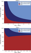 |
Fig. C.1 Core composition during oligarchic growth at 3 au with a heavy initial disk. The upper panel shows Case-2, where only water is accreted. As a result, the rock mass fraction, which is the initial model, decreases. The lower panel shows Case-3, where 50% water and 50% rock is accreted. As all the rock directly reaches the core, but the water can evaporate in the envelop, the core always has a rock mass fraction above 50%. The water that is added to the core can either directly reach the core (dark blue regions) or be added because the envelope was saturated (light blue). |
We applied this increasing core density to the formation with oligarchic growth at 3 au in Case-1, as this is the case that assumes the solid accretion is pure rock. The final envelope is indeed negligibly larger when using the higher density core, namely 0.082 M⊕ rather than 0.079 M⊕.
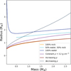 |
Fig. C.2 Mass-radius relationships taken from Zeng et al. (2019), shown with orange, light blue, and dark blue lines, are (a) 100% made of rock with an Earth-like composition (i.e., 32.5% iron and 67.5% MgSiO3) (b) 50% made of an Earth-like rocky core and 50 or (c) 100% pure H2O. The purple line shows the M-R relationship for a constant density of 3.2 g cm−3, the default used in this work. The increasing ρ model is a fit to the rocky core composition. The decreasing ρ is the minimum decrease in core density that affects the gas accretion rate. Since the gas accretion rate is only altered when the core’s density is significantly lower than interior models predict, we conclude that our assumption of a constant core density does not significantly influence the results. |
We do a similar study for the water-rich core in Case-2 but using an arbitrary scaling to the core’s density. Rather than trying to simulate the core’s M-R realistically, we simply decrease the density until we see a significant effect in our results. This is achieved when we decrease the density as ρc = 3.4 - 2(Mc/M⊕)1/3. As shown in the Figure C.2 this leads to core radii that are more than 1 R⊕ larger than pure water planets. Applying such a low core density to the oligarchic formation at 3 au with Case-2 leads to a core mass of 3.45 M⊕ rather than 2.71 M⊕ and an envelope of 0.3 M⊕ instead of 1.36 M⊕. The primordial envelope mass, Menv, H−He also decreases from 0.43 M⊕ to 0.07 M⊕. This occurs because a low density core eventually leads to a slightly smaller envelope and the fraction of ablation always remains low because there is not enough envelope to replace as water. However, the nominal core density model with a slightly larger envelope does reach a point where most of the solids can enrich the envelope and this causes a great reduction in the accretion luminosity, promoting gas accretion for the final 3 Myrs.
The core’s mean density that we have applied to a water-dominated core is notably lower than interior models predict (see Figure C.2 and, e.g., Haldemann et al. 2020). We therefore conclude that an extremely low core density can lead to significantly different primordial envelopes. However, we note that our variations in the core’s density is merely a parameter study and is not based on realistic interior models. A more realistic core model could be implemented in future work, where it would also need to be considered that rock and water would be mixed in this core (e.g., Vazan et al. 2022). At the same time, it should be noted that the core’s M-R relationship is likely to be less important in comparison to the effect of the chemical interactions between the core and envelope (see Sect. 5.1). This would play an important role in determining how the primordial gas is distributed within the planet.
Appendix D Result tables
Tables D.1, D.2, and D.3 give the composition of the (proto)planet when assuming rapid, oligarchic, and pebble growth, respectively. The core mass (Mcore), core water mass fraction (Xwater), envelope mass (Menv) and envelope metallicity (Zenv) are given at 3 Myr and 10 Myr. If the crossover mass is reached before 3 Myr, then the planetary composition at the crossover mass is given, rather than at 3 Myr, and no data are given for 10 Myr. If the crossover mass is reached between 3 and 10 Myr, the composition at the crossover mass is given rather than the composition at 10 Myr. The value of xwater strongly depends on the assumed solid accretion type, as discussed in Appendix C.
References
- Acuña, L., Deleuil, M., & Mousis, O. 2023, A&A, 677, A14 [NASA ADS] [CrossRef] [EDP Sciences] [Google Scholar]
- Alexander, D. R., & Ferguson, J. W. 1994, ApJ, 437, 879 [NASA ADS] [CrossRef] [Google Scholar]
- Alibert, Y. 2017, A&A, 606, A69 [NASA ADS] [CrossRef] [EDP Sciences] [Google Scholar]
- Alibert, Y., Mordasini, C., Benz, W., & Winisdoerffer, C. 2005, A&A, 434, 343 [NASA ADS] [CrossRef] [EDP Sciences] [Google Scholar]
- Bailey, A., & Zhu, Z. 2023, arXive-prints [arXiv:2310.03117] [Google Scholar]
- Bean, J. L., Raymond, S. N., & Owen, J. E. 2021, J. Geophys. Res. Planets, 126, e06639 [NASA ADS] [CrossRef] [Google Scholar]
- Benneke, B., Wong, I., Piaulet, C., et al. 2019, ApJ, 887, L14 [Google Scholar]
- Bézard, B., Charnay, B., & Blain, D. 2022, Nat. Astron., 6, 537 [CrossRef] [Google Scholar]
- Bodenheimer, P., & Pollack, J. B. 1986, Icarus, 67, 391 [Google Scholar]
- Bodenheimer, P., Stevenson, D. J., Lissauer, J. J., & D’Angelo, G. 2018, ApJ, 868, 138 [NASA ADS] [CrossRef] [Google Scholar]
- Bower, D. J., Hakim, K., Sossi, P. A., & Sanan, P. 2022, Planet. Sci. J., 3, 93 [NASA ADS] [CrossRef] [Google Scholar]
- Brouwers, M. G., & Ormel, C. W. 2020, A&A, 634, A15 [Google Scholar]
- Brouwers, M. G., Vazan, A., & Ormel, C. W. 2018, A&A, 611, A65 [NASA ADS] [CrossRef] [EDP Sciences] [Google Scholar]
- Burn, R., Mordasini, C., Mishra, L., et al. 2024, Nat. Astron., submitted [arXiv:2401.04380] [Google Scholar]
- Chachan, Y., & Stevenson, D. J. 2018, ApJ, 854, 21 [NASA ADS] [CrossRef] [Google Scholar]
- Chambers, J. 2017, ApJ, 849, 30 [NASA ADS] [CrossRef] [Google Scholar]
- Cimerman, N. P., Kuiper, R., & Ormel, C. W. 2017, MNRAS, 471, 4662 [Google Scholar]
- Denman, T. R., Leinhardt, Z. M., Carter, P. J., & Mordasini, C. 2020, MNRAS, 496, 1166 [NASA ADS] [CrossRef] [Google Scholar]
- Dorn, C., & Lichtenberg, T. 2021, ApJ, 922, L4 [NASA ADS] [CrossRef] [Google Scholar]
- Dorn, C., Khan, A., Heng, K., et al. 2015, A&A, 577, A83 [NASA ADS] [CrossRef] [EDP Sciences] [Google Scholar]
- Elkins-Tanton, L. T., & Seager, S. 2008, ApJ, 685, 1237 [NASA ADS] [CrossRef] [Google Scholar]
- Emsenhuber, A., Mordasini, C., & Burn, R. 2023, Eur. Phys. J. Plus, 138, 181 [NASA ADS] [CrossRef] [Google Scholar]
- Eriksson, L. E. J., Mol Lous, M. A. S., Shibata, S., & Helled, R. 2023, MNRAS, 526, 4860 [NASA ADS] [CrossRef] [Google Scholar]
- Fortier, A., Benvenuto, O. G., & Brunini, A. 2007, A&A, 473, 311 [NASA ADS] [CrossRef] [EDP Sciences] [Google Scholar]
- Fortier, A., Alibert, Y., Carron, F., Benz, W., & Dittkrist, K. M. 2013, A&A, 549, A44 [NASA ADS] [CrossRef] [EDP Sciences] [Google Scholar]
- Freedman, R. S., Lustig-Yaeger, J., Fortney, J. J., et al. 2014, ApJS, 214, 25 [CrossRef] [Google Scholar]
- Fressin, F., Torres, G., Charbonneau, D., et al. 2013, ApJ, 766, 81 [NASA ADS] [CrossRef] [Google Scholar]
- Fulton, B. J., Petigura, E. A., Howard, A. W., et al. 2017, AJ, 154, 109 [Google Scholar]
- Genda, H., Iizuka, T., Sasaki, T., Ueno, Y., & Ikoma, M. 2017, Earth Planet. Sci. Lett., 470, 87 [CrossRef] [Google Scholar]
- Greenzweig, Y., & Lissauer, J. J. 1992, Icarus, 100, 440 [NASA ADS] [CrossRef] [Google Scholar]
- Haldemann, J., Alibert, Y., Mordasini, C., & Benz, W. 2020, A&A, 643, A105 [NASA ADS] [CrossRef] [EDP Sciences] [Google Scholar]
- Haldemann, J., Ksoll, V., Walter, D., et al. 2023, A&A, 672, A180 [NASA ADS] [CrossRef] [EDP Sciences] [Google Scholar]
- Helled, R., Bodenheimer, P., Podolak, M., et al. 2014, in Protostars and Planets VI, eds. H. Beuther, R. S. Klessen, C. P. Dullemond, & T. Henning (Tucson, USA: University of Arizona Press), 643 [Google Scholar]
- Hirschmann, M. M., Withers, A. C., Ardia, P., & Foley, N. T. 2012, Earth Planet. Sci. Lett., 345, 38 [CrossRef] [Google Scholar]
- Hori, Y., & Ikoma, M. 2011, MNRAS, 416, 1419 [NASA ADS] [CrossRef] [Google Scholar]
- Howard, A. W., Marcy, G. W., Bryson, S. T., et al. 2012, ApJS, 201, 15 [Google Scholar]
- Huang, S., & Ormel, C. W. 2022, MNRAS, 511, 3814 [NASA ADS] [CrossRef] [Google Scholar]
- Ida, S., & Makino, J. 1993, Icarus, 106, 210 [NASA ADS] [CrossRef] [Google Scholar]
- Inaba, S., & Ikoma, M. 2003, A&A, 410, 711 [NASA ADS] [CrossRef] [EDP Sciences] [Google Scholar]
- Innes, H., Tsai, S.-M., & Pierrehumbert, R. T. 2023, ApJ, 953, 168 [NASA ADS] [CrossRef] [Google Scholar]
- Jin, S., & Mordasini, C. 2018, ApJ, 853, 163 [Google Scholar]
- Jontof-Hutter, D. 2019, Annu. Rev. Earth Planet. Sci., 47, 141 [Google Scholar]
- Kaufmann, N., & Alibert, Y. 2023, A&A, 676, A46 [NASA ADS] [CrossRef] [EDP Sciences] [Google Scholar]
- Kessler, A., & Alibert, Y. 2023, A&A, 674, A144 [NASA ADS] [CrossRef] [EDP Sciences] [Google Scholar]
- Kite, E. S., & Schaefer, L. 2021, ApJ, 909, L22 [NASA ADS] [CrossRef] [Google Scholar]
- Kuchner, M. J. 2003, ApJ, 596, L105 [Google Scholar]
- Lambrechts, M., & Johansen, A. 2014, A&A, 572, A107 [NASA ADS] [CrossRef] [EDP Sciences] [Google Scholar]
- Lambrechts, M., Johansen, A., & Morbidelli, A. 2014, A&A, 572, A35 [NASA ADS] [CrossRef] [EDP Sciences] [Google Scholar]
- Lissauer, J. J., Hubickyj, O., D’Angelo, G., & Bodenheimer, P. 2009, Icarus, 199, 338 [NASA ADS] [CrossRef] [Google Scholar]
- Lozovsky, M., Helled, R., Rosenberg, E. D., & Bodenheimer, P. 2017, ApJ, 836, 227 [NASA ADS] [CrossRef] [Google Scholar]
- Luque, R., & Pallé, E. 2022, Science, 377, 1211 [NASA ADS] [CrossRef] [Google Scholar]
- Madhusudhan, N., Piette, A. A. A., & Constantinou, S. 2021, ApJ, 918, 1 [NASA ADS] [CrossRef] [Google Scholar]
- Madhusudhan, N., Sarkar, S., Constantinou, S., et al. 2023, ApJ, 956, L13 [NASA ADS] [CrossRef] [Google Scholar]
- Markham, S., Guillot, T., & Stevenson, D. 2022, A&A, 665, A12 [NASA ADS] [CrossRef] [EDP Sciences] [Google Scholar]
- McNally, C. P., Nelson, R. P., Paardekooper, S.-J., & Benítez-Llambay, P. 2019, MNRAS, 484, 728 [Google Scholar]
- Menou, K., & Zhang, H. T. 2023, MNRAS, 518, 6114 [Google Scholar]
- Mikal-Evans, T., Madhusudhan, N., Dittmann, J., et al. 2023, AJ, 165, 84 [NASA ADS] [CrossRef] [Google Scholar]
- Misener, W., & Schlichting, H. E. 2022, MNRAS, 514, 6025 [CrossRef] [Google Scholar]
- Mizuno, H. 1980, Progr. Theor. Phys., 64, 544 [CrossRef] [Google Scholar]
- Moldenhauer, T. W., Kuiper, R., Kley, W., & Ormel, C. W. 2021, A&A, 646, A11 [NASA ADS] [CrossRef] [EDP Sciences] [Google Scholar]
- Mol Lous, M., Helled, R., & Mordasini, C. 2022, Nat. Astron., 6, 819 [NASA ADS] [CrossRef] [Google Scholar]
- Mordasini, C. 2014, A&A, 572, A118 [NASA ADS] [CrossRef] [EDP Sciences] [Google Scholar]
- Mordasini, C. 2020, A&A, 638, A52 [NASA ADS] [CrossRef] [EDP Sciences] [Google Scholar]
- Mordasini, C., Alibert, Y., & Benz, W. 2006, in Tenth Anniversary of 51 Peg-b: Status of and Prospects for Hot Jupiter Studies, eds. L. Arnold, F. Bouchy, & C. Moutou (Paris: Frontier Group), 84 [Google Scholar]
- Mordasini, C., Marleau, G. D., & Mollière, P. 2017, A&A, 608, A72 [NASA ADS] [CrossRef] [EDP Sciences] [Google Scholar]
- Müller, S., Ben-Yami, M., & Helled, R. 2020a, ApJ, 903, 147 [Google Scholar]
- Müller, S., Helled, R., & Cumming, A. 2020b, A&A, 638, A121 [Google Scholar]
- Ormel, C. W. 2014, ApJ, 789, L18 [Google Scholar]
- Ormel, C. W., & Klahr, H. H. 2010, A&A, 520, A43 [NASA ADS] [CrossRef] [EDP Sciences] [Google Scholar]
- Ormel, C. W., Shi, J.-M., & Kuiper, R. 2015, MNRAS, 447, 3512 [Google Scholar]
- Ormel, C. W., Vazan, A., & Brouwers, M. G. 2021, A&A, 647, A175 [NASA ADS] [CrossRef] [EDP Sciences] [Google Scholar]
- Otegi, J. F., Bouchy, F., & Helled, R. 2020a, A&A, 634, A43 [NASA ADS] [CrossRef] [EDP Sciences] [Google Scholar]
- Otegi, J. F., Dorn, C., Helled, R., et al. 2020b, A&A, 640, A135 [NASA ADS] [CrossRef] [EDP Sciences] [Google Scholar]
- Paardekooper, S., Dong, R., Duffell, P., et al. 2023, in Protostars and Planets VII, eds. S. Inutsuka, Y. Aikawa, T. Muto, K. Tomida, & M. Tamura, ASP Conf. Ser., 534, 685 [NASA ADS] [Google Scholar]
- Paxton, B., Bildsten, L., Dotter, A., et al. 2011, ApJS, 192, 3 [Google Scholar]
- Paxton, B., Cantiello, M., Arras, P., et al. 2013, ApJS, 208, 4 [Google Scholar]
- Paxton, B., Marchant, P., Schwab, J., et al. 2015, ApJS, 220, 15 [Google Scholar]
- Paxton, B., Schwab, J., Bauer, E. B., et al. 2018, ApJS, 234, 34 [NASA ADS] [CrossRef] [Google Scholar]
- Paxton, B., Smolec, R., Schwab, J., et al. 2019, ApJS, 243, 10 [Google Scholar]
- Pfalzner, S., Dehghani, S., & Michel, A. 2022, ApJ, 939, L10 [NASA ADS] [CrossRef] [Google Scholar]
- Piaulet, C., Benneke, B., Almenara, J. M., et al. 2023, Nat. Astron., 7, 206 [Google Scholar]
- Pierrehumbert, R. T. 2023, ApJ, 944, 20 [NASA ADS] [CrossRef] [Google Scholar]
- Pierrehumbert, R., & Gaidos, E. 2011, ApJ, 734, L13 [Google Scholar]
- Piette, A. A. A., Gao, P., Brugman, K., et al. 2023, ApJ, 954, 29 [NASA ADS] [CrossRef] [Google Scholar]
- Pinhas, A., Madhusudhan, N., & Clarke, C. 2016, MNRAS, 463, 4516 [NASA ADS] [CrossRef] [Google Scholar]
- Piso, A.-M. A., & Youdin, A. N. 2014, ApJ, 786, 21 [NASA ADS] [CrossRef] [Google Scholar]
- Podolak, M., Pollack, J. B., & Reynolds, R. T. 1988, Icarus, 73, 163 [NASA ADS] [CrossRef] [Google Scholar]
- Pollack, J. B., Burns, J. A., & Tauber, M. E. 1979, Icarus, 37, 587 [NASA ADS] [CrossRef] [Google Scholar]
- Pollack, J. B., Podolak, M., Bodenheimer, P., & Christofferson, B. 1986, Icarus, 67, 409 [Google Scholar]
- Pollack, J. B., Hubickyj, O., Bodenheimer, P., et al. 1996, Icarus, 124, 62 [NASA ADS] [CrossRef] [Google Scholar]
- Rogers, L. A. 2015, ApJ, 801, 41 [Google Scholar]
- Rogers, J. G., & Owen, J. E. 2021, MNRAS, 503, 1526 [NASA ADS] [CrossRef] [Google Scholar]
- Rogers, J. G., Owen, J. E., & Schlichting, H. E. 2024, MNRAS, 529, 2716 [NASA ADS] [CrossRef] [Google Scholar]
- Schaefer, L., & Fegley, B. 2010, Icarus, 208, 438 [NASA ADS] [CrossRef] [Google Scholar]
- Shah, O., Alibert, Y., Helled, R., & Mezger, K. 2021, A&A, 646, A162 [NASA ADS] [CrossRef] [EDP Sciences] [Google Scholar]
- Shiraishi, M., & Ida, S. 2008, ApJ, 684, 1416 [NASA ADS] [CrossRef] [Google Scholar]
- Sossi, P. A., Tollan, P. M. E., Badro, J., & Bower, D. J. 2023, Earth Planet. Sci. Lett., 601, 117894 [CrossRef] [Google Scholar]
- Soubiran, F., & Militzer, B. 2015, ApJ, 806, 228 [NASA ADS] [CrossRef] [Google Scholar]
- Steinmeyer, M.-L., Woitke, P., & Johansen, A. 2023, A&A, 677, A181 [NASA ADS] [CrossRef] [EDP Sciences] [Google Scholar]
- Stevenson, D. J. 1982, Planet. Space Sci., 30, 755 [NASA ADS] [CrossRef] [Google Scholar]
- Thommes, E. W., Duncan, M. J., & Levison, H. F. 2003, Icarus, 161, 431 [NASA ADS] [CrossRef] [Google Scholar]
- Valencia, D., Guillot, T., Parmentier, V., & Freedman, R. S. 2013, ApJ, 775, 10 [NASA ADS] [CrossRef] [Google Scholar]
- Valletta, C., & Helled, R. 2019, ApJ, 871, 127 [NASA ADS] [CrossRef] [Google Scholar]
- Valletta, C., & Helled, R. 2020, ApJ, 900, 133 [NASA ADS] [CrossRef] [Google Scholar]
- Vazan, A., & Ormel, C. W. 2023, A&A, 676, L8 [NASA ADS] [CrossRef] [EDP Sciences] [Google Scholar]
- Vazan, A., Helled, R., Kovetz, A., & Podolak, M. 2015, ApJ, 803, 32 [NASA ADS] [CrossRef] [Google Scholar]
- Vazan, A., Sari, R., & Kessel, R. 2022, ApJ, 926, 150 [NASA ADS] [CrossRef] [Google Scholar]
- Venturini, J., & Helled, R. 2017, ApJ, 848, 95 [NASA ADS] [CrossRef] [Google Scholar]
- Venturini, J., Alibert, Y., Benz, W., & Ikoma, M. 2015, A&A, 576, A114 [NASA ADS] [CrossRef] [EDP Sciences] [Google Scholar]
- Venturini, J., Alibert, Y., & Benz, W. 2016, A&A, 596, A90 [NASA ADS] [CrossRef] [EDP Sciences] [Google Scholar]
- Venturini, J., Guilera, O. M., Haldemann, J., Ronco, M. P., & Mordasini, C. 2020, A&A, 643, L1 [NASA ADS] [CrossRef] [EDP Sciences] [Google Scholar]
- Wagner, W., & Pruß, A. 2002, J. Phys. Chem. Ref. Data, 31, 387 [Google Scholar]
- Wang, Y., Ormel, C. W., Huang, P., & Kuiper, R. 2023, MNRAS, 523, 6186 [NASA ADS] [CrossRef] [Google Scholar]
- Weiss, L. M., & Marcy, G. W. 2014, ApJ, 783, L6 [Google Scholar]
- Wolfgang, A., & Lopez, E. 2015, ApJ, 806, 183 [NASA ADS] [CrossRef] [Google Scholar]
- Wordsworth, R. 2012, Icarus, 219, 267 [NASA ADS] [CrossRef] [Google Scholar]
- Zeng, L., Jacobsen, S. B., Sasselov, D. D., et al. 2019, PNAS, 116, 9723 [Google Scholar]
- Zhou, J.-L., Lin, D. N. C., & Sun, Y.-S. 2007, ApJ, 666, 423 [Google Scholar]
All Tables
Assumed initial solid surface density and initial gas surface density in the heavy, medium, and light disk.
All Figures
|
Fig. 1 Schematic overview of pre-runaway envelope accretion. When the solid material does not interact with the envelope, the gas accretion is initially determined by the size of the core and the strength of the accretion luminosity (Phase I). The core stops growing when there is no more solid material available, so the envelope accretion rate is determined by the cooling timescale of the protoplanet (Phase II). If Phase II is efficient, the planet can reach critical mass within the lifetime of the protoplanetary disk. It will go into runaway accretion and become a gas giant. Gas accretion from the nebula is different when the interaction of the solid material with the envelope is considered. Part of the ice and/or silicates will vaporize rather than reaching the core in solid form. This increases the envelope metallicity. The increased metallicity can, on the one hand, inhibit further gas accretion by increasing opacities in the envelope, which hinders cooling. On the other hand, the increased mean molecular weight increases the mean density of the envelope, which promotes gas accretion. |
| In the text | |
|
Fig. 2 Difference between the two deposit models: direct deposit (blue) and homogeneous deposit (orange). The x-axis gives the normalized mass coordinate of the envelope q. This figure specifically shows the deposit models for Oligarchic growth at 47 kyr when the envelope mass is 1.5 × 10⁻⁵ M⊕. There is no fragmentation yet. The ablation enriches the envelope metallicity up to 10% in the most inner region. The homogeneous deposit has the same total deposited mass, but smoothed. However, the actual enrichment is not homogeneous, as shown by the orange dashed line, due to some layers already being saturated. For different formation conditions and at different times the difference between the deposition and the actual enrichment changes. |
| In the text | |
|
Fig. 3 Core and envelope compositions under the different solid-envelope interaction models presented in Table 2. The dashed black line represents the outer boundary to the envelope and the solid black line the inner boundary. Everything interior to the black solid line is considered as the core. The composition of the core and whether this is mixed is not considered in this work. Rather a constant core density of 3.2 g cm−3 is used. When envelope enrichment is considered this can either create a compositional gradient or there can (a) mixed convective zone(s), as shown by the two halves. |
| In the text | |
|
Fig. 4 In situ formation of a planet at 3 au with rapid growth. The simulations are run until the envelope and core are of equal mass or until 10 Myr. The initial solid surface density is 17.33 g cm−2 (heavy disk). The upper panels show the mass of the core and the mass of the envelope over time. The lower panel shows the same simulations as in the upper panel, but only the envelope masses over time. Solid lines are the mass from primordial H–He. The dashed lines are the envelope mass from water vapor. In Case-1 there is no water vapor as only hydrogen and helium are accreted from the nebula. |
| In the text | |
|
Fig. 5 Same simulations as presented in Fig. 4 but showing the heavy element fraction of the envelope (upper panel) and the primordial envelope mass, from pure H-He (lower panel). Both are shown as a function of the total mass (Mcore + Menv). The gray dashes lines indicate where primordial envelope mass fractions would be 0.1%, 1%, and 10% of the total mass. |
| In the text | |
|
Fig. 6 Same as Fig. 4 but for a planet forming in situ at 3 AU via oligarchic growth in a heavy disk. |
| In the text | |
|
Fig. 7 Same as Fig. 5 but for a planet forming in situ growth at 3 AU via oligarchic growth in a heavy disk. |
| In the text | |
|
Fig. 8 In situ formation of a planet at 5 au by pebbles. The initial disk conditions are light. The upper left panel shows how the core mass and envelope grow in time. The lower left panel shows the envelope mass, with the separated mass contributions of H-He (solid lines) and H2O (dashed lines). |
| In the text | |
|
Fig. 9 Same simulations as shown in Fig. 8. Dashed gray lines show H-He envelope mass fractions of 0.1, 0.01, and 0.001. |
| In the text | |
|
Fig. 10 H-He mass fraction after 3 Myr (upper panels), 5 Myr (middle panels), and 10 Myr (lower panels). The left panels show in situ formation at 3 au and the right panels at 5 au. The colors indicate the heavy-element interaction models. Case-1, Case-2, Case-3, and Case-4 are given in red, blue, purple, and yellow, respectively. The three different solid accretion rates are distinguished by different symbols. We also show the light initial disk results by a transparent marker, the medium disk result with a 0.5 opacity marker, and the heavy disk result with a full opacity marker. The light, medium and heavy results of the same model are connected by a line, as we would expect that in intermediate disk would produce a final H-He fraction approximately along this line. The total masses in the figure are limited to below 15 M⊕, focusing on the distribution for mini-Neptune type planets. Planets that reached the crossover mass (Menv = Mcore) are not shown, even if their total mass is below 15 M⊕. |
| In the text | |
|
Fig. 11 Maximum envelope metallicity that is reached during planetary formation (Zenv, max) and the time at which this maximum metallicity occurs. The horizontal lines indicate the imposed maximum metallicity for supercritical water (Zmax in Table 2). |
| In the text | |
|
Fig. 12 Same data as in Fig. 11 but instead of the time, the total mass of the protoplanet is shown when the maximum envelope metallicity is reached. |
| In the text | |
|
Fig. 13 Oligarchic growth at 3 au in a heavy disk. The light blue line indicates Case-2 without mixing and the dark blue line is for the same conditions but with mixing (αmlt = 0.1). When mixing is included, it distributes the H–He through the envelope. As our method replaces H-He with water, mixing increases the efficiency of water deposition. As a result, in the mixing cases there are cases where all the water can be deposited in the envelope. This reduces the accretion luminosity, which leads to acceleration of the envelope’s growth. |
| In the text | |
|
Fig. 14 Rapid growth at 3 au in a heavy disk. The light blue line shows a homogeneous deposit of heavy elements, which is the default in our model. The purple line shows how the results change when the heavy elements are directly deposited at the relevant radial distance in the envelope. |
| In the text | |
|
Fig. C.1 Core composition during oligarchic growth at 3 au with a heavy initial disk. The upper panel shows Case-2, where only water is accreted. As a result, the rock mass fraction, which is the initial model, decreases. The lower panel shows Case-3, where 50% water and 50% rock is accreted. As all the rock directly reaches the core, but the water can evaporate in the envelop, the core always has a rock mass fraction above 50%. The water that is added to the core can either directly reach the core (dark blue regions) or be added because the envelope was saturated (light blue). |
| In the text | |
|
Fig. C.2 Mass-radius relationships taken from Zeng et al. (2019), shown with orange, light blue, and dark blue lines, are (a) 100% made of rock with an Earth-like composition (i.e., 32.5% iron and 67.5% MgSiO3) (b) 50% made of an Earth-like rocky core and 50 or (c) 100% pure H2O. The purple line shows the M-R relationship for a constant density of 3.2 g cm−3, the default used in this work. The increasing ρ model is a fit to the rocky core composition. The decreasing ρ is the minimum decrease in core density that affects the gas accretion rate. Since the gas accretion rate is only altered when the core’s density is significantly lower than interior models predict, we conclude that our assumption of a constant core density does not significantly influence the results. |
| In the text | |
Current usage metrics show cumulative count of Article Views (full-text article views including HTML views, PDF and ePub downloads, according to the available data) and Abstracts Views on Vision4Press platform.
Data correspond to usage on the plateform after 2015. The current usage metrics is available 48-96 hours after online publication and is updated daily on week days.
Initial download of the metrics may take a while.