| Issue |
A&A
Volume 685, May 2024
|
|
|---|---|---|
| Article Number | A29 | |
| Number of page(s) | 11 | |
| Section | Planets and planetary systems | |
| DOI | https://doi.org/10.1051/0004-6361/202348287 | |
| Published online | 01 May 2024 | |
The multiwavelength phase curves of small bodies
Phase coloring★
1
Instituto de Astrofísica de Andalucía, CSIC,
Apt 3004,
18080
Granada,
Spain
e-mail: This email address is being protected from spambots. You need JavaScript enabled to view it.
2
Instituto de Física Aplicada a las Ciencias y las Tecnologías, Universidad de Alicante,
San Vicent del Raspeig,
03080
Alicante,
Spain
Received:
16
October
2023
Accepted:
16
February
2024
Abstract
Context. Small bodies change their brightness for different reasons: rotation along their axis or axes, combined with irregular shapes and/or changing surface properties, or changes in the observation geometry. We investigate the problem of phase curves, which show the change in brightness due to changes in the fraction of illuminated surface as seen by the observer.
Aims. We study the effect of the phase curves in the five wavelengths of the Sloan Digital Sky Survey in scores of objects (several tens of thousands). We focus in particular on the spectral slopes and the colors and their changes with phase angle.
Methods. We used a Bayesian inference method and Monte Carlo techniques to retrieve the absolute magnitudes in five wavelengths. We used the results to study the phase-coloring effect in different bins of the semimajor axis.
Results. We obtained absolute magnitudes in the five filters for over 40 000 objects. Although some outliers are identified, most of the usual color–color space is recovered by the data we presented. We also detect a dual behavior in the spectral slopes, with a change at a ~ 5 deg.
Key words: methods: data analysis / catalogs / minor planets, asteroids: general
Full Table 1 is available at the CDS via anonymous ftp to cdsarc.cds.unistra.fr (130.79.120.5) or via https://cdsarc.cds.unistra.fr/viz-bin/cat/J/A+A/685/A29
© The Authors 2024
 Open Access article, published by EDP Sciences, under the terms of the Creative Commons Attribution License (https://creativecommons.org/licenses/by/4.0), which permits unrestricted use, distribution, and reproduction in any medium, provided the original work is properly cited.
This article is published in open access under the Subscribe to Open model. This email address is being protected from spambots. You need JavaScript enabled to view it. to support open access publication.
1 Introduction
Large photometric surveys produce (and will produce) massive amounts of data, challenging us to develop new and better methods to make the most of their data products. Of the many ongoing and planned surveys, we would like to call attention to two: The Sloan Digital Sky Survey (SDSS, York et al. 2000), and the Legacy Survey of Space and Time (LSST, Ivezic et al. 2019), to be carried out by the Vera C. Rubin Observatory. The first survey has been very productive for the small-bodies community, while the second survey will probably challenge all we know about small bodies due to the large number of objects that are to be observed and the depth of the survey (r′ = 24.7 for a single visit, see Jones et al. 2009; Ivezić et al. 2019). Both surveys use similar photometric systems, the ugriɀ system (Fukugita et al. 1996), which increases the synergy between the two datasets and with other surveys using similar photometric systems, for instance, SkyMapper (Wolf et al. 2018), or with a different wavelength coverage, such as the near-infrared (Popescu et al. 2016; Carry 2018).
Of the many science cases explored with the SDSS data, we focus on the phase curves (PC) of small bodies to study the phase-coloring effect. A PC relates the change in apparent brightness, normalized to unit distances from the Sun and the observer, of a small body with the phase angle, α, and provides information regarding the micro and macro properties of the surfaces, as well as its absolute magnitude (H) (e.g., Nelson et al. 1998; Shkuratov et al. 2002; Grynko & Shkuratov 2008). The absolute magnitude in the V filter of a small body is defined as the apparent magnitude of the object if it is illuminated by the Sun at 1 AU while being observed from a distance of 1 AU at opposition (i.e., α = 0 deg). HV is related to the size (D) and albedo (pV) of the object through the well-known relation (Bowell & Lumme 1979)
![Mathematical equation: $D\,\,[{\rm{km}}] = 1.329{{{{10}^{\left( {3 - {H_V}/5} \right)}}} \over {p_V^{0.5}}}.$](/articles/aa/full_html/2024/05/aa48287-23/aa48287-23-eq1.png) (1)
(1)
Taking advantage of the serendipitous observations of small bodies in the SDSS data at different epochs and orbital configurations, Alvarez-Candal et al. (2022a) developed a method for analyzing the apparent magnitudes, together with the ephemeris at the time of observations, in particular, topo- and heliocentric distances, ∆ and R, both in astronomical units (AU) and phase angle (α). The method produces multiwavelength PCs and absolute magnitudes in all the filter system (Hλ). In this work, we further improve the algorithm and apply it to a different set of measurements derived from the SDSS survey, as described below.
The work we present here goes in line with a series of works analyzing massive databases, using different methods: Oszkiewicz et al. (2011) made a comprehensive study of the Minor Planets Center (MPC) database, and Vereš et al. (2015) analyzed the Panoramic Survey Telescope and Rapid Response System, Pan-STARRS, dataset and produced about a quarter of a million absolute magnitudes. More recently, Mahlke et al. (2021) used the Asteroid Terrestrial-impact Last Alert System, ATLAS, data to produce two-wavelength PCs, while Colazo et al. (2021) used Gaia Data Release 2 to obtain HG for over 10 000 objects. They all intend to work with large databases, but they have yet to attempt a consistent analysis of the phase coloring in the Solar System.
Phase reddening, which we have been calling phase coloring until now, has been recognized as an important effect that may change the colors or the spectral slope of the objects (for example Taylor et al. 1971; Millis et al. 1976; Luu & Jewitt 1990). It has also been shown that it may impact the taxonomic classification of objects in the border between taxa (Sanchez et al. 2012). A clear understanding of the phase-reddening effect is crucial for studying the space weathering that acts on the surfaces of small bodies because it has a similar effect, and distinguishing the two is not straightforward (Sanchez et al. 2012). Finally, in this paper, we argue that the term phase reddening should be changed to the more descriptive phase coloring. We use this terminology in the remaining text.
This paper is structured as follows: the data are described in Sect. 2, while the improvements made to the algorithm are described in Sect. 3. The results are presented and discussed in Sect. 4, and we draw our conclusions in the last section.
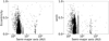 |
Fig. 1 Osculating orbital elements of all objects analyzed in this work with at least one absolute magnitude computed in any filter. |
2 Dataset
We used the data of small bodies extracted from the SDSS, but not the traditional and well-known Moving Objects Catalog (Ivezić et al. 2001; Jurić et al. 2002), which is frozen in its fourth release, with data obtained until March 2007. Instead, we used the re-analysis of the SDSS performed by Sergeyev & Carry (2021), hereafter S21, who released more than one million observations of almost 380 000 small bodies. This multiplied the number of objects with respect to the last release of the Moving Objects Catalog by three.
The S21 catalog includes the point spread function magnitudes in the ugriɀ filter system and their respective uncertainties, σm. We use italics when we discuss magnitudes in the text. S21 also included the heliocentric and topocentric distances of the objects and the phase angle (along with other helpful information). As in Alvarez-Candal et al. (2022a), AC22 hereafter, we did not make any cut in the database other than removing any m with an associated error of σm ≥ 1. We used data of objects with at least three different α and with a minimum span of ∆α ≥ 5.0 deg (i.e., the distance between the maximum and minimum a). Figure 1 shows the distribution in the orbital elements space of all objects with at least one H measured in any filter (see below).
To analyze the data, we built upon the algorithm developed in AC22, with a few modifications intended to improve accuracy, as discussed in the next section.
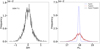 |
Fig. 2 Probability distributions. Left: probability distribution P29030(∆m). Right: example of the final probability distribution. The examples are for asteroid 1034 T-1 or 29030 (MPC designation) with mυ = 17.93 ± 0.06. |
3 Analysis
We used the method described in AC22, updated as described below. The  model (Penttilä et al. 2016) was used as the photometric model because it proved to be better suited to fit the data and because alternative models presented different problems when applied to the S21 dataset. The HG1G2 model (Muinonen et al. 2010) needs a well-sampled phase curve, which is usually not the case of the data analyzed in this work, the Shevchenko model (Belskaya & Shevchenko 2000) needs a good coverage of the phase curve in small phase angles, and the HG model (Bowell et al. 1989) fails to represent the phase curves of high- or low-albedo asteroids. In this case, we did not use the Python adaptation of the
  model provided by the authors, but a code based on the equations presented in Penttilä et al. (2016).
The adopted photometric model describes the phase curves as follows:
![Mathematical equation: $M(\alpha ) = H - 2.5\log \left[ {{G_1}{{\rm{\Phi }}_1}(\alpha ) + {G_2}{{\rm{\Phi }}_2}(\alpha ) + \left( {1 - {G_1} - {G_2}} \right){{\rm{\Phi }}_3}(\alpha )} \right],$](/articles/aa/full_html/2024/05/aa48287-23/aa48287-23-eq4.png) (2)
(2)
where M(α) = m − 5 log (R∆) is the reduced magnitude, H is the absolute magnitude, Φi are known functions of α (see Penttilä et al. 2016 for the tables), and Gi are the phase coefficients that provide the shape of the curve. In the  model, G1 and G2 are parameterized by
  according to
  and
and  . From now on,
  is G for simplicity unless explicitly stated otherwise, and we do not use subindexes to differentiate among filters unless necessary.
Probability distribution function of ∆m. We followed a similar approach as in AC22, with one modification. Alvarez-Candal et al. (2022a) did not include any effect due to the possible rotational phase at which the objects could have been observed; this produced an artifact, a dip, in PA(∆m), as shown in Fig. 2 of AC22. The dip is alleviated when convolving with the errors in the apparent magnitudes, but it still assigned a lower probability than real to the region around ∆m = 0. We changed the code to account for this by multiplying a random sin(ϕ), where ϕ ∊ [0, 2π), simulating an observation at an unknown rotational phase. Equation (2) in AC22 is then rewritten as
 (3)
(3)
where  is the probability denstity function, PDF, of ∆m for object A in 150 bins of width 0.02 mag, meant to cover the whole range of the reported ∆m ∊ [0.0, 3.0] (Warner et al. 2019). The denominator is a normalization factor. With this procedure, we created a PDF of possible values of ∆m that the object could have (see an example in Fig. 2 for asteroid 290301).
The rest of the process was the same as in AC22. We also included the uncertainty in the measurement of m to create the final PDF used to estimate the final range of possible solutions of H in all filters. Therefore, we constructed for each object and measure the distribution, PA(m), as a normal distribution with σ = σm centered at m. The final PDF is the convolution of PA(m) and Eq. (3):
 (4)
(4)
One advantage of including a factor sin (ϕ) in Eq. (3) is that it is not necessary to mirror and rescale PA(m, ∆m), as AC22 needed to do, because now the distribution naturally covers the whole space of possible ∆m.
Computation of the phase curve. As in AC22, we computed H and G for each object and filter using Eq. (2). We generated different solutions of the PCs by randomly extracting 10 000 values from PA(m, ∆m). The method is explained in full in AC22.
The outcome of the processing is the PDF of Hλ and their corresponding Gs if there are at least 100 valid, that is, physically possible solutions. All PDFs are available upon request or in the Open Science Framework (OSF) project folder 43eny2. Table 1 shows a sample of the nominal values of the quantities and their uncertainties. The former is the median of the PDFs, and the uncertainty range indicates the 16th and 84th percentiles. The complete table is available at the CDS.
Sample of the catalog.
4 Results and discussion
Following the above procedure, we computed H in all filters available in the S21 data (see the numbers in Table 2) and also in the HV and HR using 𝑔, r, and i for each α when the magnitudes were available. The data were processed the same way as all the rest using V and R and their corresponding α.
Most objects have fewer than 10 observations, with a median of 4 observations per filter. More than 100 objects have more than 20 observations, and one object was observed 70 times in the g, r, and i filters (Fig. 3, left panel). Most of the objects were observed with αmin < 10 deg with a median span, ∆α, of 8.3 deg (Fig. 3, right panel). The vast majority of objects are main belt asteroids (Fig. 1), but there are objects with a > 100 AU at high eccentricities to fulfill the criteria set above to compute the PC.
The distributions of absolute magnitudes and G are shown in Fig. 4. As was reported in AC22, the Hu distribution peaks at about two magnitudes fainter than in the other filters (compatible with the solar (u − 𝑔) = 1.43). The G distributions all peak at about 0.6 with a full witdh at half maximum, FWHM of about 0.2. There are no apparent changes with wavelength, other than a slight width increase toward bluer wavelengths.
The computed H𝑔 − Hi, H𝑔 − Hr, and Hi − Hɀ are displayed in Fig. 5 in color–color diagrams using density plots to simplify the figures. Overall, the distributions follow the same trend as in previous works (for example Alvarez-Candal et al. 2022a; Colazo et al. 2022; Sergeyev et al. 2023). It is worth mentioning that several objects seem to escape from the usual phase space because they have large uncertainties in their colors (seen as faint clouds in Fig. 5), and care must be taken when using this database.
Number of absolute magnitudes obtained.
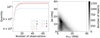 |
Fig. 3 Observational circumstances of the data used in this work. Left panel: cumulative distribution of the number of observations per filter for the objects in this work. Right panel: minimum α vs. span in α covered by the objects in this work. |
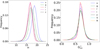 |
Fig. 4 Distributions of computed quantities. Distributions of H (left panel) and G (right panel), u is shown as the blue line, g is shown in green, r is shown in red, i is shown in purple, and ɀ is shown in black. |
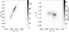 |
Fig. 5 Color–color diagrams in the form of density plots. The left panel shows H𝑔 − Hr vs. H𝑔− Hi, highlighting the linear part of the spectrum, and the right panel shows the H𝑔 − Hi vs. Hi − Hɀ, doing the same for the region that encompasses the 900 nm absorption feature due to silicates. |
4.1 Spectral slope
Alvarez-Candal et al. (2022a) established that the method was reliable, and it provided comparable results with other methods used to compute H (e.g., Oszkiewicz et al. 2011 or Vereš et al. 2015). Therefore, we proceed with the central issue of this article: Phase coloring.
We first computed the spectral slope (slope for short) at different or for all objects with Hu, H𝑔, Hr, and Hi using a simple linear fit to the computed fluxes (see Eq. (5)). Hɀ was excluded from the fit because it falls on the silicate absorption feature in some objects, departing from the linear part of the spectrum.
The fluxes were computed using
![Mathematical equation: ${F_\lambda }(\alpha ) = {10^{ - 0.4\left[ {\left( {\left( {{M_\lambda } - {M_{\rm{r}}}} \right)(\alpha ) - {{\left( {{M_\lambda } - {M_{\rm{r}}}} \right)}_ \odot }} \right]} \right.}}{\rm{,}}$](/articles/aa/full_html/2024/05/aa48287-23/aa48287-23-eq19.png) (5)
(5)
where the solar colors were taken from the SDSS3. In Eq. (5), the object color appears as an explicit function of the phase angle. The color was computed using the nominal values of Hs and Gs, which were fed into Eq. (2). The computation was made in steps of 0.5 deg between or α ∊ [0, 35] deg. Figure 6 shows the results for 42 168 objects. The y-axis shows a normalized spectral slope to facilitate comparison. This slope is computed as
 (6)
(6)
where ∆S = max[S (α) − S 0] − min[S (α) − S 0], and S 0 = S (α = 0 deg). It is immediately clear that there are two types of curves: (i) some slopes decrease with α until a critical value αc, and then revert the behavior (the BR group); (ii) other curves increase the slopes until a critical value, and then start to decrease (the RB group). αc seems to lie between 4.5 and 5 deg in all cases. Behavior BR occurs for 22 858 objects, and behavior RB occurs for 19 310. There are no flat curves. Therefore, an object belongs either to the BR or the RB group. In practice, when the normalization factor in Eq. (6) is removed, some curves will appear flat due to the small amplitude of ∆S. To highlight the maximum change in S (α), we plot a histogram with the distribution of ∆S, as defined above, in Fig. 6 (left). It is clear that most objects do not display a radical change of S(α); the median value is 0.47 × 10⁻⁴ nm-1, which is within the usual uncertainties in the measurements of spectral slopes. Nevertheless, it is important to note that there are almost 300 objects with ∆S > 5 × 10⁻⁴ nm-1, which is well above the typical uncertainties. In any case, we would like to stress that the results displayed in Fig. 6 should be taken as a toy model representation of the results, as the figure does not include the full information in the probability distributions, although it is useful to show different phase-coloring behaviors.
The above results were obtained using the modeled data, which did not account for realistic observations. To add more reality, we conducted a second experiment using the full probability distribution of each absolute magnitude. We extracted 1000 different random values from each H and its corresponding G, and we obtained a distribution of slopes per object and α. In this case, Fig. 6 cannot be reproduced because of the noise in the solutions. Nevertheless, by inspecting some of the resulting curves visually, the behavior is discernible in high-quality data (Fig. 7).
Based on the results shown in Figs. 6 and 7, we decided to separate the sample into two regimes and computed the change in the slope (S′α) with phase angle between 0 and 4.5 deg, and between 5.0 and 35 deg. S′α was computed by a linear fit to S(α) versus α in both cases. The results of both cases were clipped (at 3σ) to remove outliers. The results are shown in Fig. 8. The left panel shows a priori no relation between S′α and S0. The Spearman test shows that there is a weak negative anticorrelation with a rs = −0.01 and a p-value of 0.0026, in a way resembling (though much weaker) the anticorrelation detected for asteroids at small phase angles by Alvarez-Candal et al. (2022b) with a different photometric model. The right panel of the figure shows that above 4.5 deg, the general tendency is for objects to become redder when they are intrinsically redder in opposition.
In the next step, we checked for the coloring behavior in different bins of semimajor axes. The data were split into eight regions: (i) a < 2.05 AU, (ii) 2.05 < a < 2.5 AU, (iii) 2.5 < a < 2.82 AU, (iv) 2.82 < a ≤ 3.3 AU, (v) 3.3 < a ≤ 3.7 AU, (vi) 3.7 < a ≤ 4.5 AU, (vii) 4.5 < a ≤ 5.5 AU, and (viii) a > 5.5 AU. We computed the average S (α) − S 0 value within each region per phase angle bin. The results are shown in Fig. 9. The figure clearly shows that the behavior of the average relative slope is not monotonic with phase angle or in the semimajor axis. Most curves show a reddening of the slopes up to 4.5 deg, and then, the relative slope decreases. The only odd behavior occurs in the semimajor axis occupied by the Jovian Trojans, 4.4–5.5 AU, where there is bluing and then reddening of the relative slopes. We checked that the distribution of α is similar in all semimajor axis bins to avoid introducing undesired biases.
The uncertainties of the quantities were not considered to avoid blurring the results too much. We note, however, that the uncertainties were computed for the realistic slope as the standard deviation of the distributions and are available in the OSF folder.
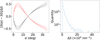 |
Fig. 6 Two behaviors of the spectral slope. Left: change in the spectral slope relative to the slope at α = 0 deg and normalized to its maximum amplitude to increase contrast. The continuous line shows the average value of all objects with that behavior, and the dashed lines indicate the maximum and minimum values per α bin. Right: distribution of ∆S. |
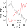 |
Fig. 7 Change in the spectral slope relative to the slope at α = 0 deg and normalized to its maximum amplitude to increase contrast using the full P(Hλ). With the continuous red line, we show the curve for 29030, whose colors might mean that it is an S-complex asteroid, see below, and with the dot-dashed black line, we show the curve for 37478, a possible C-complex asteroid according to its colors. |
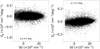 |
Fig. 8 Change in the spectral slope (S′α) with respect to the spectral slope at opposition, 50. Left: S′α computed for α ≤ 4.5 deg. Right: S′α computed for α > 4.5 deg. |
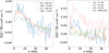 |
Fig. 9 Average relative spectral slope in bins of semimajor axis. The results for each bin are marked within the figures. |
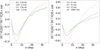 |
Fig. 10 Average relative Hi − Hɀ in bins of semimajor axis. The results for each bin are marked within the figures. |
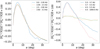 |
Fig. 11 Average relative H𝑔 − Hi in bins of semimajor axis. The results for each bin are marked within the figures. |
4.2 Colors and phase angle
Not only the evolution of the slope with α is interesting. We also studied the change in the colors with the phase angle. Following a similar procedure as above to compute the more realistic slopes, we used the average relative color in the same semimajor axis bins as above and show the results for the Hi − Hɀ in Fig. 10 and for H𝑔 − Hi in Fig. 11 The behavior of Hi − Hɀ indicates that the color decreases until about 5 deg in all semimajor axis bins on average, and it increases and becomes redder with increasing α. Objects of all taxa were included in the averaging.
On the other hand, H𝑔 − Hi seems to follow the curves of the average relative slope (Fig. 9), which is natural because this region is less affected by the 900 nm absorption band. Overall, the color seems to increase until the critical angle, and then the color starts to decrease after αc. The same trends are seen in all semimajor axis bins, while the Hilda and Trojan regions have less dramatic changes.
As mentioned, the uncertainties of the quantities were not included to avoid blurring the results. Nevertheless, the uncertainties were computed as the interval between the 16th and the 84th percentile of the convolution of the PDFs of the colors, as explained in Sect. 3.2 of Alvarez-Candal et al. (2022b). These uncertainties are available in the OSF folder.
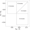 |
Fig. 12 Schematic view of the boxes considered for each taxon. |
Relative change in the taxa.
4.3 Impact on the taxonomy classes
The previous sections established that spectral slopes and colors change with the phase angle. The next step is to verify whether these changes are sufficient to change the taxon of an object. To do this, a simple experiment was performed using the four taxa defined by Colazo et al. (2022), that is, the C, X, S, and V complexes. We crudely separated the H𝑔 − Hi versus Hi − Hɀ into the four regions that are covered by each taxon (Fig. 12 provides a schematic view). The C-complex is located in H𝑔 − Hi ∊ (0.47, 0.727) ∧ Hi − Hɀ ∊ (−0.128, 0.25), the X-complex is located in H𝑔 − Hi ∊ (0.727, 1.05) ∧ Hi − Hɀ ∊ (1.129[H𝑔 − Hi] − 0.926, 0.25), and the S-complex is located in in H𝑔 − Hi ∊ (0.727, 1.05) Λ Hi − Hɀ ∊ (−0.128, 1.129[H𝑔 − Hi] − 0.926). Finally, the V-complex is located in H𝑔 − Hi ∊ (0.727, 1.05) Λ Hi − Hɀ ∊ (−0.478, −0.128).
We computed the number of objects in each box at α = 0 deg, N0, the number Nc at αc, and the number of objects, Nm, at the maximum phase angle (αmax). According to Figs. 10 and 11, the maximum differences in color should occur between αc and αmax. The results are shown in Table 3, where the differences are expressed per mille.
As expected, the largest changes occur between Nc and Nm. Curiously, the V-complex alone loses objects from opposition to αc to increment their numbers from αc to αmax. In any case, this is a rough estimate that provides minimum numbers because the space covered by each box is larger than the actual taxon should occupy, and we did not follow any particular object either, but just counted the number of objects at each step. It is therefore likely that between steps, more objects moved in or out of each region (see also Appendix A).
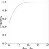 |
Fig. 13 Cumulative distribution of αmin − αw (see text for a description of both angles). |
4.4 Use of weighted averages
Weighted arithmetic averages are commonly used to compute colors (and other quantities) of Solar System objects (for example Hainaut et al. 2012; Sergeyev et al. 2023). The idea behind this approach is to prioritize data with high precision, the usual weight being the inverse of the uncertainty (or square uncertainty). This approach is valid if, and only if, all data are compatible. In this case, we mean by compatible that all measurements were taken at the same phase angle, distances to the Sun and Earth, and rotational phase. Otherwise, some systematic may be introduced because the objects tend to become brighter closer to the opposition, which presumably increases the precision of the measurements.
We examined the data for S21 and used the same criteria as mentioned above to select the data, but in this case, computing the weighted average in u − 𝑔, 𝑔 − r, r − i, and i − ɀ and then comparing these averaged value with the individual colors at each value of α and saved the phase angle (called αw) where they were closer. Then, we compared the value of αw with the minimum phase angle for each object. The results displayed in Fig. 13 correspond to the 𝑔 − r color measurements and are similar in the other colors. In the figure, it is clear that using a weighting scheme biases the colors toward low-phase angles (i.e., closer to opposition): 50% of the average colors coincide with the minimum α in the phase curve within 1 deg, while three-quarters of the sample are within 5 deg of the minimum phase angle. Therefore, we recommend care when using averaged values because these values are biased so that low-phase angle measurements carry more weight. To further complicate the interpretation of results obtained with average colors, Alvarez-Candal et al. (2022a) showed that the average colors and the colors at opposition (i.e., the difference of the absolute magnitudes that we call absolute colors) can have significant differences and that there is no one-to-one correspondence between them.
5 Conclusions
The terminology phase reddening has been used for a while to describe an observational effect: Objects observed at higher phase angles tended to have redder colors (or steeper spectral slopes Luu & Jewitt 1990, for instance). Nevertheless, this was usually seen in a relatively low number of objects because traditional observation programs were not efficient in scheduling repeated observations of the same object in different phase angles. For example, Nathues (2010) reported from a sample of over 90 Eunomia objects that only six objects had two or more observations, including one with a clear bluing: (5785) Fulton.
The results we showed in this paper point to different behaviors in different phase-angle regimes: In terms of spectral slope, there seems to be a slight anticorrelation between S′α computed for α ≤ 4.5 deg and S 0, suggesting that intrinsically redder objects tend to become slightly bluer with increasing phase angle, while the opposite is seen for intrinsically bluer objects (see Fig. 8). These results are strikingly similar to the results of Ayala-Loera et al. (2018) for TNOs and Alvarez-Candal et al. (2022b) for asteroids. On the other hand, S′α for α > 5 deg shows that intrinsically redder objects tend to become redder on average, which is in line with the traditional view of phase coloring.
There also seem to be two behaviors in terms of spectral slopes with respect to α (Figs. 6, 7, and 9): The objects tend to have one behavior in the range [0, 4.5] deg and the opposite behavior in the range [4.5, 35] deg. There seems to be a slight predominance of objects that increase the spectral slope and then become bluer, the RB group. This behavior occurs in almost all semimajor axis bins, but the effect is within the error bars in typical spectral slope measurements (the unit [104 nm-1] is equivalent to [% (1000 Å)-1]). We also cross-matched the data with the taxa determined by Colazo et al. (2022) to determine whether the two behaviors might be related to the surface composition, but we found no evidence of this. In Appendix B we distinguish the behavior of the RB and BR groups to analyze their different demeanor.
Color-wise, there are similar behaviors: they first go in one direction to then suddenly change to the opposite. The H𝑔 − Hi correlates with the slope, which is expected because the i filter falls in a region that is relatively unaffected by absorption features. We find the behavior of the Hi − Hɀ more interesting because it targets the absorption band at 900 nm due to silicates. In this case, the color becomes bluer for α ∊ [0, 4.5] deg, while the average color increases for α > 4.5 deg. This means that the band becomes deeper or shallower in objects with an absorption feature just by phase coloring. When the results for both colors, H𝑔 − Hi and Hi − Hɀ, are joined, there seem to be objects that become more concave for low-α and less concave for a higher phase angle. Once again, we stress the orders of magnitude of the effect, which is about one-hundredth of a magnitude at most.
One interesting point to consider is that αc coincides roughly with the onset of the nonlinear part of the PC, where the opposition effect (OE) lies. The OE occurs due to a combination of shadow-hiding (Hapke 1963) and coherent back-scattering (Muinonen 1989) and produces a net increase in the brightness of the object when observed close to opposition (α ≈ 0 deg). The effect starts to appear below 5–6 deg (Belskaya & Shevchenko 2000), but it can start as close to the opposition as below 1 deg (for example, in trans-Neptunian objects, see, Verbiscer et al. 2022). The apparent coincidence is very suggestive, and it deserves further analysis beyond the scope of this work. Perhaps the physical explanation for the phenomena described in this work lie here: which scattering mechanism dominates, and how it behaves with the wavelength. Unfortunately, we cannot yet provide a satisfactory answer.
The effects we report in this paper are unlikely to change how we see the taxa distribution of small bodies in the Solar System (for example Mothé-Diniz et al. 2003; DeMeo & Carry 2013; Marsset et al. 2022; Sergeyev et al. 2023), at least not for the core of the groups, but it does add noise to the frontiers between taxa where some objects do change taxa. The numbers are small to begin with, in the range of a few dozen per thousand. Nevertheless, with the arrival of massive multiwavelength photometric surveys, this may change because the precision in the measurements may reach the level of the measurements shown in this work or be close to this level. On the other hand, with the large numbers, we can now statistically study the phase-related behavior of many objects, which enables an analysis that was impossible before.
Acknowledgements
I am grateful to an anonymous reviewer who provided useful comments that helped improve this draft. A.A.C. acknowledges financial support from the Severo Ochoa grant CEX2021-001131-S funded by MCIN/AEI/10.13039/501100011033. Funding for the creation and distribution of the SDSS Archive has been provided by the Alfred P. Sloan Foundation, the Participating Institutions, the National Aeronautics and Space Administration, the National Science Foundation, the U.S. Department of Energy, the Japanese Monbukagakusho, and the Max Planck Society. The SDSS Web site is http://www.sdss.org/. The SDSS is managed by the Astrophysical Research Consortium (ARC) for the Participating Institutions. The Participating Institutions are The University of Chicago, Fermilab, the Institute for Advanced Study, the Japan Participation Group, The Johns Hopkins University, the Korean Scientist Group, Los Alamos National Laboratory, the Max-Planck-Institute for Astronomy (MPIA), the Max-Planck-Institute for Astrophysics (MPA), New Mexico State University, University of Pittsburgh, University of Portsmouth, Princeton University, the United States Naval Observatory, and the University of Washington. I am grateful to the anonymous reviewer of AC22 who inspired the modification of the algorithm shown in Sect. 3. This work used https://www.python.org/,https://numpy.org (Harris et al. 2020), https://www.scipy.org/,andMatplotlib (Hunter 2007). All figures in this work can be reproduced using the following Colab Notebook https://colab.research.google.com/drive/1-UhSr44YuOAgwMfr-YoWsGztx-QYqgxX?usp=sharing.
Appendix A Evolution of taxa with α
The change in spectral slope and colors, as seen in Sects. 4.1 and 4.2, predicts that objects may change their taxon due to changes in α. In Sect. 4.3 we made a crude estimate of the fractional changes in four defined boxes, representing the four major complexes C, X, S, and V. As mentioned, there was no attempt to track the behavior of particular objects, however. In Figs. A.1 to A.4, we explicitly show how objects that initially are in one of the boxes evolve with changing α: from opposition to αc, and from αc to αmax = 35 deg.
It is clear that most changes in taxonomic assignment occur in the limiting regions between boxes and that some objects may change significantly, although the bulge of the population stays within the borders. In the figures, any object leaving the regions limited by the boxes is labeled as unclassified.
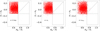 |
Fig. A.1 Evolution of asteroids within the C-complex at α = 0 deg with changing phase angle. Left: Initial conditions. Middle: α = αc. Right: α = αmax. |
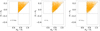 |
Fig. A.2 Evolution of asteroids within the X-complex at α = 0 deg with changing phase angle. Left: Initial conditions. Middle: α = αc. Right: α = αmax. |
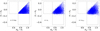 |
Fig. A.3 Evolution of asteroids within the S-complex at α = 0 deg with changing phase angle. Left: Initial conditions. Middle: α = αc. Right: α = αmax. |
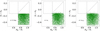 |
Fig. A.4 Evolution of asteroids within the V-complex at α = 0 deg with changing phase angle. Left: Initial conditions. Middle: α = αc. Right: |
Appendix B The two behaviors
In Sect. 4.1 we detected that the slopes of the asteroids follow two different behaviors (in two different regimes): the BR group first becomes bluer until αc, to become redder for larger α. In contrast, the opposite holds for the RB group. In this appendix, we explore how the two groups behave in the different plots shown in the main text, namely Figs. 8 to 11.
We first analyze the behavior of the change in S′α with respect to S 0. In this case, we separated the objects into blue and red dots according to whether their behavior was to become blue or red, according to Fig. 6. In this case, we used as in Fig. 8 the total probability distributions of Hs and Gs to better understand the impact of the observational results. For both groups, the behavior is the same at α > αc: Intrinsically redder objects tend to increase their slope faster than intrinsically bluer objects. In both cases, the Spearman rank order test predicts correlated quantities with p-values virtually equal to zero. On the other hand, the slopes below the critical angle tend to increase with S 0 for the BR group, while they seem to decrease slightly for the RB group. In both cases, the Spearman index rS < |0.1|.
The following figure (Fig. B.2 is analogous to Fig. 9) shows the average slope changes in different bins of the semimajor axis (as discussed in the text). In this case, and as expected, we detect both behaviors when the BR and RB groups were separated. However, the scales of the average changes are more significant than when all objects are considered together. This suggests that the effect tends to cancel out when all objects are included, with a slight dominance of the RB group.
The colors Hi − Hz and Hg − Hi show that the latter correlates with the spectral slopes, as expected (Fig. B.3). Perhaps the most exciting difference comes from the former color, which changes its overall behavior according to whether the objects are from the RB or the BR groups. The BR objects first increase in color and then decrease in it, while the opposite is seen for the RB group (Fig. B.4); in a way, the color is anticorrelated with the change in slope or Hg− Hi.
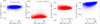 |
Fig. B.1 S′(α) vs. 50. Left panels: BR group. Right panels: RB group. |
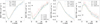 |
Fig. B.2 Average slope for different semimajor axis bins. Left panels: BR group. Right panels: RB group. |
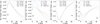 |
Fig. B.3 Average Hi − Hz vs. α. Left panels: BR group. Right panels: RB group. |
 |
Fig. B.4 Average Hg − Hi vs. α. Left panels: BR group. Right panels: RB group. |
The results shown for the colors indicate that for the BR objects, the photo-spectra first become flatter and perhaps slightly convex on average, to then become slightly concave. The RB group goes in the other direction, however.
References
- Alvarez-Candal, A., Benavidez, P. G., Campo Bagatin, A., & Santana-Ros, T. 2022a, A&A, 657, A80 [NASA ADS] [CrossRef] [EDP Sciences] [Google Scholar]
- Alvarez-Candal, A., Jimenez Corral, S., & Colazo, M. 2022b, A&A, 667, A81 [NASA ADS] [CrossRef] [EDP Sciences] [Google Scholar]
- Ayala-Loera, C., Alvarez-Candal, A., Ortiz, J. L., et al. 2018, MNRAS, 481, 1848 [NASA ADS] [CrossRef] [Google Scholar]
- Belskaya, I. N., & Shevchenko, V. G. 2000, Icarus, 147, 94 [NASA ADS] [CrossRef] [Google Scholar]
- Bowell, E., & Lumme, K. 1979, Colorimetry and Magnitudes of Asteroids., eds. T. Gehrels, & M. S. Matthews, 132 [Google Scholar]
- Bowell, E., Hapke, B., Domingue, D., et al. 1989, in Asteroids II, eds. R. P. Binzel, T. Gehrels, & M. S. Matthews, 524 [Google Scholar]
- Carry, B. 2018, A&A, 609, A113 [NASA ADS] [CrossRef] [EDP Sciences] [Google Scholar]
- Colazo, M., Duffard, R., & Weidmann, W. 2021, MNRAS, 504, 761 [NASA ADS] [CrossRef] [Google Scholar]
- Colazo, M., Alvarez-Candal, A., & Duffard, R. 2022, A&A, 666, A77 [NASA ADS] [CrossRef] [EDP Sciences] [Google Scholar]
- DeMeo, F. E., & Carry, B. 2013, Icarus, 226, 723 [NASA ADS] [CrossRef] [Google Scholar]
- Fukugita, M., Ichikawa, T., Gunn, J. E., et al. 1996, AJ, 111, 1748 [Google Scholar]
- Grynko, Y., & Shkuratov, Y. G. 2008, Light Scattering from Particulate Surfaces in Geometrical Optics Approximation, ed. A. A. Kokhanovsky (Berlin, Heidelberg: Springer Berlin Heidelberg), 329 [Google Scholar]
- Hainaut, O. R., Boehnhardt, H., & Protopapa, S. 2012, A&A, 546, A115 [NASA ADS] [CrossRef] [EDP Sciences] [Google Scholar]
- Hapke, B. W. 1963, J. Geophys. Res., 68, 4571 [NASA ADS] [CrossRef] [Google Scholar]
- Harris, C. R., Millman, K. J., van der Walt, S. J., et al. 2020, Nature, 585, 357 [NASA ADS] [CrossRef] [Google Scholar]
- Hunter, J. D. 2007, Comput. Sci. Eng., 9, 90 [NASA ADS] [CrossRef] [Google Scholar]
- Ivezić, Ž., Tabachnik, S., Rafikov, R., et al. 2001, AJ, 122, 2749 [Google Scholar]
- Ivezić, Ž., Kahn, S. M., Tyson, J. A., et al. 2019, ApJ, 873, 111 [Google Scholar]
- Jones, R. L., Chesley, S. R., Connolly, A. J., et al. 2009, Earth Moon Planets, 105, 101 [NASA ADS] [CrossRef] [Google Scholar]
- Jurić, M., Ivezic, Ž., Lupton, R. H., et al. 2002, AJ, 124, 1776 [CrossRef] [Google Scholar]
- Luu, J. X., & Jewitt, D. C. 1990, AJ, 99, 1985 [NASA ADS] [CrossRef] [Google Scholar]
- Mahlke, M., Carry, B., & Denneau, L. 2021, Icarus, 354, 114094 [Google Scholar]
- Marsset, M., DeMeo, F. E., Burt, B., et al. 2022, AJ, 163, 165 [NASA ADS] [CrossRef] [Google Scholar]
- Millis, R., Bowell, E., & Thompson, D. 1976, Icarus, 28, 53 [NASA ADS] [CrossRef] [Google Scholar]
- Mothé-Diniz, T., Carvano, J. M. á., & Lazzaro, D. 2003, Icarus, 162, 10 [CrossRef] [Google Scholar]
- Muinonen, K. 1989, Appl. Opt., 28, 3044 [NASA ADS] [CrossRef] [Google Scholar]
- Muinonen, K., Belskaya, I. N., Cellino, A., et al. 2010, Icarus, 209, 542 [Google Scholar]
- Nathues, A. 2010, Icarus, 208, 252 [NASA ADS] [CrossRef] [Google Scholar]
- Nelson, R. M., Hapke, B. W., Smythe, W. D., & Horn, L. J. 1998, Icarus, 131, 223 [NASA ADS] [CrossRef] [Google Scholar]
- Oszkiewicz, D., Muinonen, K., Bowell, E., et al. 2011, JQSRT, 112, 1919 [NASA ADS] [CrossRef] [Google Scholar]
- Penttilä, A., Shevchenko, V. G., Wilkman, O., & Muinonen, K. 2016, Planet. Space Sci., 123, 117 [Google Scholar]
- Popescu, M., Licandro, J., Morate, D., et al. 2016, A&A, 591, A115 [NASA ADS] [CrossRef] [EDP Sciences] [Google Scholar]
- Sanchez, J. A., Reddy, V., Nathues, A., et al. 2012, Icarus, 220, 36 [CrossRef] [Google Scholar]
- Sergeyev, A. V., & Carry, B. 2021, A&A, 652, A59 [NASA ADS] [CrossRef] [EDP Sciences] [Google Scholar]
- Sergeyev, A. V., Carry, B., Marsset, M., et al. 2023, A&A, 679, A148 [NASA ADS] [CrossRef] [EDP Sciences] [Google Scholar]
- Shkuratov, Y., Ovcharenko, A., Zubko, E., et al. 2002, Icarus, 159, 396 [CrossRef] [Google Scholar]
- Taylor, R. C., Gehrels, T., & Silvester, A. B. 1971, AJ, 76, 141 [Google Scholar]
- Verbiscer, A. J., Helfenstein, P., Porter, S. B., et al. 2022, Planet. Sci. J., 3, 95 [NASA ADS] [CrossRef] [Google Scholar]
- Vereš, P., Jedicke, R., Fitzsimmons, A., et al. 2015, Icarus, 261, 34 [CrossRef] [Google Scholar]
- Warner, B., Pravec, P., & Harris, A. P. 2019, Asteroid Lightcurve Data Base (LCDB) V3.0 urn:nasa:pds:ast-lightcurve-database::3.0, NASA Planetary Data System, Available at https://sbn.psi.edu/pds/resource/lc.html [Google Scholar]
- Wolf, C., Onken, C. A., Luvaul, L. C., et al. 2018, PASA, 35, e010 [Google Scholar]
- York, D. G., Adelman, J., Anderson, John E., J., et al. 2000, AJ, 120, 1579 [NASA ADS] [CrossRef] [Google Scholar]
The asteroid 29030, or 1034 T-1, is used as an example because it was already used in AC22 and Alvarez-Candal et al. (2022b).
All Tables
All Figures
|
Fig. 1 Osculating orbital elements of all objects analyzed in this work with at least one absolute magnitude computed in any filter. |
| In the text | |
|
Fig. 2 Probability distributions. Left: probability distribution P29030(∆m). Right: example of the final probability distribution. The examples are for asteroid 1034 T-1 or 29030 (MPC designation) with mυ = 17.93 ± 0.06. |
| In the text | |
|
Fig. 3 Observational circumstances of the data used in this work. Left panel: cumulative distribution of the number of observations per filter for the objects in this work. Right panel: minimum α vs. span in α covered by the objects in this work. |
| In the text | |
|
Fig. 4 Distributions of computed quantities. Distributions of H (left panel) and G (right panel), u is shown as the blue line, g is shown in green, r is shown in red, i is shown in purple, and ɀ is shown in black. |
| In the text | |
|
Fig. 5 Color–color diagrams in the form of density plots. The left panel shows H𝑔 − Hr vs. H𝑔− Hi, highlighting the linear part of the spectrum, and the right panel shows the H𝑔 − Hi vs. Hi − Hɀ, doing the same for the region that encompasses the 900 nm absorption feature due to silicates. |
| In the text | |
|
Fig. 6 Two behaviors of the spectral slope. Left: change in the spectral slope relative to the slope at α = 0 deg and normalized to its maximum amplitude to increase contrast. The continuous line shows the average value of all objects with that behavior, and the dashed lines indicate the maximum and minimum values per α bin. Right: distribution of ∆S. |
| In the text | |
|
Fig. 7 Change in the spectral slope relative to the slope at α = 0 deg and normalized to its maximum amplitude to increase contrast using the full P(Hλ). With the continuous red line, we show the curve for 29030, whose colors might mean that it is an S-complex asteroid, see below, and with the dot-dashed black line, we show the curve for 37478, a possible C-complex asteroid according to its colors. |
| In the text | |
|
Fig. 8 Change in the spectral slope (S′α) with respect to the spectral slope at opposition, 50. Left: S′α computed for α ≤ 4.5 deg. Right: S′α computed for α > 4.5 deg. |
| In the text | |
|
Fig. 9 Average relative spectral slope in bins of semimajor axis. The results for each bin are marked within the figures. |
| In the text | |
|
Fig. 10 Average relative Hi − Hɀ in bins of semimajor axis. The results for each bin are marked within the figures. |
| In the text | |
|
Fig. 11 Average relative H𝑔 − Hi in bins of semimajor axis. The results for each bin are marked within the figures. |
| In the text | |
|
Fig. 12 Schematic view of the boxes considered for each taxon. |
| In the text | |
|
Fig. 13 Cumulative distribution of αmin − αw (see text for a description of both angles). |
| In the text | |
|
Fig. A.1 Evolution of asteroids within the C-complex at α = 0 deg with changing phase angle. Left: Initial conditions. Middle: α = αc. Right: α = αmax. |
| In the text | |
|
Fig. A.2 Evolution of asteroids within the X-complex at α = 0 deg with changing phase angle. Left: Initial conditions. Middle: α = αc. Right: α = αmax. |
| In the text | |
|
Fig. A.3 Evolution of asteroids within the S-complex at α = 0 deg with changing phase angle. Left: Initial conditions. Middle: α = αc. Right: α = αmax. |
| In the text | |
|
Fig. A.4 Evolution of asteroids within the V-complex at α = 0 deg with changing phase angle. Left: Initial conditions. Middle: α = αc. Right: |
| In the text | |
|
Fig. B.1 S′(α) vs. 50. Left panels: BR group. Right panels: RB group. |
| In the text | |
|
Fig. B.2 Average slope for different semimajor axis bins. Left panels: BR group. Right panels: RB group. |
| In the text | |
|
Fig. B.3 Average Hi − Hz vs. α. Left panels: BR group. Right panels: RB group. |
| In the text | |
|
Fig. B.4 Average Hg − Hi vs. α. Left panels: BR group. Right panels: RB group. |
| In the text | |
Current usage metrics show cumulative count of Article Views (full-text article views including HTML views, PDF and ePub downloads, according to the available data) and Abstracts Views on Vision4Press platform.
Data correspond to usage on the plateform after 2015. The current usage metrics is available 48-96 hours after online publication and is updated daily on week days.
Initial download of the metrics may take a while.