© The Authors 2024

1. Introduction

Up to this point, terrestrial gravitational wave (GW) observatories have detected only binary mergers of stellar compact objects (Abbott et al. 2019, 2021; LIGO Scientific Collaboration et al. 2023). The signal from these sources remains discrete, in the sense that it does not overlap with the signal from another source when detected. This is expected to change in the future (Maggiore et al. 2020; Amaro-Seoane et al. 2017), when GW observatories are expected to receive signals from multiple sources simultaneously. A more extreme case of such overlap is seen when the sources are so numerous that one cannot be discerned from another, creating a stochastic GW background (SGWB).

There are several types of SGWBs depending on their sources (Boileau et al. 2021; Martinovic et al. 2021; Agazie et al. 2023; Afzal et al. 2023; Antoniadis et al. 2024); they can be split into two categories: cosmological sources and astrophysical sources. The latter category contains mainly different types of compact binary coalescences, but also hyperbolic encounters of compact objects. Contrary to the compact binary coalescences for which the signal can last for many cycles, in the case of hyperbolic encounters the signal can be viewed rather as a transient (Morrás et al. 2022). The peak of this transient GW signal lies near the pericenter of the respective hyperbolic trajectory (De Vittori et al. 2012), which should correspond to short bursts of GWs. The exact waveform of these bursts (Cho et al. 2018; Vines et al. 2019; Jakobsen et al. 2021; Saketh et al. 2022; Chowdhuri et al. 2023) is not relevant for the study of an SGWB, because we are interested in the accumulative effect of many events.

It is often argued that bound compact clusters, such as globular clusters (GCs), can be one of the possible dominant channels for hyperbolic encounters in the Universe (Dymnikova et al. 1982; Kocsis et al. 2006). Therefore, encounters in GCs are expected to provide an adequate number of events for an SGWB (Mukherjee et al. 2021). This rate depends on the number of black holes (BHs) in a cluster and on the number of clusters in a galaxy. Therefore, from an astrophysical point of view, detecting a SGWB or failing to do so would put constraints on the numbers mentioned above.

Our work continues the investigation done by Mukherjee et al. (2021), in which an estimate of the detectable event rates was provided. In particular, we investigate BH hyperbolic encounters where eccentricities tend to be almost parabolic; that is, the eccentricity is very close to one. We obtain different energy density profiles of the SGWB generated by these encounters while varying the parameters of the system, such as the masses of the BHs and the virial velocity in the cluster. The comparison of these profiles with the respective sensitivity curves of GW observatories allows us to infer some preferable scenarios for detection.

The remainder of the article is organized as follows: in Sect. 2 we describe how we modeled the orbital dynamics of the hyperbolic encounters and the respective GW radiation. In Sect. 3 we show how we computed the dimensionless GW energy density spectrum for the hyperbolic encounters. In Sect. 4 we present our results and in Sect. 5 we conclude with a discussion of our main findings.

2. Analytical calculations

2.1. Orbital parameters

In this section, we briefly review the orbital parameters for hyperbolic encounters limited within a radius of a cluster, as given by Mukherjee et al. (2021). This motion is planar and each orbit is determined by its initial conditions: the initial distance r_i between the bodies, the initial angle θ_i between r_i and the initial velocity of the secondary v_i, and the masses of the objects m₁ and m₂ (for an illustration see Fig. 1). As mentioned above, the initial radius is chosen to be less than the cluster radius, that is r_i ≤ R_c, where R_c is the radius of a cluster; v_i is estimated from virial theorem; and θ_i is considered to have an arbitrary value within its physical range¹.

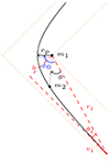Fig. 1. Hyperbolic trajectory of a secondary compact object of mass m2 in the gravitational field of a BH of mass m1. The secondary object is initially located at a distance ri from the primary; the initial angle between the line connecting the bodies and the initial velocity vi is θi. The motion of the secondary can be parametrized by the radial distance r(ϕ) as a function of the azimuthal angle ϕ, where ϕ lies between ri and r(ϕ). The rp is the periapsis, which is the minimum distance between the bodies, and ϕ0 is the periapsis angle, which is the angle between r(ϕ) and rp. As shown here, we define the impact parameter b as the vertical distance between the primary BH and the initial velocity of the secondary; that is, b = ri sin θi.

As the objects are far from each other, we use the Keplerian potential energy. The Hamiltonian for this system is

$$\begin{array}{c}\hfill H=E=\frac{1}{2}(p_r^2+\frac{L^2}{r^2})-\frac{\mathit{GM}}{r},\end{array}$$(1)

where E, p_r, and L are the total energy, the radial momentum, and the total angular momentum per unit of reduced mass μ, while M = m₁ + m₂ is the total mass and 1/μ = 1/m₁ + 1/m₂ is the reduced mass of the system. Moreover, from Fig. 1 the total angular momentum per μ can be written as L = r_iv_i sin θ_i. Solving Hamiltonian (1) allows us to find that

$$\begin{array}{c}\hfill r(\varphi )=\frac{p}{1+ecos(\varphi -{\varphi }_0)},\end{array}$$(2)

where ϕ is the angle between r_i and r(ϕ) and p, e, and ϕ₀ are given by

$$\begin{array}{c}\hfill p=\frac{b^2}{a},e^2=1+\frac{b^2}{a^2}\alpha ,tan{\varphi }_0=-\frac{b}{a}\beta ,\end{array}$$(3)

with

$$\begin{array}{cc}\hfill a& =GM/v_i^2,b=L/v_i,\hfill \\ \hfill \alpha & =1-2a/r_i,\beta =cos{\theta }_i{(1-b^2/(a{r}_i))}^{-1}.\hfill \end{array}$$(4)

See Mukherjee et al. (2021) for a detailed derivation of these quantities².

2.2. Energy radiation in the time domain

As we are dealing with an SGWB, to calculate the gravitation radiation reaction from the hyperbolic encounters, it is reasonable to assume that an estimation of the leading terms of this reaction is sufficient (Roskill et al. 2023). Therefore, we use the quadrupole formula (see, e.g., Maggiore 2007) should be sufficient for the scope of the present work. The quadrupole moment tensor is given by

$$\begin{array}{c}\hfill Q_{\mathit{ij}}=\mu (3x_i{x}_j-\mid r{\mid }^2{\delta }_{\mathit{ij}}),\end{array}$$

where the nonzero components of this system are

$$\begin{array}{cc}\hfill Q_{11}& =\mu r^2(3{cos}^2\varphi -1),\hfill \end{array}$$(5)

$$\begin{array}{cc}\hfill Q_{22}& =\mu r^2(3{sin}^2\varphi -1),\hfill \end{array}$$(6)

$$\begin{array}{cc}\hfill Q_{12}& =Q_{21}=3\mu r^{2}cos\varphi sin\varphi ,\hfill \end{array}$$(7)

$$\begin{array}{cc}\hfill Q_{33}& =-\mu r^2.\hfill \end{array}$$(8)

Then, the power emitted through GW is determined from

$$\begin{array}{cc}\hfill P=& \frac{\mathrm{d}E}{\mathrm{d}t}=-\frac{G}{45c^5}({\stackrel{⃛}{Q}}_{\mathit{ij}}{\stackrel{⃛}{Q}}^{\mathit{ij}})=-\frac{4L^{6}G}{15p^8{\mu }^4{c}^5}{[1+ecos(\varphi -{\varphi }_0)]}^4\hfill \\ \hfill & \{1+13e^2+48ecos(\varphi -{\varphi }_0)+11e^{2}cos(2\varphi -2{\varphi }_0)\}.\hfill \end{array}$$(9)

By substituting the relations (4), we arrive at

$$\begin{array}{c}\hfill P(t)=\frac{\mathrm{d}E}{\mathrm{d}t}=-\frac{32G}{45c^5}\frac{{\mu }^2{\alpha }^4{v}_i^6}{b^2}f(\varphi ,e),\end{array}$$(10)

with

$$\begin{array}{cc}\hfill f(\varphi ,e)& =\frac{3{(1+ecos(\varphi -{\varphi }_0))}^4}{8{(e^2-1)}^4}\{24+13e^2\hfill \\ \hfill & +48ecos(\varphi -{\varphi }_0)+11e^{2}cos2(\varphi -{\varphi }_0)\}.\hfill \end{array}$$(11)

The above expression exactly matches the existing literature, except for α, which arises from the different definitions of a and b (see Appendix A; García-Bellido & Nesseris 2018).

We note that the relation between ϕ and t can be derived from $L=r^2\dot{\varphi }$. To get an explicit relation, one can rewrite this in the form

$$\begin{array}{c}\hfill Lt=p^2{\int }_{\varphi 0}^{\varphi }\frac{\mathrm{d}\varphi }{{[1+ecos(\varphi -{\varphi }_0)]}^2},\end{array}$$(12)

and consequently, we get

$$\begin{array}{cc}\hfill \mathit{Lt}& =-p^2[\frac{2}{{(e^2-1)}^{3/2}}{tanh}^{-1}(\sqrt{\frac{e-1}{e+1}}tan(\frac{\varphi -{\varphi }_0}{2}))]\hfill \\ \hfill +& \frac{p^{2}esin(\varphi -{\varphi }_0)}{(e^2-1)(1+ecos(\varphi -{\varphi }_0))}.\hfill \end{array}$$(13)

2.3. Energy radiation in the frequency domain

To compute the frequency spectrum of the radiated power ΔE, we employ the Fourier transformation (FT) of the energy emission in the time domain; that is,

$$\begin{array}{c}\hfill \mathrm{\Delta }E={\int }_{-\infty }^{+\infty }P(t)\mathrm{d}t=\frac{1}{\pi }{\int }_0^{+\infty }P(\omega )\mathrm{d}\omega ,\end{array}$$(14)

where P(ω) is the power radiation in the frequency domain given by

$$\begin{array}{c}\hfill P(\omega )=\frac{G}{45c^5}\sum _{i,j}\widehat{\stackrel{⃛}{Q_{\mathit{ij}}}}{\widehat{\stackrel{⃛}{Q_{\mathit{ij}}}}}^{\ast },\end{array}$$(15)

and the over-hat represents the FT defined as

$$\begin{array}{c}\hfill \widehat{f(\omega )}={\int }_{-\infty }^{+\infty }f(t){\mathit{e}}^{-i\omega t}\mathrm{d}t.\end{array}$$(16)

Additionally, Eq. (16) implies $\widehat{\dot{f}}=i\omega \widehat{f}$, and consequently $\widehat{\stackrel{⃛}{f}}=-i{\omega }^3\widehat{f}$. For simplicity, we use this relation for Eq. (15) and write it in terms of Q_ij as follows:

$$\begin{array}{c}\hfill P(\omega )=\frac{G{\omega }^6}{45c^5}\widehat{Q_{\mathit{ij}}}{\widehat{Q_{\mathit{ij}}}}^{\ast }.\end{array}$$(17)

The radial trajectory given in Eq. (2) is a function of ϕ and the dependence of ϕ in terms of t is given by Eq. (13). However, this parameterization is not suitable if the FT is going to be applied. Therefore, we reparameterize the hyperbolic trajectory in terms of the eccentric anomalyξ as follows:

$$\begin{array}{c}\hfill r=a_{\mathrm{c}}(ecosh\xi -1),{\omega }_{0}t=(esinh\xi -\xi ),\end{array}$$(18)

where a_c = a/α, and

$$\begin{array}{c}\hfill {\omega }_0=\sqrt{\frac{\mathit{GM}}{a_{\mathrm{c}}^3}}\end{array}$$(19)

is the Keplerian frequency.

In Cartesian coordinates, the trajectory (18) reads

$$\begin{array}{c}\hfill x=a_{\mathrm{c}}(e-cosh\xi ),y=a_{\mathrm{c}}\sqrt{e^2-1}sinh\xi .\end{array}$$(20)

Expressing the trajectory in Cartesian coordinates allows us to rewrite the quadrupole momentum tensor (5)–(8) in terms of ξ. Namely, we have that

$$\begin{array}{cc}\hfill Q_{11}& =\frac{1}{2}{a}_c^2\mu (1+5e^2-8ecosh\xi +(3-e^2)cosh2\xi ),\hfill \end{array}$$(21)

$$\begin{array}{cc}\hfill Q_{22}& =\frac{1}{2}{a}_c^2\mu (1-4e^2+4ecosh\xi -(3-2e^2)cosh2\xi ),\hfill \end{array}$$(22)

$$\begin{array}{cc}\hfill Q_{12}& =Q_{21}=\frac{1}{2}{a}_c^2\mu \left(3\sqrt{e^2-1}(2esinh\xi -sinh2\xi )\right),\hfill \end{array}$$(23)

$$\begin{array}{cc}\hfill Q_{33}& =\frac{1}{2}{a}_c^2\mu (-2-e^2+4ecosh\xi -e^{2}cosh2\xi ).\hfill \end{array}$$(24)

By using FT, whose derivation can be found in Appendix B, and the fact that ν = ω/ω₀, the power radiation (17) becomes³

$$\begin{array}{c}\hfill P(\omega )=\frac{16{\pi }^2}{180}\frac{G^3{M}^2{\mu }^2}{a_c^2{c}^5}{\nu }^4\mathit{f}(e,\nu ),\end{array}$$(25)

where

$$\begin{array}{cc}\hfill \mathit{f}(e,\nu )& =|\frac{3(e^2-1)}{e}{H}_{i\nu }^{(1{)}^{\prime }}(i\nu e)+\frac{e^2-3}{e^2}\frac{i}{\nu }{H}_{i\nu }^{(1)}(i\nu e){|}^2\hfill \\ \hfill & +|\frac{3(e^2-1)}{e}{H}_{i\nu }^{(1{)}^{\prime }}(i\nu e)+\frac{2e^2-3}{e^2}\frac{i}{\nu }{H}_{i\nu }^{(1)}(i\nu e){|}^2+\frac{18(e^2-1)}{e^2}\hfill \\ \hfill & \times |\frac{e^2-1}{e}{H}_{i\nu }^{(1)}(i\nu e)-\frac{i}{\nu }{H}_{i\nu }^{(1{)}^{\prime }}(i\nu e){|}^2+|\frac{i}{\nu }{H}_{i\nu }^{(1)}(i\nu e){|}^2.\hfill \end{array}$$(26)

Equation (26) can be approximated by (García-Bellido & Nesseris 2018)

$$\begin{array}{c}\hfill F(e,\nu )={\nu }^4\mathit{f}(e,\nu )=\frac{12F(\nu )}{\pi y{(1+y^2)}^2}{e}^{-2\xi (y)\nu },\end{array}$$(27)

where

$$\begin{array}{cc}\hfill F(\nu )& =\nu (1-y^2-3\nu y^3+4y^4+9\nu y^5+6{\nu }^2{y}^6),\hfill \\ \hfill \xi (y)& =y-arctany,\hfill \\ \hfill y& =\sqrt{e^2-1}.\hfill \end{array}$$(28)

Consequently, the total energy in the frequency domain (14) can be obtained from Eqs. (27) and (25) and is

$$\begin{array}{cc}\hfill \mathrm{\Delta }E& =\frac{1}{\pi }{\int }_0^{\infty }P(\omega )\mathrm{d}\omega =\frac{16\pi }{180}\frac{G^{7/2}{M}^{5/2}{\mu }^2}{a_c^{7/2}{c}^5}{\int }_0^{\infty }F(e,\nu )\mathrm{d}\nu .\hfill \end{array}$$(29)

3. Stochastic gravitational wave background from hyperbolic encounters

To evaluate the SGWB from hyperbolic encounters, we compute the dimensionless GW energy density spectrum as (García-Bellido et al. 2022; Maggiore 2018)

$$\begin{array}{c}\hfill {\mathrm{\Omega }}_{\mathrm{GW}}(f)=\frac{1}{{\rho }_c}{\int }_0^{\infty }\frac{\mathrm{d}z}{1+z}\int \mathrm{d}\xi \frac{\mathrm{d}N(z;\xi )}{\mathrm{d}\xi }\frac{\mathrm{d}{E}_{\mathrm{GW}}(f_r;\xi )}{\mathrm{d}ln{f}_r}{|}_{f_r},\end{array}$$(30)

where ξ = {ξ₁, …, ξ_m} is a collection of different encounters and

$$\begin{array}{c}\hfill \mathrm{d}\xi \frac{\mathrm{d}N(z;\xi )}{\mathrm{d}\xi }=\mathrm{d}{\xi }_1...\mathrm{d}{\xi }_m\frac{\mathrm{d}N(z;{\xi }_1,\dots ,{\xi }_m)}{\mathrm{d}{\xi }_1\dots \mathrm{d}{\xi }_m},\end{array}$$(31)

where f_r = f(1 + z) is the GW frequency at the source frame, dE_GW/dlnf_r is the GW energy emission per logarithmic frequency bin in the source frame, ρ_c is the energy density of the Universe given by ${\rho }_c=3H_0^2{c}^2/8\pi G$, H₀ = 100h₁₀₀ km s⁻¹ Mpc⁻¹ is the Hubble constant, and N(z; ξ) is the number of GW events density at redshift z, as given by (Zhu et al. 2013):

$$\begin{array}{c}\hfill N(z;\xi )=\frac{\mathcal{R}(z;\xi )}{(1+z)H(z)},\end{array}$$(32)

in which ℛ(z; ξ) is the event rate density and $H(z)=H_0\sqrt{{\mathrm{\Omega }}_{\mathrm{\Lambda }}+{\mathrm{\Omega }}_m{(1+z)}^3}$ is the Hubble parameter at z. By assuming a standard Λ cold dark matter (ΛCDM) cosmology we have Ω_Λ = 0.685, and Ω_m = 0.315.

We define the event rate density ℛ(z; ξ) as

$$\begin{array}{c}\hfill \mathcal{R}(z;\xi )=\frac{P_{\mathrm{clus}}(z;\xi )n_{\mathrm{gc}}\mathcal{N}(z)}{(1+z)V},\end{array}$$(33)

where P_clus(z; ξ) is the probability per unit time of the encounters inside each GC, n_gc is the number of GCs per Milky Way-equivalent galaxy (MWEG), 𝒩(z) is the number of MWEGs between redshift z and z + dz, V is the comoving volume up to redshift z, and the factor (1 + z) represents the cosmological time dilation. Therefore, the right-hand side of the Eq. (33) provides us with the total event rate density.

By substituting Eqs. (33) and (32) into Eq. (30), we arrive at

$$\begin{array}{cc}\hfill {\mathrm{\Omega }}_{\mathrm{GW}}(f)=\frac{n_{\mathrm{gc}}}{{\rho }_c}& {\int }_0^{\infty }\frac{\mathcal{N}(z)\mathrm{d}z}{{(1+z)}^{3}VH(z)}\times \hfill \\ \hfill & \int \mathrm{d}\xi \frac{\mathrm{d}{P}_{\mathrm{clus}}(z;\xi )}{\mathrm{d}\xi }\frac{\mathrm{d}{E}_{\mathrm{GW}}(f_r;\xi )}{\mathrm{d}\nu }\nu .\hfill \end{array}$$(34)

In Eq. (34), we take advantage of the fact that

$$\begin{array}{c}\hfill \frac{\mathrm{d}{E}_{\mathrm{GW}}(f_r;\xi )}{\mathrm{d}ln{f}_r}=f_r\frac{\mathrm{d}{E}_{\mathrm{GW}}(f_r;\xi )}{\mathrm{d}{f}_r}=\nu \frac{\mathrm{d}{E}_{\mathrm{GW}}(\nu ;\xi )}{\mathrm{d}\nu },\end{array}$$(35)

where ν = 2πν₀f_r = 2πν₀f(1 + z) ⁴, ν₀ = 1/ω₀, and dE_GW(ν; ξ)/dν is given by Eq. (29).

The second integral in Eq. (34) is of particular interest, and we can call it 𝒦(z) for future reference, that is,

$$\begin{array}{c}\hfill \mathcal{K}(z)=\int \mathrm{d}\xi \frac{\mathrm{d}{P}_{\mathrm{clus}}(z;\xi )}{\mathrm{d}\xi }\frac{\mathrm{d}{E}_{\mathrm{GW}}(\nu ;\xi )}{\mathrm{d}\nu }\nu .\end{array}$$(36)

We need to integrate the above expression over ξ, which in our case is related to r_i and θ_i, that is, ξ = ξ(r_i, θ_i), to add the contribution from all the radial and angular distributions.

To derive the P_clus(z; r_i, θ_i), let us assume that there is an interaction inside a cluster, and the relative initial angle is θ_i, as shown in Fig. 1. The probability of such encounters is then

$$\begin{array}{c}\hfill P_{\theta }=\frac{1}{4\pi }\int 2\pi sin{\theta }_i\mathrm{d}{\theta }_i.\end{array}$$(37)

However, this encounter can take place at a given (relative) distance, r_i, from the primary body. Therefore, we may want to integrate in a radial direction to add all the contributions in a given volume:

$$\begin{array}{cc}\hfill P_{\mathrm{indv}}& ={\int }_{r_i}{\int }_{{\theta }_i}\frac{1}{4\pi }(2\pi sin{\theta }_i)\mathrm{d}{\theta }_i(4\pi r_i^2{n}_s)\mathrm{d}{r}_i,\hfill \\ \hfill & ={\int }_{r_i}{\int }_{{\theta }_i}2\pi n_s{r}_i^{2}sin{\theta }_i\mathrm{d}{\theta }_i\mathrm{d}{r}_i.\hfill \end{array}$$(38)

We note that in the above expression, n_s is the number density of compact objects inside the cluster. For the number of compact objects, n_co, we have $n_s=3n_{\text{co}}/(4\pi R_{\text{co}}^3)$, where R_co is the GC core radius. It is reasonable to express the probability of an encounter per unit of time, that is as a rate of encounters. For this, we impose the relation

$$\begin{array}{c}\hfill {\overline{P}}_{\mathrm{indv}}={\int }_{r_i}{\int }_{{\theta }_i}\frac{2\pi n_s}{t_{\mathrm{col}}}{r}_i^{2}sin{\theta }_i\mathrm{d}{\theta }_i\mathrm{d}{r}_i,\end{array}$$(39)

where t_col is the collision time. Now, if we ignore the relativistic corrections, then t_col ≤ r_i/v_i, where v_i is the initial velocity, which in our case is the virial velocity. We note that the maximum value of t_col is r_i/v_i, and this therefore expresses the lowest possible rate. This means that we end up with a conservative rate estimate.

By employing our assumption in Eq. (39), we can now obtain the total rate of the entire cluster, as P_indv is the probability per object. By ignoring the small-scale structure, we have

$$\begin{array}{c}\hfill P_{\mathrm{clus}}(z;r_i,{\theta }_i)=\&n_{\mathrm{co}}{\overline{P}}_{\mathrm{indv}}\\ \hfill =\&\frac{3n_{\mathrm{co}}^2(z)}{2R_{\mathrm{co}}^3}{\int }_{r_i}{\int }_{{\theta }_i}{r}_{i}sin{\theta }_i{v}_i\mathrm{d}{\theta }_i\mathrm{d}{r}_i.\end{array}$$(40)

Therefore, by substituting Eqs. (40) into (36), we arrive at

$$\begin{array}{cc}\hfill \mathcal{K}(z)=& \frac{3n_{\mathrm{co}}^2(z)}{2R_{\mathrm{co}}^3}\times \hfill \\ \hfill & {\int }_{r_i}{\int }_{{\theta }_i}(r_{i}sin{\theta }_i{v}_i)(\frac{\mathrm{d}{E}_{\mathrm{GW}}({\nu }_i;r_i,{\theta }_i)}{\mathrm{d}{\nu }_i}{)}_{r_i,{\theta }_i}{\nu }_i\mathrm{d}{\theta }_i\mathrm{d}{r}_i,\hfill \end{array}$$(41)

where ν_i is a function of r_i, because ν_i = 2πν_0if(1 + z) with ${\nu }_{0_i}=\sqrt{a_{c_i}^3/GM}$ and

$$\begin{array}{c}\hfill a_{c_i}=\frac{a_i}{{\alpha }_i}=\frac{GM{r}_i}{r_i{v}_i^2-2GM}.\end{array}$$

At this point, we rewrite Eq. (41) in terms of the orbital parameter, that is, eccentricity, instead of the angular coordinate θ_i. From Eqs. (3) and (4), we have

$$\begin{array}{c}\hfill sin{\theta }_i=\frac{\mathit{GM}}{v_i}\sqrt{\frac{e_i^2-1}{r_i(r_i{v}_i^2-2\mathit{GM})}}.\end{array}$$(42)

Substituting θ_i = Θ(e_i, r_i, v_i) and $\mathrm{d}{\theta }_i=\widehat{\mathrm{\Theta }}(e_i,r_i,{\mathit{v}}_i)\mathrm{d}{e}_i$ from Eq. (42), into Eq. (41), and we get

$$\begin{array}{c}\hfill \mathcal{K}(z)=\frac{3G^2{M}^2{n}_{\mathrm{co}}^2(z)}{2R_{\mathrm{co}}^3}{\int }_{r_i}{\int }_{e_i}\mathrm{d}{r}_i\mathrm{d}{e}_i\frac{\mathrm{d}{E}_{\mathrm{GW}}({\nu }_i;r_i,e_i)}{\mathrm{d}{\nu }_i}\mathcal{F},\end{array}$$(43)

where

$$\begin{array}{c}\hfill \mathcal{F}=\frac{(e_i{r}_i^2{v}_i{\nu }_i)(r_i(r_i{v}_i^2-2GM){)}^{-1/2}}{(G^2{M}^2(e_i^2-1)-r_i{v}_i^2(r_i{v}_i^2-2GM){)}^{1/2}}.\end{array}$$(44)

Moreover, 𝒩(z) is determined from

$$\begin{array}{c}\hfill \mathcal{N}(z)=\frac{4\pi r_z^{2}c}{H(z)}n(z),\end{array}$$(45)

where n(z) is the number of MWEGs per volume at redshift z, and we assume it to be constant at n(z) = 0.01 Mpc⁻³(Arca Sedda 2020).

Finally, we derive Ω_GW(f) by substituting Eqs. (43) and (45) into Eq. (34), and using $V=\frac{4}{3}\pi r_{\mathrm{zmax}}^3$ as the comoving volume and r_zmax as the comoving distance:

$$\begin{array}{c}\hfill {\mathrm{\Omega }}_{\mathrm{GW}}(f)=\frac{n_{\mathrm{gc}}}{V{\rho }_c}{\int }_0^{\infty }\frac{\mathcal{N}(z)\mathcal{K}(z)\mathrm{d}z}{{(1+z)}^{3}H(z)}.\end{array}$$(46)

In order to obtain r_zmax, we use the equation

$$\begin{array}{c}\hfill \frac{\mathrm{d}r}{\mathrm{d}z}=\frac{c}{H(z)},\end{array}$$(47)

from which we can see that redshift z_max = 5 corresponds to a distance of r_zmax = 7.84 Gpc.

4. Results

In the previous section, we derive the energy density GW spectrum using Eq. (46) under certain assumptions for a collection of hyperbolic encounters. In this section, we illustrate GW spectra for various parameter options to investigate how certain parameter choices influence these spectra. We also provide an accumulative case representing the reasonable combinations we can take into account to generate an SGWB from hyperbolic encounters.

4.1. Specific cases

In order to observe how changing the parameters in our setup varies the detectability of the SGWB, we fix some parameters and vary others, as follows:

• We set the number of compact objects n_co(z) from Kremer et al. (2020).

• We fix the periapsis r_p to be no smaller than the Schwarzschild radius; that is, r_p ≥ r_sch, in which we exclude any head-on collision.

• We evaluate 𝒦(z) from Eq. (43) in a small range }r_imin,r_imax {=}0.03 pc,0.53 pc{, and a larger range $\}{r}_{i\min },r_{i\max }\{=\}0.03\mathrm{pc},9.03\mathrm{pc}\{$. In both cases, the eccentricity varies from }e_imin,e_imax {=}e_imin,e_imin + 4 × 10⁻⁹{, where e_imin comes from r_ip = r_sch; that is, by using relation (2) for ϕ = ϕ₀, we get

  $$\begin{array}{c}\hfill r_{i\mathrm{p}}=\frac{p_i}{1+e_{i\min }}=\frac{2G{m}_1}{c^2}=r_{\mathrm{sch}}.\end{array}$$(48)

  From Eqs. (3) and (4), we have p = b²/a, $a=GM/v_i^2$, and b = L/v_i; moreover, the total angular momentum can be written as L = r_iv_i sin θ_i. Therefore, b can be written as b = r_i sin θ_i and $p_i=v_i^2{r}_i^2{sin}^2{\theta }_i/GM$. By substituting Eq. (42), we get

  $$\begin{array}{c}\hfill r_{i\mathrm{p}}=\frac{GM{r}_i(e_i-1)}{r_i{v}_i^2-2GM}.\end{array}$$(49)

  Therefore, from Eq. (48) for e_imin at each r_i, we get

  $$\begin{array}{c}\hfill e_{i\min }=1+\frac{2m_1}{M{c}^2{r}_i}(r_i{v}_i^2-2GM).\end{array}$$(50)

• We set the primary mass m₁ to be no greater than 55 M_⊙, and we set the secondary mass m₂ to be no greater than 25 M_⊙ for the small range of r_i, and no greater than 20 M_⊙ for the larger range of r_i (Kocsis et al. 2006).

• We assume that the cluster is virialized to start with, and we have

  $$\begin{array}{c}\hfill v_i=v_{\mathrm{vir}}=\sqrt{\frac{G{N}^{\mathrm{tot}}⟨m⟩}{3R_{\mathrm{gc}}}},\end{array}$$(51)

  which is the virial velocity for a uniformly distributed mass (Longair 2023). In Eq. (51), ⟨m⟩ is the average mass of a star, and we keep ⟨m⟩=M_⊙ to be constant throughout our calculation. However, we vary the total number of stars N^tot, the cluster’s radius R_gc, and m₁ and m₂ as follows: 1. Case 1: We choose N^tot = 10⁶ and R_gc = 10 pc and evaluate Eq. (46). We observe that in this case for the range of small r_i (gray area in the top-left plot of Fig. 2) the SGWB can barely be detected by Cosmic Explorer (CE) for mass ranges 48 M_⊙ ≲ m₁ ≤ 55 M_⊙ and 19 M_⊙ ≲ m₂ ≤ 25 M_⊙. However, for the range of larger r_i (orange area in the left top plot of Fig. 2), we observe that the SGWB should be detectable by CE in the mass ranges 37 M_⊙ ≲ m₁ ≤ 55 M_⊙ and 12 M_⊙ ≲ m₂ ≤ 20 M_⊙. 2. Case 2: We set N^tot = 5 × 10⁵ and R_gc = 10 pc. In this case, the respective SGWBs should be detectable by CE for the range of small r_i (gray area in the top-right plot of Fig. 2) and for mass ranges 31 M_⊙ ≲ m₁ ≤ 55 M_⊙ and 12 M_⊙ ≲ m₂ ≤ 25 M_⊙, and for the range of larger r_i (orange area in the right top plot of Fig. 2) and mass ranges 25 M_⊙ < m₁ ≤ 55 M_⊙ and 7 M_⊙ ≲ m₂ ≤ 20 M_⊙. SGWBs within the range of large r_i may only be barely detectable by the Deci-hertz Interferometer Gravitational-wave Observatory (DECIGO). 3. Case 3: We assume N^tot = 10⁶ and R_gc = 15 pc. SGWB could be detected by CE for the mass ranges 40 M_⊙ < m₁ ≤ 55 M_⊙ and 14 M_⊙ ≲ m₂ ≤ 25 M_⊙ for the range of small r_i (gray area in the bottom-left plot of Fig. 2), while for the range of larger r_i (orange area in the bottom-left plot of Fig. 2) detection is possible in the mass ranges 26 M_⊙ < m₁ ≤ 55 M_⊙ and 9 M_⊙ ≲ m₂ ≤ 20 M_⊙. 4. Case 4: We set N^tot = 5 × 10⁵ and R_gc = 15 pc. We find that the SGWB can be detected by CE for the range of small r_i (gray area in the bottom-right plot of Fig. 2) and within the mass ranges 33 M_⊙ ≲ m₁ ≤ 55 M_⊙ and 11 M_⊙ ≲ m₂ ≤ 25 M_⊙. Moreover, we observe that the SGWB can be detected via CE for the range of larger r_i (orange area in the right bottom plot of Fig. 2) within the mass ranges 20 M_⊙ ≲ m₁ ≤ 55 M_⊙ and 6 M_⊙ ≲ m₂ ≤ 20 M_⊙, and is likely also detectable with DECIGO, but barely detectable with ET.

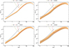Fig. 2. SGWB as detected using weakly hyperbolic encounters. The shaded regions show the SGWB and are produced from Eq. (46), where we set ri in two sets of ranges. The small range varies from {0.03 pc, 0.53 pc}, and the larger range varies from {0.03 pc, 9.03 pc}. In both cases, the eccentricity covers the range of }eimin,eimin + 4 × 10−9{. For the top-left plot, we set Ntot = 106, Rgc = 10 pc (see case 1 in the text for more details.); for the top-right plot, we set Ntot = 5 × 105, Rgc = 10 pc (see case 2 for more details); for the bottom-left plot, we set Ntot = 106, Rgc = 15 pc (see case 3 for more details); for the bottom- right plot, we set Ntot = 5 × 105, Rgc = 15 pc (see case 4 for more details). In all four cases, we integrate up to redshift z = 5. The gray region shows the case for the small ri and the orange region shows the case for the larger ri. Moreover, ET, CE, and DECIGO curves correspond to the sensitivity of the Einstein Telescope (Punturo et al. 2010), the Cosmic Explorer (Evans et al. 2021), and the Deci-hertz Interferometer Gravitational-wave Observatory (Hou et al. 2021) detectors, respectively, for one year of observation (Thrane & Romano 2013).

4.2. Total contribution to the SGWB from weakly hyperbolic encounters

Here, we present the total contribution to the SGWB from all the previous cases. In particular, n_co(z) is the same as was defined in the previous section; we let r_i vary in the whole range of }r_imin,r_imax = {=} 0.03pc,9.03pc{, and we set the same range for the eccentricity as above: }e_imin,e_imax {=}e_imin,e_imin + 4 × 10⁻⁹{. In Sect. 4.1, we set N^tot and R_gc for each case, thus fixing the virial velocity (51). However, for the total contribution of SGWB, we directly vary the virial velocity in the range 5 km s⁻¹ ≤ v_i ≤ 18 km s⁻¹. The resulting Fig. 3 shows the SGWB for the mass ranges 17 M_⊙ ≲ m₁ ≤ 55 M_⊙ and 5 M_⊙ ≲ m₂ ≤ 25 M_⊙.

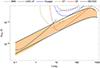Fig. 3. Total contribution to the SGWB from weakly hyperbolic encounters (orange area). In this plot, the virial velocity varies within 5 km s−1 ≤ vi ≤ 18  km s−1. The black lines around the orange area show the fitted curves for this SGWB; the bottom line represents the pessimistic scenario, while the top line is the optimistic scenario (see Sect. 4.2 for more details). Moreover, BNS, LIGO-A+, and Voyager curves correspond to the energy density of GW background of the binary neutron star (Abbott et al. 2023), and the sensitivity curves of the Advanced Laser Interferometer Gravitational-wave Observatory (Mishra et al. 2010), and the Voyager (Abbott et al. 2017; Sathyaprakash et al. 2019; see also (LIGO Scientific Collaboration et al. 2021)) detectors respectively for one year of observations.

In order to provide a reference SGWB for hyperbolic encounters, which could be compared with other SGWB from other GW sources or other GW detectors, we provide a fitted analytical expression for the Ω_GW(f) we find. Namely, from Fig. 3, we note that the plot follows a power law with a peak; we aim to fit this plot using the expression below:

$$\begin{array}{c}\hfill {\mathrm{\Omega }}_{\mathrm{GW}}(f)=a_0(1+\sum _{i=1}^{i_{\max }}{a}_i{f}^i)f^n.\end{array}$$(52)

We perform two fits, one for the maxima Ω_GW(f) of the orange area for each frequency in Fig. 3, which we refer to as the optimistic scenario, and one for the minima Ω_GW(f) of the orange area for each frequency, which we refer to as the pessimistic scenario. In the optimistic scenario, we fit the SGWB using i_max = 3, while for the pessimistic scenario, we use up to i_max = 6. In Table 1, we provide the fitting parameters for both scenarios.

5. Discussion

In this work, we studied the SGWB from hyperbolic encounters inside bound compact clusters. Specifically, we investigate weakly hyperbolic encounters with eccentricities close to one, and compute the energy density of the SGWB. By considering some assumptions, given in Sect. 3, we determine the energy density GW spectrum for a collection of hyperbolic encounters.

In Sect. 4, we present our findings and compare them with the sensitivity curves of GW detectors. First, to obtain insight into how certain parameters affect the spectra, we examine different scenarios. We consider two main cases: weakly hyperbolic encounters that occur close to the core of clusters and encounters starting from a radius close to the core out to a radius near the edge of a cluster. As shown in Sect. 4, in both cases, the SGWB from these encounters can be detected mainly by the Cosmic Explorer GW detector. However, the detectability of these spectra depends on the virial velocity and the total mass of the system. By observing the different scenarios, we find the following trends:

• As we accumulate more encounters, namely by considering more encounters from the core to the edge of the cluster, the chance of detectability increases.

• The chance of detectability increases by increasing the total mass M of the system.

• Decreasing the virial velocity increases the chance of detectability.

Having these trends in mind, we provide a total contribution of SGWB from the weakly hyperbolic encounters, where we accumulate all cases and present an analytical expression for the most optimistic and pessimistic scenarios, respectively. We conclude that the SGWB from the weakly hyperbolic encounters appears to be detectable mainly by the Cosmic Explorer and DECIGO detectors, and a marginal detection may be possible with the Einstein Telescope.

Acknowledgments

MK, S. Mukherjee, and GLG have been supported by the fellowship Lumina Quaeruntur No. LQ100032102 of the Czech Academy of Sciences. S. Mukherjee is also thankful to the Inspire Faculty Grant DST/INSPIRE/04/2022/001332, DST, Government of India, for support. Moreover, S. Mukherjee and S. Mitra are grateful to DST, Government of India, for support under the Swarnajayanti Fellowship scheme. Finally, we would like to thank Sachiko Kuroyanagi for her advisement and remarks.

References

Appendix A: Hyperbolic motion

For a hyperbolic motion with a given semi-major axis a_c and semi-minor axis b_c whose focus lies at (h, 0), we have the equation

$$\begin{array}{c}\hfill \frac{{(x-h)}^2}{{a_c}^2}-\frac{y^2}{{b_c}^2}=1.\end{array}$$(A.1)

By setting h = a_ce, where e is the eccentricity defined as $e=\sqrt{1+{(b_c/a_c)}^2}$, and using the transformation

$$\begin{array}{c}\hfill x=rcos(\varphi -{\varphi }_0),y=rsin(\varphi -{\varphi }_0),\end{array}$$(A.2)

the hyperbola (A.1) can be written in polar coordinates as

$$\begin{array}{c}\hfill r=\frac{p}{1+ecos(\varphi -{\varphi }_0)},\end{array}$$(A.3)

where p is the semilatus rectum given by $p=b_c{}^2/a_c=a_c(e^2-1)$.

By setting a_c = a/α and $b_c=b/\sqrt{\alpha }$, we arrive at

$$\begin{array}{cc}\hfill e& =\sqrt{1+\frac{b^2}{a^2}\alpha },\hfill \end{array}$$(A.4)

$$\begin{array}{cc}\hfill p& =\frac{b^2}{a}=\frac{a}{\alpha }(e^2-1),\hfill \end{array}$$(A.5)

$$\begin{array}{cc}\hfill r& =\frac{a(e^2-1)}{\alpha (1+ecos(\varphi -{\varphi }_0))}.\hfill \end{array}$$(A.6)

Thus, the trajectory given in Sect. 2.1 is actually a part of the hyperbola (A.1), where h = a_ce, a_c = a/α, and $b_c=b/\sqrt{\alpha }$.

Appendix B: Derivation of the FT

In section 2.3, we apply the FT to Eqs. (21)-(24) to derive the power radiation in the frequency domain, i.e., Eq. (25). In this section, we present the details of this derivation.

As Eqs. (21)- (24) contain sinhnξ and coshnξ, to derive the FT of these equations we need to determine $\widehat{sinhn\xi }$ and $\widehat{coshn\xi }$. Following Gröbner et al. (2020), one can get the following FTs:

$$\begin{array}{cc}\hfill \widehat{sinhn\xi }& =\frac{n}{i\omega }{e}^{\nu \pi /2}{e}^{-n\pi i/2}[K_{i\nu +n}(\nu e)+e^{i\pi n}{K}_{i\nu -n}(\nu e)],\hfill \end{array}$$(B.1)

$$\begin{array}{cc}\hfill \widehat{coshn\xi }& =\frac{n}{i\omega }{e}^{\nu \pi /2}{e}^{-n\pi i/2}[K_{i\nu +n}(\nu e)-e^{i\pi n}{K}_{i\nu -n}(\nu e)],\hfill \end{array}$$(B.2)

where ν = ω/ω₀ and

$$\begin{array}{c}\hfill K_{\alpha }(x)=\frac{1}{2}{\mathit{e}}^{\alpha \pi i/2}{\int }_{-\infty }^{+\infty }{\mathit{e}}^{\alpha \xi -ixsinh\xi }d\xi \end{array}$$(B.3)

is the modified Bessel function of the second kind. Consequently, for n = 1 and n = 2 Eqs. (B.1) and (B.2) reduce to

$$\begin{array}{cc}\hfill \widehat{sinh\xi }& =-\frac{2i}{\omega e}{\mathit{e}}^{\nu \pi /2}{K}_{i\nu }(\nu e),\hfill \end{array}$$(B.4)

$$\begin{array}{cc}\hfill \widehat{cosh\xi }& =\frac{2}{\omega }{\mathit{e}}^{\nu \pi /2}{K}_{i\nu }^{\prime }(\nu e),\hfill \end{array}$$(B.5)

$$\begin{array}{cc}\hfill \widehat{sinh2\xi }& =-\frac{2}{i\omega }{\mathit{e}}^{\nu \pi /2}((2-\frac{4}{e^2})K_{i\nu }(\nu e)-\frac{4}{\nu e}{K}_{\nu e}^{\prime }(\nu e)),\hfill \end{array}$$(B.6)

$$\begin{array}{cc}\hfill \widehat{cosh2\xi }& =\frac{8}{e\omega }{\mathit{e}}^{\nu \pi /2}(K_{i\nu }^{\prime }(\nu e)-\frac{1}{\nu e}{K}_{i\nu }(\nu e)),\hfill \end{array}$$(B.7)

where

$$\begin{array}{c}\hfill K_{\alpha }^{\prime }(x)=-\frac{1}{2}[K_{\alpha -1}(x)+K_{\alpha +1}(x)].\end{array}$$(B.8)

Now, by applying the transformation (Arfken et al. 2011)

$$\begin{array}{c}\hfill K_{\alpha }(x)=\frac{\pi }{2}{i}^{\alpha +1}{H}_{\alpha }^{(1)}(ix),\end{array}$$(B.9)

where $H_{\alpha }^{(1)}(ix)$ is the Hankel function, we arrive at

$$\begin{array}{cc}\hfill \widehat{sinh\xi }& =\frac{\pi }{\omega e}{H}_{i\nu }^{(1)}(i\nu e),\hfill \end{array}$$(B.10)

$$\begin{array}{cc}\hfill \widehat{cosh\xi }& =-\frac{\pi }{\omega }{H}_{i\nu }^{(1{)}^{\prime }}(i\nu e),\hfill \end{array}$$(B.11)

$$\begin{array}{cc}\hfill \widehat{sinh2\xi }& =\frac{\pi }{\omega }((\frac{4}{e^2}-2)H_{i\nu }^{(1)}(i\nu e)+\frac{4i}{\nu e}{H}_{i\nu }^{(1{)}^{\prime }}(i\nu e)),\hfill \end{array}$$(B.12)

$$\begin{array}{cc}\hfill \widehat{cosh2\xi }& =-\frac{\pi }{\omega }(\frac{4i}{\nu e^2}{H}_{i\nu }^{(1)}(i\nu e)+\frac{4}{e}{H}_{i\nu }^{(1{)}^{\prime }}(i\nu e)),\hfill \end{array}$$(B.13)

with

$$\begin{array}{c}\hfill H_{\alpha }^{(1{)}^{\prime }}(x)=\frac{1}{2}[H_{\alpha -1}^{(1)}(x)-H_{\alpha +1}^{(1)}(x)].\end{array}$$(B.14)

We note that Eqs. (B.10)- (B.13) are similar to the equations derived by García-Bellido & Nesseris (2018) up to a sign in sinhnξ. As the power radiation (25) contains the square of absolute values of these FTs, this sign difference does not affect the result.

All Tables

All Figures

Fig. 1. Hyperbolic trajectory of a secondary compact object of mass m2 in the gravitational field of a BH of mass m1. The secondary object is initially located at a distance ri from the primary; the initial angle between the line connecting the bodies and the initial velocity vi is θi. The motion of the secondary can be parametrized by the radial distance r(ϕ) as a function of the azimuthal angle ϕ, where ϕ lies between ri and r(ϕ). The rp is the periapsis, which is the minimum distance between the bodies, and ϕ0 is the periapsis angle, which is the angle between r(ϕ) and rp. As shown here, we define the impact parameter b as the vertical distance between the primary BH and the initial velocity of the secondary; that is, b = ri sin θi.

In the text

Fig. 2. SGWB as detected using weakly hyperbolic encounters. The shaded regions show the SGWB and are produced from Eq. (46), where we set ri in two sets of ranges. The small range varies from {0.03 pc, 0.53 pc}, and the larger range varies from {0.03 pc, 9.03 pc}. In both cases, the eccentricity covers the range of }eimin,eimin + 4 × 10−9{. For the top-left plot, we set Ntot = 106, Rgc = 10 pc (see case 1 in the text for more details.); for the top-right plot, we set Ntot = 5 × 105, Rgc = 10 pc (see case 2 for more details); for the bottom-left plot, we set Ntot = 106, Rgc = 15 pc (see case 3 for more details); for the bottom- right plot, we set Ntot = 5 × 105, Rgc = 15 pc (see case 4 for more details). In all four cases, we integrate up to redshift z = 5. The gray region shows the case for the small ri and the orange region shows the case for the larger ri. Moreover, ET, CE, and DECIGO curves correspond to the sensitivity of the Einstein Telescope (Punturo et al. 2010), the Cosmic Explorer (Evans et al. 2021), and the Deci-hertz Interferometer Gravitational-wave Observatory (Hou et al. 2021) detectors, respectively, for one year of observation (Thrane & Romano 2013).

In the text

Fig. 3. Total contribution to the SGWB from weakly hyperbolic encounters (orange area). In this plot, the virial velocity varies within 5 km s−1 ≤ vi ≤ 18  km s−1. The black lines around the orange area show the fitted curves for this SGWB; the bottom line represents the pessimistic scenario, while the top line is the optimistic scenario (see Sect. 4.2 for more details). Moreover, BNS, LIGO-A+, and Voyager curves correspond to the energy density of GW background of the binary neutron star (Abbott et al. 2023), and the sensitivity curves of the Advanced Laser Interferometer Gravitational-wave Observatory (Mishra et al. 2010), and the Voyager (Abbott et al. 2017; Sathyaprakash et al. 2019; see also (LIGO Scientific Collaboration et al. 2021)) detectors respectively for one year of observations.

In the text

References

- Abbott, B. P., Abbott, R., Abbott, T. D., et al. 2017, Class. Quant. Grav., 34, 044001 [NASA ADS] [CrossRef] [Google Scholar]
- Abbott, B. P., Abbott, R., Abbott, T. D., et al. 2019, Phys. Rev. X, 9, 031040 [Google Scholar]
- Abbott, R., Abbott, T. D., Abraham, S., et al. 2021, Phys. Rev. X, 11, 021053 [Google Scholar]
- Abbott, R., Abbott, T. D., Acernese, F., et al. 2023, Phys. Rev. X, 13, 011048 [NASA ADS] [Google Scholar]
- Afzal, A., Agazie, G., Anumarlapudi, A., et al. 2023, ApJ, 951, L11 [NASA ADS] [CrossRef] [Google Scholar]
- Agazie, G., Anumarlapudi, A., Archibald, A. M., et al. 2023, ApJ, 952, L37 [NASA ADS] [CrossRef] [Google Scholar]
- Amaro-Seoane, P., Audley, H., Babak, S., et al. 2017, ArXiv eprints [arXiv:1702.00786] [Google Scholar]
- Antoniadis, J., Arumugam, P., Arumugam, S., et al. 2024, A&A, in press, https://doi.org/10.1051/0004-6361/202347433 [Google Scholar]
- Arca Sedda, M. 2020, Commun. Phys., 3, 43 [CrossRef] [Google Scholar]
- Arfken, G. B., Weber, H. J., & Harris, F. E. 2011, in Mathematical Methods for Physicists, 7th edn. (Academic Press) [Google Scholar]
- Boileau, G., Lamberts, A., Christensen, N., Cornish, N. J., & Meyer, R. 2021, ArXiv eprints [arXiv:2105.06793] [Google Scholar]
- Cho, G., Gopakumar, A., Haney, M., & Lee, H. M. 2018, Phys. Rev. D, 98, 024039 [NASA ADS] [CrossRef] [Google Scholar]
- Chowdhuri, A., Singh, R. K., Kangsabanik, K., & Bhattacharyya, A. 2023, ArXiv eprints [arXiv:2306.11787] [Google Scholar]
- De Vittori, L., Jetzer, P., & Klein, A. 2012, Phys. Rev. D, 86, 044017 [NASA ADS] [CrossRef] [Google Scholar]
- Dymnikova, I. G., Popov, A. K., & Zentsova, A. S. 1982, Astrophys. Space Sci., 85, 231 [CrossRef] [Google Scholar]
- Evans, M., Adhikari, R. X., Afle, C., et al. 2021, ArXiv eprints [arXiv:2109.09882] [Google Scholar]
- García-Bellido, J., & Nesseris, S. 2018, Phys. Dark Univ., 21, 61 [CrossRef] [Google Scholar]
- García-Bellido, J., Jaraba, S., & Kuroyanagi, S. 2022, Phys. Dark Univ., 36, 101009 [Google Scholar]
- Gröbner, M., Jetzer, P., Haney, M., Tiwari, S., & Ishibashi, W. 2020, CQG, 37, 067002 [CrossRef] [Google Scholar]
- Hou, S., Li, P., Yu, H., et al. 2021, Phys. Rev. D, 103, 044005 [CrossRef] [Google Scholar]
- Jakobsen, G. U., Mogull, G., Plefka, J., & Steinhoff, J. 2021, Phys. Rev. Lett., 126, 201103 [NASA ADS] [CrossRef] [Google Scholar]
- Kocsis, B., Gáspár, M. E., & Márka, S. 2006, ApJ, 648, 411 [NASA ADS] [CrossRef] [Google Scholar]
- Kremer, K., Ye, C. S., Rui, N. Z., et al. 2020, ApJS, 247, 48 [NASA ADS] [CrossRef] [Google Scholar]
- LIGO Scientific Collaboration, Virgo Collaboration, & KAGRA Collaboration 2021, in GWTC-3: Compact Binary Coalescences Observed by LIGO and Virgo During the Second Part of the Third Observing Run, https://dcc.ligo.org/LIGO-P2000318/public [Google Scholar]
- LIGO Scientific Collaboration, Virgo Collaboration, & KAGRA Collaboration 2023, Phys. Rev. X, 13, 041039 [Google Scholar]
- Longair, M. S. 2023, Galaxy Formation (Berlin, Heidelberg: Springer) [CrossRef] [Google Scholar]
- Maggiore, M. 2007, Gravitational Waves. Vol. 1: Theory and Experiments (Oxford University Press) [Google Scholar]
- Maggiore, M. 2018, Gravitational Waves: Volume 2: Astrophysics and Cosmology (Oxford University Press) [Google Scholar]
- Maggiore, M., Van Den Broeck, C., Bartolo, N., et al. 2020, J. Cosmol. Astropart. Phys., 2020, 050 [CrossRef] [Google Scholar]
- Martinovic, K., Meyers, P. M., Sakellariadou, M., & Christensen, N. 2021, Phys. Rev. D, 103, 043023 [NASA ADS] [CrossRef] [Google Scholar]
- Mishra, C. K., Arun, K. G., Iyer, B. R., & Sathyaprakash, B. S. 2010, Phys. Rev. D, 82, 064010 [NASA ADS] [CrossRef] [Google Scholar]
- Morrás, G., García-Bellido, J., & Nesseris, S. 2022, Phys. Dark Univ., 35, 100932 [CrossRef] [Google Scholar]
- Mukherjee, S., Mitra, S., & Chatterjee, S. 2021, MNRAS, 508, 5064 [NASA ADS] [CrossRef] [Google Scholar]
- Punturo, M., Abernathy, M., Acernese, F., et al. 2010, Class. Quant. Grav., 27, 084007 [NASA ADS] [CrossRef] [Google Scholar]
- Roskill, A., Caldarola, M., Kuroyanagi, S., & Nesseris, S. 2023, ArXiv eprints [arXiv:2310.07439] [Google Scholar]
- Saketh, M. V. S., Vines, J., Steinhoff, J., & Buonanno, A. 2022, Phys. Rev. Res., 4, 013127 [NASA ADS] [CrossRef] [Google Scholar]
- Sathyaprakash, B., Bailes, M., Kasliwal, M. M., et al. 2019, BAAS, 51, 276 [NASA ADS] [Google Scholar]
- Thrane, E., & Romano, J. D. 2013, Phys. Rev. D, 88, 124032 [NASA ADS] [CrossRef] [Google Scholar]
- Vines, J., Steinhoff, J., & Buonanno, A. 2019, Phys. Rev. D, 99, 064054 [NASA ADS] [CrossRef] [Google Scholar]
- Zhu, X.-J., Howell, E. J., Blair, D. G., & Zhu, Z.-H. 2013, MNRAS, 431, 882 [NASA ADS] [CrossRef] [Google Scholar]