| Issue |
A&A
Volume 684, April 2024
|
|
|---|---|---|
| Article Number | A116 | |
| Number of page(s) | 16 | |
| Section | Planets and planetary systems | |
| DOI | https://doi.org/10.1051/0004-6361/202348042 | |
| Published online | 10 April 2024 | |
The GAPS Programme at TNG
LIII. New insights on the peculiar XO-2 system★,★★
1
Department of Physics and Astronomy, University of Padova,
Vicolo dell’Osservatorio 2,
35122
Padova, Italy
e-mail: This email address is being protected from spambots. You need JavaScript enabled to view it.
2
INAF, Astrophysical Observatory of Padova,
Vicolo dell’Osservatorio 5,
35122
Padova, Italy
3
INAF, Astronomical Observatory of Rome,
Via Frascati 33,
00178
Monte Porzio Catone (RM), Italy
4
INAF, Astrophysical Observatory of Turin,
Via Osservatorio 20,
10025
Pino Torinese (TO), Italy
5
Department of Physics and Astronomy, University of Padova,
via Marzolo 8,
35131
Padova, Italy
6
INAF, Astrophysical Observatory of Catania,
Via S. Sofia 78,
95123
Catania, Italy
7
INAF, Astronomical Observatory of Palermo,
Piazza del Parlamento 1,
90134
Palermo, Italy
8
INAF, Astronomical Observatory of Trieste,
via Tiepolo 11,
34143
Trieste, Italy
9
Fundación Galileo Galilei – INAF,
Rambla José Ana Fernández Pérez 7,
38712
Breña Baja, Tenerife, Spain
10
INAF, Astronomical Observatory of Brera,
Via E. Bianchi 46,
23807
Merate (LC), Italy
11
INAF, Astrophysical Observatory of Arcetri,
Largo Enrico Fermi 5,
50125
Firenze, Italy
Received:
22
September
2023
Accepted:
12
January
2024
Abstract
Context. Planets in binary systems are a fascinating and yet poorly understood phenomenon. Since there are only a few known large-separation systems in which both components host planets, characterizing them is a key target for planetary science.
Aims. In this paper, we aim to carry out an exhaustive analysis of the interesting XO-2 system, where one component (XO-2N) appears to be a system with only one planet, while the other (XO-2S) has at least three planets.
Methods. Over the last 9 yr, we have collected 39 spectra of XO-2N and 106 spectra of XO-2S with the High Accuracy Radial velocity Planet Searcher for the Northern emisphere (HARPS-N) in the framework of the Global Architecture of Planetary Systems (GAPS) project, from which we derived precise radial velocity (RV) and activity indicator measurements. Additional spectroscopic data from the High Resolution Echelle Spectrometer (HIRES) and from the High Dispersion Spectrograph (HDS), and the older HARPS-N data presented in previous papers, have also been used to increase the total time span. We also used photometric data from TESS to search for potential transits that have not been detected yet. For our analysis, we mainly used PyORBIT, an advanced Python tool for the Bayesian analysis of RVs, activity indicators, and light curves.
Results. We found evidence for an additional long-period planet around XO-2S and characterized the activity cycle likely responsible for the long-term RV trend noticed for XO-2N. The new candidate is an example of a Jovian analog with m sin i ~ 3.7 MJ, a ~ 5.5 au, and e = 0.09. We also analyzed the stability and detection limits to get some hints about the possible presence of additional planets. Our results show that the planetary system of XO-2S is at least one order of magnitude more massive than that of XO-2N. The implications of these findings for the interpretation of the previously known abundance difference between components are also discussed.
Key words: techniques: radial velocities / planets and satellites: detection / binaries: visual / stars: individual: XO-2SXO-2N / stars: solar-type
The individual HARPS-N RV time series are available at the CDS via anonymous ftp to cdsarc.cds.unistra.fr (130.79.128.5) or via https://cdsarc.cds.unistra.fr/viz-bin/cat/J/A+A/684/A116
Based on observations made with the Italian Telescopio Nazionale Galileo (TNG), operated on the island of La Palma by the INAF – Fundación Galileo Galilei at the Roque de Los Muchachos Observatory of the Instituto de Astrofísica de Canarias (IAC).
© The Authors 2024
 Open Access article, published by EDP Sciences, under the terms of the Creative Commons Attribution License (https://creativecommons.org/licenses/by/4.0), which permits unrestricted use, distribution, and reproduction in any medium, provided the original work is properly cited.
This article is published in open access under the Subscribe to Open model. This email address is being protected from spambots. You need JavaScript enabled to view it. to support open access publication.
1 Introduction
In recent years, the number of discovered exoplanets has constantly increased thanks to the great effort of the astronomical community and technological advancements. In this context, a research field that has not greatly advanced yet is that of planetary systems around binary stars. These are typically more difficult to study but they can yield interesting information regarding the formation and evolution processes. This is important because binaries represent about one-third of all the stars in our Galaxy (e.g., Raghavan et al. 2010), and therefore a complete comprehension of planetary systems requires the study of these objects. Planets orbiting around one component of a binary system are called S types, and several works have tried to determine how and when the stellar companion can affect them. As reported by Eggenberger & Udry (2010), S-type planets do indeed display different properties than those around a single star. This is mainly driven by the dynamical interactions with the companion, in particular for binaries closer than 100 au. The difficulty in detecting and characterizing planets in close binaries often leads to their exclusion from planet search surveys. On the other hand, wide binaries are more favorable targets and can be taken into consideration for a proper analysis of the population of planets in binary systems.
Binary systems in which both stars host planets are of particular interest as it is possible to carry out comparative studies since the two stars likely formed from the same cloud (i.e., the same chemical composition and age) and experienced similar dynamical perturbations. Very few such cases of double-planet hosts are currently known: HD 20781 and HD 20782 (Jones et al. 2006; Udry et al. 2019), WASP-94 (Neveu-Van Malle et al. 2014), Kepler-132 (Lissauer et al. 2014), and XO-2, the first binary system for which both components were found to host planets, which is the target of this paper. In this context, the XO-2 system is of great interest as it presents unique features that make it an important target. In particular, it includes two widely separated stars XO-2S and XO-2N (separation 31″, projected separation ~4600 au) that are almost identical to each other and to the Sun, except that they both have metallicities more than twice that of the Sun. Burke et al. (2007) discovered a transiting hot Jupiter around XO-2N, while Desidera et al. (2014) identified two planetary companions around XO-2S, a warm Saturn-like and a temperate Jupiter-like one, through radial velocity (RV) monitoring. Long-term RV trends were seen for both components (Damasso et al. 2015) and the one of XO-2N may be due to an activity cycle. Further characterization of the transiting planet showed a well-aligned configuration through the Rossiter-McLaughlin effect (Narita et al. 2011; Damasso et al. 2015). The photometric variability and the stellar activity were studied by Zellem et al. (2015) and Damasso et al. (2015), with tentative measurements of the rotation period of XO-2N and an indication that it is slightly more active, possibly because of interactions with its very close-in planet. Independent studies on the chemical abundances of the two components showed that XO-2N is also slightly more metal rich than XO-2S (Teske et al. 2015, Biazzo et al. 2015; Ramírez et al. 2015) with indications of a dependence of the abundance difference from the condensation temperature. This is interesting because visual binaries are expected to form from the same cloud, and they should thus have the same composition. In the first case, the “original” composition is that of the S component, and the N star has been enriched because the inward migration of planet b caused a potential companion to collide with the star, releasing rocky material in the stellar atmosphere. In the other scenario, XO-2S is instead depleted of metals with respect to the original composition because its heavy elements are locked into the planetary cores and therefore the star accreted (relatively) metal-depleted gas in the final stages of formation. In order to shed further light on this system of special interest, the first step is to fully characterize the planetary systems of both stars, in particular by analyzing the previously mentioned long-term RV trends and understanding their origin. This was accomplished with the continuation of the RV monitoring of both components for an additional 9 yr with respect to Damasso et al. (2015). We also took advantage of the available TESS data to look for transits of XO-2S b and c, and for stellar characterization. Section 2 describes the new observations, the archive data, and the adopted data analysis procedures. In Sect. 3, we briefly describe the stellar parameters adopted in our analysis. In Sects. 4 and 5 we present the results for XO-2S and XO-2N, respectively. In Sect. 6, the implications of our findings are discussed. In Sect. 7 we summarize our conclusions.
2 Observations and data analysis
2.1 High resolution spectroscopy
2.1.1 HARPS-N spectra
After the studies of the system by Desidera et al. (2014) and Damasso et al. (2015), spectroscopic monitoring of XO-2S and XO-2N was continued in the framework of the General Architecture of Planetary Systems (GAPS) program (Covino et al. 2013) to properly characterize the long-term trends observed for both components. Observations were performed with the High Accuracy Radial velocity Planet Searcher for the Northern emisphere (HARPS-N) spectrograph at the Telescopio Nazionale Galileo (TNG, Cosentino et al. 2012), with a typical integration time of 900 s for each component. For XO-2N, we collected 39 spectra between October 6, 2014, and May 10, 2023. For XO-2S, we gathered 106 spectra from September 10, 2014, to April 5, 2023.
Radial velocities (RVs) were obtained with the HARPS-N pipeline using the online tool YABI1, using a K5 mask for the cross-correlation function (CCF). The pipeline provides additional indicators used in our analysis such as the Bisector Inverse Span (BIS) and the full width at half maximum (FWHM) of the CCF. We also exploited the YABI tool, with the procedure based on Lovis et al. (2011), to measure the S Index, calibrated onto the Mount Wilson scale, and the chromospheric activity index log R′HK. In addition, we derived the Hα and NaI activity indicators, both extracted from the spectra using the Python tool ACTIN 22 (Gomes da Silva et al. 2018, 2021).
The basic properties of the RV time series are summarized in Table 1, while the individual HARPS-N RV time series are available at the CDS. For XO-2N, we found a few outliers that we had to remove. In particular, we removed the spectrum taken on 18 October 2016 because it was contaminated by the Sun, the one taken on 06 January 2013 because the integration time was 1 s, and finally, the one taken on 27 December 2012 because of a technical issue.
2.1.2 Archive and literature data
As for the RVs, there are data available for XO-2N taken with the High Resolution Echelle Spectrometer (HIRES) by Butler et al. (2017), the High Dispersion Spectrograph (HDS) by Narita et al. (2011), and with the Spectrographe pour l’Observation des Phénomènes des Intérieurs stellaires et des Exoplanètes (SOPHIE)3. Additionally, there are the original data taken by Burke et al. (2007) with the High-Resolution Spectrograph (HRS) on the McDonald Observatory 11-m Hobby-Eberly Telescope (HET) for both stars but we did not include them because of their low quality compared to the other sets. After a few tests, we eliminated the SOPHIE data from our analysis because of their lower precision (the resulting RV jitter was ~38 m s−1, while for the other datasets it was <10 m s−1). The HIRES data include values of the SMW activity index, while the HDS data do not. The authors state that their S-index values are already calibrated in the Mount Wilson scale, so they can be directly compared with the HARPS-N ones. No error bars are reported for the HIRES SMW. Therefore, we took those points that were grouped within a few days and calculated the standard deviation. After doing so for two clusters of points, we made the average of the sigmas and used the resulting value as the error bar for the whole set. This implies that the obtained error bars are likely an overestimate of the instrumental error and might be affected by a rotational modulation. Of the HDS RV data set, we only kept those points that were not affected by the Rossiter-McLaughlin effect (Rossiter 1924; McLaughlin 1924).
The properties of the datasets are shown in Table 1.
Properties of the datasets.
2.2 Photometric data from TESS
Our targets have been observed with the Transiting Exoplanet Survey Satellite (TESS, Ricker et al. 2015) in sectors 20, 47, and 60 in a 2-min cadence. In the TESS catalog, the two stars are labeled as TIC 356473034 (XO-2N) and TIC 356473029 (XO-2S). The light curves are obtained with the pipeline developed by the Science Processing Operations Centre (SPOC, Jenkins et al. 2016). The Simple Aperture Photometry (SAP) light curves have been downloaded with the lightkurve Python package (Lightkurve Collaboration 2018). We decided to exploit the XO-2S data to check whether we can reveal the transits of XO-2S b and c, and the XO-2N data to try to constrain the rotation period of this component. The main problem is that the two stars are partially blended, and therefore the analysis requires thorough care. In particular, the transits of the planets of XO-2S might be diluted by the light of XO-2N.
2.3 Data analysis tools
2.3.1 Periodograms
We extracted periodograms using the astropy Python package. For XO-2N we first extracted the Generalized Lomb-Scargle periodogram (GLS, Zechmeister & Kürster 2009) of the HARPS-N data alone to estimate the offset and subtract it before doing the same with the complete RV time series. We did not follow the same procedure for the HIRES and HDS sets because there are too few points and such a process could lead to the determination of an inaccurate offset. This issue is not present for XO-2S as only HARPS-N data are available for this target. In all cases, the reported False Alarm Probabilities (FAPs) have been calculated with the bootstrap method.
2.3.2 Orbital fit
For the data analysis in this work, we used the 9.1 version of the Python tool PyORBIT4 (Malavolta et al. 2016, 2018), a package for the Markov chain Monte Carlo (MCMC) modeling of RVs, activity indicators, and light curves. In particular, it is based on the combination of the optimization algorithm PyDE5 (Storn & Price 1997) and the affine invariant MCMC sampler emcee6 (Foreman-Mackey et al. 2013). For the analysis of stellar activity data, we resorted to Gaussian Process (GP) regression with a quasi-periodic kernel as in the last years this technique has proven to be quite effective for this purpose (e.g., Grunblatt et al. 2015). In this context, the hyperparameter h can be seen as the amplitude of the activity contribution to the RV signal, while θ is the period. In all cases, we ran the algorithm for 200 000 steps with a burn-in parameter of 50 000. For both RVs and activity indices, we introduced separate offset and jitter terms for HIRES, HDS, and HARPS-N data, respectively. We performed several fits for each target, selecting the best ones based on the Bayesian Information Criterion (BIC) value (Schwarz 1978). In addition, we also considered the Gelman-Rubin diagnostic (Gelman & Rubin 1992) to check for convergence of the parameters. In all cases, the reference time is BJD = 2458 842.
2.3.3 Light curve analysis
Before analyzing the TESS light curves with PyORBIT to search the signals corresponding to the planets known from RVs, we made some preparatory steps. First, we downloaded the SAP light curves, removing NaNs and outliers above 4 σ. As previously mentioned, the two components of the binary system are blended and, therefore, we estimated the dilution factor for XO-2S as described in Sect. 2.2.2 of Mantovan et al. (2022), obtaining a value of 0.376 ± 0.003 used to further correct our data and remove the contribution of the N component. Finally, we masked and removed the transits of XO-2N b. The light curves are shown in Fig. 1.
3 Stellar parameters
The two stars of this binary system are both G9V main sequence stars at a distance of ~150 pc. The two components have a separation of ~31 arcsec, implying a physical distance of ~4600 au. They have been thoroughly analyzed in many papers (Desidera et al. 2014; Damasso et al. 2015; Biazzo et al. 2015; Teske et al. 2015; Zellem et al. 2015) and the recent results from Gaia DR3 yield a trigonometric distance basically identical to the previously adopted one. Therefore we did not perform any additional analysis to retrieve their physical parameters. In this work, we adopted the values reported in Damasso et al. (2015) for our analysis. In particular, the masses and the radii are taken from their Table 2 (for XO-2N, we used the values marked with number 2 in the notes), while the other parameters are taken from the differential analysis results in Table 3 as this method has proven to be very effective in this case (see the original paper for an in-depth discussion). Such values are shown in Table 2.
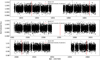 |
Fig. 1 TESS light curves of XO-2S after removing outliers above 4 σ, normalizing, correcting for dilution, and removing the transits of XO-2N b. The red bars indicate the predicted transits for planet b from RV results, as explained in Sect. 4.4. |
Physical stellar parameters as derived in Damasso et al. (2015).
4 XO-2S: Evidence for a new Jupiter-analog planet
4.1 Previous works
The two planets in the XO-2S system were announced by Desidera et al. (2014). Planet b is a warm Saturn-like planet with P ~ 18 d and m sin i ~ 0.26 MJ, while planet c is a temperate Jovian with P ~ 126 d and m sin i ~ 1.37 MJ. A long-term RV trend was also noticed. In that work and also in Damasso et al. (2015) it has been noted that activity does not seem to contribute to the RV signal. Nevertheless, since in the last 9 yr we have expanded our data set with 106 more spectra, we considered its inclusion in the modeling of the time series.
4.2 Periodogram analysis of XO-2S
The GLS computed from the RVs of XO-2S reveals a clear peak corresponding to planet c. The residuals show a significant peak at ~4500 d, as shown in Fig. 2, revealing the presence of a potential additional planet. The other significant peak at larger frequencies corresponds to the signal of planet b. The periodogram of the activity index SMW time series shows a peak at 3846 d with FAP In spite of that, we included this activity index in our fit to evaluate the contribution of stellar activity to the RV signal. We computed the GLS of two more activity indicators, the BIS and the FWHM of the CCF, but did not retrieve any information worth mentioning.
4.3 Orbital fit of XO-2S
After the periodogram analysis, we proceeded with the full orbital analysis with PyORBIT. To fully explore the parameter space, we performed the following orbital fits:
Two planets without activity: this includes the two known planets and has been used as a reference (Model 1, M1).
Three planets without activity: since there is a long-period signal, we fit it with a Keplerian (Model 2, M2).
Two planets with quasi-periodic GP: this has been done to check whether the long-term signal might be due to an activity cycle rather than an additional planet (Model 3, M3).
Three planets with quasi-periodic GP: to explore the possibility that there is an additional planet but the star also experiences an activity cycle that contributes to the RV signal (Model 4, M4).
We obtain BIC(M1) = 663.0, BIC(M2) = 22.5, BIC(M3) = 44.1, and BIC(M4) = 53.1. We consider the model selection criterium by Kass & Raftery (1995) according to which a model is strongly favored over another when ΔBIC > 10. In our cases, we have ΔBIC = 21.6, 30.6, and 640.5 in favor of M2 compared to M3, M4, and M1, respectively, and therefore conclude that there is strong evidence that Model 2 is the most convincing representation of the actual RV data. The best-fit model (Model 2) is shown in Fig. 3, while Figs. 4–6 show the Keplerian models of planet b, c, and d, respectively. The planetary parameters are shown in Table 3. As we can see in Fig. 6, unluckily our time series does not sample any minima of the signal corresponding to the third object. This implies a correlation between Kd and Pd, as shown in the corner plot in Fig. 7. Therefore, our results on md sin id are likely underestimated and should be considered as a minimum value. For this reason, we performed an additional fit including in the model two Keplerians and a quadratic trend (Model 5, M5) to see whether we could fit the data with a simple polynomial term instead of a full Keplerian curve. With this model, we obtained BIC(M5) = 171.5 and thus discarded it as unfavored. In addition, in such a model, the error bars of the orbital parameters of the known planets are 50–60% larger and the jitter term is more than twice (4.8 vs. 2.1 m s−1) compared to the 3-planets case.
In summary, we confirm the two planetary companions XO-2S b and c originally discovered by Desidera et al. (2014), with minor differences in the orbital parameters but much smaller error bars (ranging from 3 to 70% of the older value for Pb and mb sin ib, respectively), and we identified a new planetary companion, to be named XO-2S d, in a Jupiter-like orbit (a = 5.46 au, e = 0.091) with a minimum mass of 3.71 MJ. In the GLS of the RV residuals, the highest peak is at 30 d with FAP = 7.4%, thus we have no evidence for additional planets in the system with the current data set.
Planetary parameters obtained from the best-fit models.
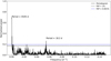 |
Fig. 2 GLS of the RV residuals of XO-2S after removing the signal corresponding to planet c. The peak at 18.2 d corresponds to planet b. |
4.4 Search for transits of XO-2S b and c in TESS data
So far, in the literature, there have been no dedicated transit searches of the two inner planets of XO-2S. For this reason, we looked for potential transit signals in the TESS light curves. Since planet b is quite close to its star (a ~ 0.13 au), the search for its transit is promising. Planet c is 3.5 times more distant; therefore, only a smaller range of inclinations would allow it to transit. We note here that, assuming a radius equal to that of Jupiter and i = 90°, the transit durations are around 6 and 11 h for the two planets.
Since our RVs results are robust and the error bars on the orbital parameters are pretty low, we used them to predict where the potential transits could occur within the TESS sectors (see, e.g., Kane 2007). The uncertainty on the transit times is calculated as
 (1)
(1)
where  is the uncertainty on the time of the first transit, σP the error on the orbital period, and n an integer indicating the number of periods passed between the reference ephemerids and the time of TESS data. Rigorously speaking, one should include the light-time effect produced by the motion of XO-2N around the barycenter of the visual binary when estimating the difference in the times of mid-transits. Nevertheless, an order of magnitude estimate shows that the amplitude of the light-time effect is on the order of 1 min over a time span of ten years, that is, it is negligible compared to the variation associated with the uncertainty of the orbital period of the planet. The values for
  and σΡ are reported in Table 3, and we used BJD = 2458 842 as reference time since it corresponds to the beginning of the TESS observations in Sector 20. In particular, we find for planet b a total of 5 potential transits at BJD = 2458 848.32, 2458 866.54, 2459 595.33, 2459941.50, and 2459 959.72, with an error of 0.4 d for Sector 60. However, the third predicted transit falls inside the TESS instrumental gap in Sector 47 (as shown in Fig. 1) and so it must not be considered. In Eq. (1), we used the error on the time of periastron passage instead of
  because we have no previous known transit. Unfortunately, none of the predicted transits for planet c fall in the range covered by the TESS data, even considering the error bar of 1 d. For the sake of completeness, we also considered the possibility that the new candidate is transiting. We calculated the predicted times of transits and the associated uncertainties using the full posterior distribution of its orbital parameters. We found that, considering the uncertainty, the predicted time of transit is at least 500 d before the beginning of Sector 20, and the next one falls almost 2400 d after the end of Sector 60. Therefore, we carried on with the analysis searching for one potentially transiting planet.
As a first step, we used the Python package transitleastsquares (Hippke & Heller 2019) to compute the Transit Least Squares (TLS) of the TESS light curves to detect any potential planetary signal. Unfortunately, we found no significant signal but proceeded with a full analysis to make sure we did not leave anything behind and, for example, a very grazing transit could perhaps remain undetected with the TLS approach. Before proceeding with the PyORBIT analysis, we estimated the limb-darkening coefficients (quadratic law) using the Python code PyLDTk (Parviainen & Aigrain 2015), based on the spectrum library by Husser et al. (2013). Using the effective temperature, log g, and metallicity reported in Table 2 for XO-2S, we obtained the values u1 = 0.4690 ± 0.0066 and u2 = 0.1119 ± 0.0198, and we set them as priors in our light curve analysis. In addition, we set the following priors: the period of the planet as obtained from the RV analysis, the transit time given by the first predicted transit, and the stellar density (0.925 ± 0.25 ρ⊙) using the mass and radius in Table 2. We also fixed the eccentricity and ω values since these are not retrieved from the light curves.
Unfortunately, our results indicate that a transit of XO-2S b is very unlikely to be present in the TESS data. In particular, we obtain an impact parameter  and a planetary radius
  . The nominal values are clearly nonphysical (the radius implies an Earth-like density for a gas giant), and the extremely large error bars are due to posterior distributions that are either almost flat (impact parameter) or peaked at very low values and then flat up until very large ones (planetary radius). Therefore, we must conclude that, at present, the evidence is that XO-2S b is non-transiting. As said before, we cannot say anything about XO-2S c and d but if their orbits are coplanar to that of planet b (or very close to it), then they are also very unlikely to transit.
As a final step, we checked the sensitivity of TESS data to the presence of planet b. In practice, we injected fake transits at the times predicted by RV results with the Python package batman (Kreidberg 2015) and tried to recover them with the TLS. We used Rp/Rs = 0.12 (corresponding to roughly Jupiter’s radius) and repeated the procedure with decreasing radii until the transit was no longer recovered significantly, that is when SED ≲ 10. For this analysis, we fixed i = 90, while also noticing that the transit condition for this planet is 88° ≤ i ≤ 92° based on its RV-derived orbital parameters. We note that, at the first step, we obtain SED = 24.9. We continued the analysis down to Rp/Rs = 0.04 (roughly Neptune’s radius), in which case we found SED = 9.5. These results indicate that, with the current TESS data, we are potentially able to detect a transiting planet slightly larger than Neptune. Since the minimum mass of XO-2S b is 0.26 MJ, we expect its radius to be ~1 RJ and this further confirms that, if it was transiting, we would be able to see it.
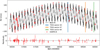 |
Fig. 3 Best-fit model (Model 2) of XO-2S. |
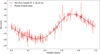 |
Fig. 4 Best-fit Keplerian model for XO-2S b (phase-folded), after removing the RV signal of the other two planets. |
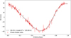 |
Fig. 5 Best-fit Keplerian model for XO-2S c (phase-folded), after removing the RV signal of the other two planets. |
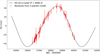 |
Fig. 6 Best-fit Keplerian model for XO-2S d, after removing the RV signal of the other two planets. |
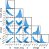 |
Fig. 7 Corner plot of the orbital parameters of the new candidate XO-2S d obtained from our analysis. |
4.5 Dynamical stability of the system
The long-term stability of the system has been tested with the chaos indicator MEGNO, the Mean Exponential Growth factor of Nearby Orbits (Cincotta & Simó 2000; Gozdziewski et al. 2001) closely related to the maximum Lyapunov exponent. It is computed by solving the variational equations of the dynamical system to evaluate the relative divergence of orbits. The value of MEGNO in the case of regular or quasi–periodic orbits is very close to 2, while for chaotic motion it increases with time. The system of three planets for the nominal values of the masses and orbital parameters given in Table 3 is stable, according to MEGNO. We increased the planets’ masses up to 10 times their nominal values, assuming the planets are coplanar (corresponding to an inclination of (i ~ 6°), but the system remains stable.
We also investigated the location of a potential additional planet on a stable orbit. We have assumed an Earth mass for this putative planet and randomly sampled its orbital elements. The semi-major axis is varied between 0.05 and 12 au while the eccentricity ranges from 0 to 0.5. Stable regions which could harbor an additional Earth-like planet are found mainly in the 1–3 au range, and beyond 9 au, as shown in Fig. 8. There are also some stable orbits corresponding to Mean Motion Resonances. If we increase the masses by a factor of 3 (Fig. 9), the prominent stable regions get smaller and the resonant orbits are no longer stable. The situation worsens if we increase the masses by a factor of 10, even though the main stable regions remain. Unfortunately, as we describe in Sect. 6.2, astrometry does not help us to rule out the low inclinations (i ~ 6°) that this hypothetical scenario implies.
As a final case, we focused on the region at a < 0.5 au, increasing the spatial sampling. Despite a few isolated stable cases, we find that most of this region is unstable, especially between the two inner planets. These results have been obtained by fixing the masses to the m sin i.
 |
Fig. 8 Stability results using the chaos indicator MEGNO (color bar on the right) for XO-2S, using the nominal values for the masses of the three planets. |
5 XO-2N: An activity cycle inducing a planetary-like signal
5.1 Previous works
XO-2N b has been discovered by Burke et al. (2007) with the transit method and an RV follow-up. It is a hot Jupiter with P = 2.6 d and Mp ~ 0.6 MJ. Damasso et al. (2015) noted the presence of a long-term trend in the RV time series and pointed out the possibility that it was caused by a magnetic cycle of the star but at the time they did not have enough data points to confirm this statement. Now, we have 39 more spectra gathered over the last 9 yr and even more accurate ephemeris for planet b thanks to TESS data (Ivshina & Winn 2022), so we analyzed this system once again to determine the nature of the additional RV signal.
5.2 Periodogram analysis of XO-2N
The periodogram of the RVs of XO-2N displays an extremely well-peaked signal at the period of planet b (~2.6 d). The GLS of the RV residuals obtained by fitting a 1-planet model without any activity contribution displays a signal at a little less than 3000 d, even though it is not particularly strong (FAP ~ 2%). A similar peak (2754 d) is found in the BIS data, even though its FAP is 25% and therefore unreliable. This is probably due to the fact that the BIS data only come from the HARPS-N data set and therefore cover a much smaller time range. A similar peak (P ~ 3600 d) is found in the SMW time series (FAP ~ 0.001%). These are shown in Fig. 10. The combination of these three results suggests the presence of a common cycle with a period of about 9–10 yr.
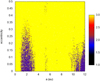 |
Fig. 9 Stability results using the chaos indicator MEGNO (color bar on the right) for XO-2S, increasing the masses of the three planets by a factor of 3 with respect to the m sin i. |
5.3 Correlation between RVs and activity indicators
Damasso et al. (2015) first noted that the long-term trend observed in the RVs of XO-2N could be due to an activity cycle. In particular, they showed that the residuals of the 1-planet model were strongly correlated with the activity index SMW (Spearman’s rank r = 0.68, FAP = 10−4). The result was obtained by selecting only the data points with a signal-to-noise ratio (S/N) ≥ 4 in the 6th spectral order, which corresponds to the part of the spectrum where the Ca II H & K lines are located. Following the same approach, we first fit the RV time series with a 1-planet model and then searched for the same correlation for different activity indices. Once again, we kept only the observations with S/N ≥ 4. For this reason, we only used HARPS-N data for this analysis because we have more control over the observations and their technical information. The parameters obtained for planet b in the orbital fit are compatible with the ones found in previous works and are shown in Table 3.
Figure 11 shows the correlations between the RVs and two activity indices, namely SMW and the BIS. As we can see, the correlation with the S-index is rather strong (r = 0.51 and p = 0.0027), even though nominally weaker than that found in Damasso et al. (2015). However, this is intrinsically more significant because it has been obtained using a larger data set over a much longer time range. The correlation with the BIS is weaker and less significant (r = 0.31 and p = 0.08), indicating that the activity signature in the RV is probably better mapped by the chromospheric features rather than photospheric ones (starspots). It is likely that the photospheric blue shift quenching is dominating the cyclic RV variations in this star, which is not particularly active, as it happens in the Sun (cf. Lanza et al. 2016). Such a quenching is indirectly mapped by the chromospheric emission because it is produced by magnetic fields that are more diffuse and weaker than those in dark starspots. Those relatively weak fields manifest themselves as faculae and are associated with a chromospheric signature. We applied the same analysis using the Hα and Na I indicators, obtaining r = 0.35 and p = 0.05 for both indices, indicating a weak correlation. Finally, we studied the correlation between RV residuals and the FWHM of the CCF. To do this, we had to remove the data points taken before March 2014 (14 spectra) because of a small defocus of the instrument, as explained in Benatti et al. (2017). With the remaining set, we obtain r = 0.54 and p = 0. 016, once again proving a correlation between RVs and the star’s activity.
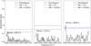 |
Fig. 10 Periodograms of XO-2N. Left panel: GLS of RV residuals of XO-2N obtained from a 1-planet model without activity. Central panel: GLS of the BIS data of XO-2N. Right panel: GLS of the SMW activity index of XO-2N. |
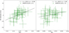 |
Fig. 11 Correlations between RV residuals and activity indicators of XO-2N. Left panel: correlation between SMW and RV residuals. Right panel: same correlation but between the BIS indicator and RV residuals. |
5.4 Rotation period
As shown in the previous section, stellar activity is clearly affecting our RVs for XO-2N. While the periodograms presented in Sect. 5.2 suggest that the most significant stellar variability is on a timescale of several years and then likely linked to an activity cycle, the investigation of the stellar rotation period is also highly relevant for a better understanding of the activity behavior of the star and to drive the most appropriate choices for the RV modeling (Sect. 5.5).
Damasso et al. (2015) tried to determine the rotation period of this star using ~800 APACHE I-band data points, finding a value of 41.6 ± 1.1 d. This is consistent with the values expected from the SMW and color values, in particular, we obtain 39.6 ± 0.6 d using the expression by Noyes et al. (1984) and 41.8 ± 0.8 using instead the formula by Mamajek & Hillenbrand (2008). On the other hand, Zellem et al. (2015) found low-amplitude brightness variations with periods of 29.9 ± 0.16 d in the 2013–2014 season and 27.34 ± 0.21 d in the 2014–2015 season. These values are incompatible with the previously mentioned results but, as the authors point out, still fall in the 29–44 range predicted by Burke et al. (2007) based on radius and v sin i. In our SMW data set, we do not see evidence for any rotational modulation because we are dominated by the long-period signal mentioned in Sect. 5.2, and our data are probably too sparse to reliably detect a rotational periodicity, considering the typical lifetime of active regions that does not exceed a couple of weeks in most cases, assuming the Sun as a template for such slowly rotating stars (e.g., Lanza et al. 2004).
To analyze the matter more in depth, we considered the PDCSAP TESS light curves. First of all, we removed the data points located inside the transits of XO-2N b using the transitleastsquares package. Then, we computed a GLS to search for periodicities that might correspond to the rotation period of the star. We repeated this procedure for each TESS sector separately and then for the whole light curve. In Sector 20, the peak corresponds to a 12.6-day signal that is too low to be a reliable estimate of the rotation period, even though it has FAP ≪ 0.001%. The same occurs in Sector 47, where the peak is at 10.1 d with FAP ~ 0.4%. Sector 60 displays a 13.2-day significant peak that once again is unlikely to correspond to the star’s rotation. The GLS extracted from the whole light curve is very noisy with high power between 10 and 15 d, and a nominal peak at 11.6 d so this does not further help to get information on the matter. However, all these signals probably have an instrumental origin. The conclusion is that the rotation period of XO-2N is at least dubious and probably longer than the duration of a TESS sector.
5.5 Orbital fit with multidimensional Gaussian Process analysis
To further strengthen our evidence in favor of an activity cycle as the dominant source of the long-term RV variability, and to characterize it, we proceeded with the analysis using the multidimensional GP with a quasi-periodic kernel as described in Rajpaul et al. (2015). Shortly, this approach finds a function (the GP itself) shared between the RV, SMW, and the BIS datasets, that is multiplied by suitable coefficients to reproduce the time series of these quantities. In practice, the system to solve is
 (2)
(2)
where G(t) is the GP and Ġ(t) its time derivative with ί being the time. The coefficients with subscript r are rotational7 terms, while those with subscript c are related to the convective blueshift. See the original paper for more details. In this way, we can directly combine RV and two activity indicators to see if a common periodicity fits the data better than a simple Keplerian. After the first tests, we found that Vr was completely undetermined (flat posterior distribution), and therefore we fixed it at zero, finding that its removal did not worsen our results. For planet b, we set a Gaussian prior on the period (2.61585906 ± 2.5e-7 d) based on TESS light-curves (Ivshina & Winn 2022) and used a circular orbit since, if a Keplerian is used, the eccentricity is very low (~0.006) and ω is completely undetermined. As an alternative, we also tried to fit the RV data with two Keplerian terms. To be more rigorous, we derived the BIC for the model with the multidimensional GP using the RV part only. In this way, we can directly compare it with the 1-planet and the 2-planet models. We find BIC(1 planet) = 22 424, BIC(1 planet + GP) = 12 338, and BIC(2 planets) = 19 420, so this indicates that there is strong statistical evidence in favor of the model including one planet and the multidimensional GP. Given these results, our interpretation is that there is no detectable second planet and the additional RV signal is due to an activity cycle with amplitude  and period
  . We also note that XO-2N is a star virtually identical to the Sun, except for its metallicity. Therefore, it is not surprising that it displays an activity cycle with a period (9–10 yr) and amplitude of RV variations (~10 m s−1) similar to the Sun (Lanza et al. 2016). The coefficients of the multidimensional GP and the period of the activity cycle are shown in Table 4, while the parameters obtained from the RV analysis fit are shown in Table 3. The best-fit model is shown in Fig. 12.
The best-fit model is shown in Fig. 12.
Parameters obtained for the multidimensional GP of XO-2N.
6 Discussion
6.1 Detection limits for additional planets
We investigate the presence of additional undetected companions, deriving the detection limits from the RV time series of the two stars. We adopted the Bayesian approach described in Pinamonti et al. (2022) to obtain an unbiased estimate of the detectability function and detection limits of the collected RV data. We applied this technique to the full RV time series, including all the periodic signals discussed in the previous sections, the Keplerian signals of the planetary companions, and the GP model of the XO-2N magnetic cycle. For the GP modeling of the activity cycle, we adopted the best-fit values and uncertainties for the multidimensional fit, listed in Table 4, as priors for the GP hyper-parameters, as the activity indices were not used in the computation of the detection function. Figure 13 shows the resulting detection function maps.
In Fig. 13a we can see the detection map of XO2-S: in the stability region discussed in Sect. 4.5, highlighted in green, the minimum mass detection threshold is  . This shows that indeed a low-mass planet could exist in that region and remain undetected. Since the time span covered by our data is already longer than the period of a potential planet in that part of the parameter space, getting more data would not be very useful in this sense unless individual errors are reduced, the sampling significantly increased, or the number of additional data is large. It is also worth noticing that in the innermost stable regions mentioned before (a < 0.1 au), the collected RV time series exclude the presence of any additional companions with minimum mass m sin i ≳ 3 M⊕. Thus, the only thing we cannot detect at such short distances is an Earth twin.
From the detection map of XO-2N, shown in Fig. 13b, we can see that the sensitivity of the RV time series is much lower than for the stellar companion, which is mainly due to the lower number of RV data and the sparser sampling of the observations of XO-2N with respect to XO-2S. It is also worth noticing that the sensitivity decreases significantly around the period of the activity cycle, highlighted in red, showing how the presence of a stellar magnetic cycle can obstruct the detection of planetary companions of similar periods (as would be the case of Jupiter and the Solar cycle), even when the effect of the cycle is modeled with advanced techniques such as GP regression. In any case, we conclude that, at present, XO-2N appears to be a single-planet system, except for potential low-mass objects that might escape our search. In particular, the minimum mass detection threshold is  in the 1–10 d interval,
  in the 10–100 d range, and
  in the 100–1000 d region.
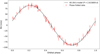 |
Fig. 12 Best-fit Keplerian model for XO-2N b (phase-folded), after removing the multidimensional GP. |
6.2 Limits on the masses of possible outer companions from Gaia and direct imaging
Further constraints on the mass of the detected planets and on the presence of additional companions can in principle be derived from high-precision absolute astrometry. However, the XO-2 star system was not observed by HIPPARCOS, ruling out the possibility of exploiting the sensitive Gaia-HIPPARCOS proper motion anomaly (Kervella et al. 2022) and at d ≃ 150 pc the constraints from Gaia alone are not very informative. The Gaia DR3 time span covers only ~20% of the orbit of XO-2S d. The Renormalized Unit Weight Error (RUWE) statistics (Lindegren et al. 2021) can be used to find indications of a statistically significant departure from a good single-star fit, typically when RUWE ≳ 1.4. For XO-2S, the Gaia archive reports RUWE = 0.88, providing no indication of the presence of orbital motion. Following the approach described in Blanco-Pozo et al. (2023) and Kunimoto et al. (2023), we estimated that at the separation of 5.4 au there is a probability >90% of obtaining RUWE > 0.88 for true companion masses ≳60 MJup, ruling out only inclination angles ≲4°.
Additional constraints at wider separation can be inferred by the proper motion differences. Considering the individual components, there are marginally significant differences between proper motion in right ascension from Gaia DR3 and the one from Tycho2 and PPMXL catalogs, while UCAC5 agrees within errors. However, we noticed that such differences are similar in magnitude and sign for both components, suggesting that they are mostly due to systematic errors in the pre-Gaia catalogs, as found by, for example, Lindegren et al. (2016) and Shi et al. (2019), rather than to the presence of additional bodies or to the orbital motion of the binary.
From the proper motion differences in Gaia DR3, we derive an instantaneous (at Gaia DR3 epoch) velocity difference of 171 + 15 m s−1 and 3± 15 m s−1 in right ascension and declination directions, respectively. The velocity difference along the line of sight is instead derived from the difference of the center of mass velocities from the orbital fits in Sect. 4.3–5.5. This amounts to 346+12 m s−1.8 Therefore, it results that the total velocity difference between the components is 386+24 m s−1, for a projected separation of 4685 au on the plane of the sky. The physical separation along the line of sight remains unknown, as the individual parallaxes agree to better than 1 σ, but a broad range of values is compatible with a bound orbit for XO-2N and XO-2S. We conclude that the observed differences between the components in RV and proper motion are fully consistent with those expected from orbital motion in a bound orbit, and the presence of additional massive companions is not required.
Finally, we note that both Gaia and dedicated imaging observations of XO-2N (Daemgen et al. 2009; Ngo et al. 2015) did not reveal additional sources close to the star, ruling out any stellar companion at projected separations from 150 to 1500 au, and with detection limits of about 0.28 M⊙ at 30 au. For XO-2S, there are no imaging observations on the target; relying on detection limits for close companions from Gaia (Brandeker & Cataldi 2019), companions more massive than 0.5, 0.25, 0.10 M⊙ are ruled out at projected separations of 180, 300, and 700 au, respectively.
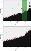 |
Fig. 13 Detection function maps of the RV time series of XO-2S (upper panel) and XO-2N (lower panel). The white part corresponds to the area in the period-minimum mass space where additional signals could be detected if present in the data, while the black region corresponds to the area where the detection probability is negligible. The red dotted line marks the 95% detection threshold. The cyan dots show the positions of the planets orbiting the two stars. The green shaded area in the upper panel denotes the stability region discussed in Sect. 4.5. The orange dashed line and shaded band in the lower panel mark the period and 1σ uncertainty of the activity cycle as modeled in Sect. 5.5. |
6.3 Revisiting the origin of the elemental abundances difference
Ramírez et al. (2015) and Biazzo et al. (2015) discussed about the significant difference of the XO-2N abundance relative to XO-2S and the trends with the condensation temperature (Tcond). They interpreted their results as the signature of the ingestion of material by XO-2N or depletion in XO-2S due to the locking of heavy elements by planetary companions. As described in the previous sections, we now have evidence for a new massive planet in the XO-2S system, while we ruled out a Keplerian origin for the long-term RV variations of XO-2N, excluding additional massive planets within several au. This leads to a large difference between the two stars in terms of total hosted planetary mass. In particular, we have a total minimum planetary mass of 5.35 MJ for XO-2S and a true mass of 0.6 MJ for XO-2N, so the ratio is approximately a factor of ten. In addition, since in the last years, some steps have been made in the field of abundance differences in binary components, here in the following we update possible implications related to the difference observed in the XO-2 system.
In order to better quantify and possibly validate the scenario of planetary material ingestion, we used the code terra9 (Yana Galarza et al. 2016), which first computes the convective mass of a solar-type star, and then estimates the mass of the rocky material missing in the convective zone. The convective mass is calculated considering the mass and the metallicity of the star and adopting the Yale isochrones of stellar evolution by Yi et al. (2001). Once the convective mass is obtained, the code computes the amount of rocky material necessary to reproduce the observed abundance pattern by adding meteoritic (Wasson & Kallemeyn 1988) and terrestrial (Allègre et al. 2001) abundance patterns into the convective zone of the star (see Yana Galarza et al. 2016; Galarza et al. 2021 for more details). Considering the stellar mass and iron abundance found by Damasso et al. (2015), the differential abundance pattern found by Biazzo et al. (2015) can be explained by a rocky planet engulfment of ~8.5 M⊕, which is a mixture of ~2 M⊕ of chondrite-like composition and ~6.5 M⊕ of Earth-like composition. As can be seen in Fig. 14, the predicted (red filled circles) differential abundances seem to be smaller than those observed (open blue squares) for the elements with condensation temperature higher than ~1500 K. Similar behavior happens also applying the same procedure to the results of Ramírez et al. (2015; see lower panel of Fig. 14), thus implying that possibly other scenarios, such as the locking of heavy elements around XO-2S, besides planet accretion onto XO-2N, could be the reason of the observed trend. However, to our knowledge, there are still no theoretical models predicting the amount of locking of heavy elements due to the presence of planetary companions. The scenario is also complicated by the presence of a multiple system around the S component with no transiting planets which prevents the determination of the planet density, whose value could be related to the content of heavy elements (see, e.g., Biazzo et al. 2022, and references therein). At the same time, if the planet engulfment scenario is correct, the rotation of XO-2N should be faster than XO-2S (see Oetjens et al. 2020). However, there is no significant difference in the homogeneously derived projected rotational velocity of the components, resulting in consistent v sin i within the errors (see Biazzo et al. 2022). This finding does not invalidate the hypothesis of planet ingestion because the planetary engulfment could have happened when the star was young, implying that the increase in angular momentum due to the planet has already been lost. Recent models indeed claim that engulfment events last no longer than ~2 Gyr and that the detection of possible engulfment is rare to be detected in systems that are several Gyr old (see Behmard et al. 2023).
Interestingly, the absolute differences in [Fe/H] (~0.055 dex), the absolute value of the slope of the Tcond trend (~4.7× 10⁻⁵ dex K−1 ), and the binary separation (4600 au) seem to be in line with the recent trends proposed by Liu et al. (2021, see their Figs. 15 and 16). The authors claim that the possible dependence of the [Fe/H] difference and the Tcond slope on the binary separation could indicate that the dynamical history of binaries has a potential impact on the process of planet formation. Although still speculative, it is possible that the architecture of planetary systems might be affected in binaries to some level, since the dynamical interaction and the binary separation are relevant.
Another possible interpretation of the observed trends between the differential elemental abundances and the condensation temperatures could be offered by the framework of the gas-dust segregation scenario (Gaidos 2015). Based on this idea, Booth & Owen (2020) developed an evolutionary model to test if, during the giant planet formation, the gas-dust segregation process operating across a protoplanetary disk could produce chemical imprints. The authors demonstrated that a distant forming giant planet can open gaps in the disk, creating a pressure trap and allowing the gas to be accreted onto the protostar. In contrast, if the planet forms early enough when the disk is still massive, the planet can trap a substantial mass of dust exterior to its orbit preventing the dust from accreting onto the star in contrast to the gas. This could result in refractory element deficiency of 5-15%, with the larger values occurring for conditions favoring giant planet formation around more massive and longer-lived disks. Taking into account the results by the authors and the mean elemental abundance difference between the N and the S components of +0.067 ± 0.032 dex (Biazzo et al. 2015), the lack of refractory elements of the S component relative to the N companion maybe was produced through a gas-dust segregation mechanism at the early formation of its distant giant planet XO-2Sd (a ~ 5.5 au, m sin i ~ 3.7 MJ; see Table 3). However, the statistically significant trend observed with the condensation temperature for the individual elements cannot still be explained with this model.
On the observational side, we mention that Ramírez et al. (2015) and Biazzo et al. (2015) also found hints of break-in Tcond between volatile and refractory elements at -800 K possibly related to the distance where the planets form along the protoplanetary disk. Theoretical simulations by Bitsch et al. (2018) showed that a planet formed inside the H2O/CO ice line can produce a much larger difference in its host stars’ surface abundance ratios ([Fe/O] and [Fe/C]) than for planets formed out of the H2O/CO ice line. This is because at the disk location interior to the snow lines, the accreted core is volatile-depleted and the host stars would reveal a high abundance of volatile elements compared to the refractory ones. Following this hypothesis, the higher values of these elemental ratios found for XO-2N ([Fe/O] = 0.050, [Fe/C] = −0.040) compared to XO-2S ([Fe/O] = −0.045, [Fe/C] = −0.045) could be indicative of the possible different location of the forming planets along the protoplanetary disks around the binary components.
The evaluation of these scenarios remains rather speculative at this stage. Further inputs might come on one side from additional modeling of the impact of planet formation processes on star elemental abundances, on the other side from a better understanding of the most probable formation sites and evolutionary histories of the planets in the system, through, for instance, population synthesis of the two systems (Mordasini 2018) and more complete characterization of the transiting planet XO-2N b. Indeed, the only species significantly detected so far are potassium (Sing et al. 2011) and sodium (Sing et al. 2012). Pearson et al. (2019) spectrally resolved sodium and were able to set a slightly substellar lower limit to the abundance of this element by resolving the wings of the doublet, but unfortunately – because alkali elements are susceptible to ionization, and undetected clouds could bias the inferred abundances – it is not possible to draw firm conclusions on the overall atmospheric enrichment of XO-2N b based on this measurement.
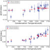 |
Fig. 14 Comparison of the abundances of XO-2N relative to XO-2S (open blue squares) as a function of the dust condensation temperature, and the predicted abundances (red filled circles) estimated from a planetary engulfment scenario. Squares in the upper and lower panels represent the results by Biazzo et al. (2015) and Ramírez et al. (2015), respectively. |
7 Conclusion
In this paper, we analyzed the XO-2 system that had already been shown to be a unique benchmark for studying the stochasticity of planet formation. Indeed, it is a binary system with nearly identical components, apart from a small difference in chemical abundances, both with a planetary system but with markedly different characteristics. Greatly extending the time coverage of our HARPS-N RV monitoring, we were able to further confirm the known planets and show evidence for an additional massive long-period giant planet around XO-2S in a Jupiter-like orbit. In addition, we found no evidence for the transits of its two inner planets, ruling out inclinations close to an edge-on configuration. Furthermore, we showed that, even for highly inclined orbits, the system remains stable and there are fairly broad stability regions where low-mass planets could be present but undetectable at present.
On the other hand, for XO-2N we showed that the additional long-term RV signal is likely due to a Solar-like activity cycle rather than a second planet. Therefore, the known planet XO-2N b appears to be a single transiting hot Jupiter, although detection limits for additional companions are poorer than those of XO-2S because of the lower amount of data and the higher effect of stellar activity. Astrometry and direct imaging datasets have limited sensitivity but they do not support the presence of additional massive companions at large separations.
With these results, the known planetary system of XO-2N has a total mass of 0.59 MJ, while that of XO-2S has a minimum mass of 5.35 MJ. This means that, even though the two stars are almost physically identical, the more metallic one has one order of magnitude less planetary mass than the other. This might indicate that mechanisms related to the segregation of dust grains in planetary cores and atmospheres could be at work, although more detailed work, especially on the modeling side, is needed to reach firm conclusions. In any case, the XO-2 system remains and becomes, even more after the new results of this paper, a unique laboratory to understand the diversity of the outcomes of the planet formation process.
Acknowledgements
We acknowledge the financial support from the agreement ASI-INAF n.2018-16-HH.0. This work has made use of data from the European Space Agency (ESA) mission Gaia (https://www.cosmos.esa.int/gaia), processed by the Gaia Data Processing and Analysis Consortium (DPAC, https://www.cosmos.esa.int/web/gaia/dpac/consortium). Funding for the DPAC has been provided by national institutions, in particular, the institutions participating in the Gaia Multilateral Agreement. We acknowledge the use of public TESS data from pipelines at the TESS Science Office and at the TESS Science Processing Operations Center. Resources supporting this work were provided by the NASA High-End Computing (HEC) Program through the NASA Advanced Supercomputing (NAS) Division at Ames Research Center for the production of the SPOC data products.
References
- Allègre, C., Manhès, G., & Lewin, É. 2001, Earth Planet. Sci. Lett., 185, 49 [CrossRef] [Google Scholar]
- Behmard, A., Dai, F., Brewer, J. M., Berger, T. A., & Howard, A. W. 2023, MNRAS, 521, 2969 [NASA ADS] [CrossRef] [Google Scholar]
- Benatti, S., Desidera, S., Damasso, M., et al. 2017, A&A, 599, A90 [NASA ADS] [CrossRef] [EDP Sciences] [Google Scholar]
- Biazzo, K., Gratton, R., Desidera, S., et al. 2015, A&A, 583, A135 [NASA ADS] [CrossRef] [EDP Sciences] [Google Scholar]
- Biazzo, K., D’Orazi, V., Desidera, S., et al. 2022, A&A, 664, A161 [NASA ADS] [CrossRef] [EDP Sciences] [Google Scholar]
- Bitsch, B., Forsberg, R., Liu, F., & Johansen, A. 2018, MNRAS, 479, 3690 [NASA ADS] [CrossRef] [Google Scholar]
- Blanco-Pozo, J., Perger, M., Damasso, M., et al. 2023, A&A, 671, A50 [NASA ADS] [CrossRef] [EDP Sciences] [Google Scholar]
- Booth, R. A., & Owen, J. E. 2020, MNRAS, 493, 5079 [NASA ADS] [CrossRef] [Google Scholar]
- Brandeker, A., & Cataldi, G. 2019, A&A, 621, A86 [NASA ADS] [CrossRef] [EDP Sciences] [Google Scholar]
- Burke, C. J., McCullough, P. R., Valenti, J. A., et al. 2007, ApJ, 671, 2115 [NASA ADS] [CrossRef] [Google Scholar]
- Butler, R. P., Vogt, S. S., Laughlin, G., et al. 2017, AJ, 153, 208 [Google Scholar]
- Cincotta, P. M., & Simó, C. 2000, A&AS, 147, 205 [NASA ADS] [CrossRef] [EDP Sciences] [Google Scholar]
- Cosentino, R., Lovis, C., Pepe, F., et al. 2012, SPIE Conf. Ser., 8446, 84461V [Google Scholar]
- Covino, E., Esposito, M., Barbieri, M., et al. 2013, A&A, 554, A28 [NASA ADS] [CrossRef] [EDP Sciences] [Google Scholar]
- Daemgen, S., Hormuth, F., Brandner, W., et al. 2009, A&A, 498, 567 [NASA ADS] [CrossRef] [EDP Sciences] [Google Scholar]
- Damasso, M., Biazzo, K., Bonomo, A. S., et al. 2015, A&A, 575, A111 [NASA ADS] [CrossRef] [EDP Sciences] [Google Scholar]
- Desidera, S., Bonomo, A. S., Claudi, R. U., et al. 2014, A&A, 567, L6 [NASA ADS] [CrossRef] [EDP Sciences] [Google Scholar]
- Eggenberger, A., & Udry, S. 2010, EAS Pub. Ser., 41, 27 [NASA ADS] [CrossRef] [EDP Sciences] [Google Scholar]
- Foreman-Mackey, D., Hogg, D. W., Lang, D., & Goodman, J. 2013, PASP, 125, 306 [Google Scholar]
- Gaidos, E. 2015, ApJ, 804, 40 [NASA ADS] [CrossRef] [Google Scholar]
- Galarza, J. Y., López-Valdivia, R., Meléndez, J., & Lorenzo-Oliveira, D. 2021, ApJ, 922, 129 [NASA ADS] [CrossRef] [Google Scholar]
- Gelman, A., & Rubin, D. B. 1992, Statist. Sci., 7, 457 [NASA ADS] [Google Scholar]
- Gomes da Silva, J., Figueira, P., Santos, N., & Faria, J. 2018, J. Open Source Softw., 3, 667 [Google Scholar]
- Gomes da Silva, J., Santos, N. C., Adibekyan, V., et al. 2021, A&A, 646, A77 [NASA ADS] [CrossRef] [EDP Sciences] [Google Scholar]
- Gozdziewski, K., Bois, E., Maciejewski, A. J., & Kiseleva-Eggleton, L. 2001, A&A, 378, 569 [NASA ADS] [CrossRef] [EDP Sciences] [Google Scholar]
- Grunblatt, S. K., Howard, A. W., & Haywood, R. D. 2015, ApJ, 808, 127 [NASA ADS] [CrossRef] [Google Scholar]
- Hippke, M., & Heller, R. 2019, A&A, 623, A39 [NASA ADS] [CrossRef] [EDP Sciences] [Google Scholar]
- Husser, T.-O., Wende-von Berg, S., Dreizler, S., et al. 2013, A&A, 553, A6 [NASA ADS] [CrossRef] [EDP Sciences] [Google Scholar]
- Ivshina, E. S., & Winn, J. N. 2022, ApJS, 259, 62 [CrossRef] [Google Scholar]
- Jenkins, J. M., Twicken, J. D., McCauliff, S., et al. 2016, SPIE, 9913, 99133E [NASA ADS] [Google Scholar]
- Jones, H. R. A., Butler, R. P., Tinney, C. G., et al. 2006, MNRAS, 369, 249 [CrossRef] [Google Scholar]
- Kane, S. R. 2007, MNRAS, 380, 1488 [NASA ADS] [CrossRef] [Google Scholar]
- Kass, R. E., & Raftery, A. E. 1995, J. Am. Statist. Assoc., 90, 773 [CrossRef] [Google Scholar]
- Kervella, P., Arenou, F., & Thévenin, F. 2022, A&A, 657, A7 [NASA ADS] [CrossRef] [EDP Sciences] [Google Scholar]
- Kreidberg, L. 2015, PASP, 127, 1161 [Google Scholar]
- Kunimoto M. Vanderburg, A., Huang, C. X. et al. 2023 AJ 166 7 [NASA ADS] [CrossRef] [Google Scholar]
- Lanza, A. F., Rodonò, M., & Pagano, I. 2004, A&A, 425, 707 [NASA ADS] [CrossRef] [EDP Sciences] [Google Scholar]
- Lanza, A. F., Molaro, P., Monaco, L., & Haywood, R. D. 2016, A&A, 587, A103 [NASA ADS] [CrossRef] [EDP Sciences] [Google Scholar]
- Lightkurve Collaboration, (Cardoso, J. V. d. M., et al.) 2018, Astrophysics Source Code Library [record ascl:1812.013] [Google Scholar]
- Lindegren, L., Lammers, U., Bastian, U., et al. 2016, A&A, 595, A4 [NASA ADS] [CrossRef] [EDP Sciences] [Google Scholar]
- Lindegren, L., Klioner, S. A., Hernández, J., et al. 2021, A&A, 649, A2 [EDP Sciences] [Google Scholar]
- Lissauer, J. J., Marcy, G. W., Bryson, S. T., et al. 2014, ApJ, 784, 44 [NASA ADS] [CrossRef] [Google Scholar]
- Liu, F., Bitsch, B., Asplund, M., et al. 2021, MNRAS, 508, 1227 [NASA ADS] [CrossRef] [Google Scholar]
- Lovis, C., Dumusque, X., Santos, N. C., et al. 2011, arXiv e-prints [arXiv:1107.5325] [Google Scholar]
- Malavolta, L., Nascimbeni, V., Piotto, G., et al. 2016, A&A, 588, A118 [NASA ADS] [CrossRef] [EDP Sciences] [Google Scholar]
- Malavolta, L., Mayo, A. W., Louden, T., et al. 2018, AJ, 155, 107 [NASA ADS] [CrossRef] [Google Scholar]
- Mamajek, E. E., & Hillenbrand, L. A. 2008, ApJ, 687, 1264 [Google Scholar]
- Mantovan, G., Montalto, M., Piotto, G., et al. 2022, MNRAS, 516, 4432 [NASA ADS] [CrossRef] [Google Scholar]
- McLaughlin, D. B. 1924, ApJ, 60, 22 [Google Scholar]
- Mordasini, C. 2018, in Handbook of Exoplanets, eds. H. J. Deeg, & J. A. Belmonte (Berlin: Springer), 143 [Google Scholar]
- Narita, N., Hirano, T., Sato, B., et al. 2011, PASJ, 63, L67 [NASA ADS] [Google Scholar]
- Neveu-VanMalle, M., Queloz, D., Anderson, D. R., et al. 2014, A&A, 572, A49 [NASA ADS] [CrossRef] [EDP Sciences] [Google Scholar]
- Ngo, H., Knutson, H. A., Hinkley, S., et al. 2015, ApJ, 800, 138 [Google Scholar]
- Noyes, R. W., Hartmann, L. W., Baliunas, S. L., Duncan, D. K., & Vaughan, A. H. 1984, ApJ, 279, 763 [Google Scholar]
- Oetjens, A., Carone, L., Bergemann, M., & Serenelli, A. 2020, A&A, 643, A34 [NASA ADS] [CrossRef] [EDP Sciences] [Google Scholar]
- Parviainen, H., & Aigrain, S. 2015, MNRAS, 453, 3821 [Google Scholar]
- Pearson, K. A., Griffith, C. A., Zellem, R. T., Koskinen, T. T., & Roudier, G. M. 2019, AJ, 157, 21 [NASA ADS] [CrossRef] [Google Scholar]
- Pinamonti, M., Sozzetti, A., Maldonado, J., et al. 2022, A&A, 664, A65 [NASA ADS] [CrossRef] [EDP Sciences] [Google Scholar]
- Raghavan, D., McAlister, H. A., Henry, T. J., et al. 2010, ApJS, 190, 1 [Google Scholar]
- Rajpaul, V., Aigrain, S., Osborne, M. A., Reece, S., & Roberts, S. 2015, MNRAS, 452, 2269 [Google Scholar]
- Ramírez, I., Khanal, S., Aleo, P., et al. 2015, ApJ, 808, 13 [Google Scholar]
- Ricker, G. R., Winn, J. N., Vanderspek, R., et al. 2015, J. Astron. Telesc. Instrum. Syst., 1, 014003 [Google Scholar]
- Rossiter, R. A. 1924, ApJ, 60, 15 [Google Scholar]
- Schwarz, G. 1978, Ann. Stat., 6, 461 [Google Scholar]
- Shi, Y. Y., Zhu, Z., Liu, N., et al. 2019, AJ, 157, 222 [NASA ADS] [CrossRef] [Google Scholar]
- Sing, D. K., Désert, J. M., Fortney, J. J., et al. 2011, A&A, 527, A73 [NASA ADS] [CrossRef] [EDP Sciences] [Google Scholar]
- Sing, D. K., Huitson, C. M., Lopez-Morales, M., et al. 2012, MNRAS, 426, 1663 [CrossRef] [Google Scholar]
- Storn, R., & Price, K. 1997, J. Glob. Optim., 11, 341 [Google Scholar]
- Teske, J. K., Ghezzi, L., Cunha, K., et al. 2015, ApJ, 801, L10 [NASA ADS] [CrossRef] [Google Scholar]
- Udry, S., Dumusque, X., Lovis, C., et al. 2019, A&A, 622, A37 [NASA ADS] [CrossRef] [EDP Sciences] [Google Scholar]
- Wasson, J. T., & Kallemeyn, G. W. 1988, Philos. Trans. R. Soc. London Ser. A, 325, 535 [CrossRef] [Google Scholar]
- Yana Galarza, J., Meléndez, J., Ramírez, I., et al. 2016, A&A, 589, A17 [NASA ADS] [CrossRef] [EDP Sciences] [Google Scholar]
- Yi, S., Demarque, P., Kim, Y.-C., et al. 2001, ApJS, 136, 417 [Google Scholar]
- Zechmeister, M., & Kürster, M. 2009, A&A, 496, 577 [CrossRef] [EDP Sciences] [Google Scholar]
- Zellem, R. T., Griffith, C. A., Pearson, K. A., et al. 2015, ApJ, 810, 11 [NASA ADS] [CrossRef] [Google Scholar]
This definition arises from the fact that in most cases, the GP regression analysis is performed for stars for which the dominant stellar contribution to RV variability is due to rotational modulation. Nevertheless, the same formalism can also be used for activity cycles.
The uncertainty here includes the measurement uncertainty only. In general, when comparing the absolute RV of two stars, differences in convective blueshift and gravitational redshift are significant as well as color-dependent RV zero point errors, due to, for example, cross-correlation mask mismatch. However, these sources of errors are expected to be very small in the comparison of XO-2N and XO-2S, considering the very similar stellar properties and the common instrument setup.
All Tables
All Figures
|
Fig. 1 TESS light curves of XO-2S after removing outliers above 4 σ, normalizing, correcting for dilution, and removing the transits of XO-2N b. The red bars indicate the predicted transits for planet b from RV results, as explained in Sect. 4.4. |
| In the text | |
|
Fig. 2 GLS of the RV residuals of XO-2S after removing the signal corresponding to planet c. The peak at 18.2 d corresponds to planet b. |
| In the text | |
|
Fig. 3 Best-fit model (Model 2) of XO-2S. |
| In the text | |
|
Fig. 4 Best-fit Keplerian model for XO-2S b (phase-folded), after removing the RV signal of the other two planets. |
| In the text | |
|
Fig. 5 Best-fit Keplerian model for XO-2S c (phase-folded), after removing the RV signal of the other two planets. |
| In the text | |
|
Fig. 6 Best-fit Keplerian model for XO-2S d, after removing the RV signal of the other two planets. |
| In the text | |
|
Fig. 7 Corner plot of the orbital parameters of the new candidate XO-2S d obtained from our analysis. |
| In the text | |
|
Fig. 8 Stability results using the chaos indicator MEGNO (color bar on the right) for XO-2S, using the nominal values for the masses of the three planets. |
| In the text | |
|
Fig. 9 Stability results using the chaos indicator MEGNO (color bar on the right) for XO-2S, increasing the masses of the three planets by a factor of 3 with respect to the m sin i. |
| In the text | |
|
Fig. 10 Periodograms of XO-2N. Left panel: GLS of RV residuals of XO-2N obtained from a 1-planet model without activity. Central panel: GLS of the BIS data of XO-2N. Right panel: GLS of the SMW activity index of XO-2N. |
| In the text | |
|
Fig. 11 Correlations between RV residuals and activity indicators of XO-2N. Left panel: correlation between SMW and RV residuals. Right panel: same correlation but between the BIS indicator and RV residuals. |
| In the text | |
|
Fig. 12 Best-fit Keplerian model for XO-2N b (phase-folded), after removing the multidimensional GP. |
| In the text | |
|
Fig. 13 Detection function maps of the RV time series of XO-2S (upper panel) and XO-2N (lower panel). The white part corresponds to the area in the period-minimum mass space where additional signals could be detected if present in the data, while the black region corresponds to the area where the detection probability is negligible. The red dotted line marks the 95% detection threshold. The cyan dots show the positions of the planets orbiting the two stars. The green shaded area in the upper panel denotes the stability region discussed in Sect. 4.5. The orange dashed line and shaded band in the lower panel mark the period and 1σ uncertainty of the activity cycle as modeled in Sect. 5.5. |
| In the text | |
|
Fig. 14 Comparison of the abundances of XO-2N relative to XO-2S (open blue squares) as a function of the dust condensation temperature, and the predicted abundances (red filled circles) estimated from a planetary engulfment scenario. Squares in the upper and lower panels represent the results by Biazzo et al. (2015) and Ramírez et al. (2015), respectively. |
| In the text | |
Current usage metrics show cumulative count of Article Views (full-text article views including HTML views, PDF and ePub downloads, according to the available data) and Abstracts Views on Vision4Press platform.
Data correspond to usage on the plateform after 2015. The current usage metrics is available 48-96 hours after online publication and is updated daily on week days.
Initial download of the metrics may take a while.