© The Authors 2024

1. Introduction

In a thermally isolated system, that is, when the variation of gas internal energy results only from mechanical work without heat exchange, the gas adiabatic index γ describes the relation between pressure P and density ρ, such that P ∝ ρ^γ. However, in astrophysical systems, cooling and heating mechanisms often come into play and act on a timescale that is sufficiently small compared to the dynamical timescale. The thermal behavior of the gas therefore deviates from adiabaticity. For convenience, an effective polytropic equation of state (EOS) is very often employed to avoid explicitly solving the energy equation in many contexts. An EOS following

$$\begin{array}{c}\hfill P\propto {\rho }^{\mathrm{\Gamma }},\end{array}$$(1)

where Γ is the polytropic index, is used to replace the energy conservation equation in a hydrodynamic system. This practice is widely accepted, given numerous supporting evidence, either observational (Myers 1978) or theoretical (Tarafdar et al. 1985; Boland & de Jong 1984; Larson 1973b).

The molecular interstellar medium (ISM) is known to be efficiently cooled due to the numerous molecular and atomic lines. The ISM cools from ∼1000 K at 1 cm⁻³ to ∼10 K at 10⁴ cm⁻³, which can be described with a polytropic index Γ ∼ 0.73 (Larson 1985). In the density range between 10⁴ and 10¹⁰ cm⁻³, the temperature is maintained at roughly 10 K. At higher densities, the dust component, which takes up only one percent of the mass fraction, starts to contribute significantly to the opacity, and the radiative heat loss becomes very inefficient. Therefore, many studies, without loss of generality, assume an isothermal behavior for the star-forming ISM, which only becomes adiabatic at high densities, corresponding to the first hydrostatic core formation.

The polytropic index is important for understanding the gas dynamics because it determines whether the energy balance allows gravitational collapse to occur. For collapse solution to exist, the critical value Γ_crit = 4/3 for spherical geometry, and is equal to unity for cylindrical geometry. Given a polytropic index larger than the critical value, gravitational contraction leads to increased gas internal energy and results in a thermally supported structure.

In the diffuse ISM, the heating mostly comes from the cosmic rays or background UV radiation, which can be regarded as almost constant. The volumetric heating thus scales linearly with the density. On the other hand, cooling usually results from the deexcitation of the collisionally excited molecules, and therefore scales quadratically with the density and has a steep nonlinear dependance on the temperature. When the dynamical timescale of the system is significantly longer than the heating and cooling timescales, the gas temperature is simply determined through the balance between the two latter mechanisms. The present work considers the regime where the cooling timescale is greater than, or at least comparable to, the dynamic or thermal sound crossing time. Therefore, the cooling modifies the thermal behavior during the collapse, instead of reaching instantaneous equilibrium with other heating mechanisms.

The purpose of the present study is to derive the effective polytropic index, Γ, from a parametric cooling function that is a power-law product of density and temperature, Λ ∝ ρ^mTⁿ. We solve the full hydrodynamic equations, adding a cooling term to the energy equation, and look for self-similar solutions. The solutions are then used to understand the apparent polytropic behavior of the collapsing gas. We successfully demonstrate that a gas element evolves along a polytrope with the material polytropic index, Γ_M = 1 + (3/2 − m)/(n − 1), in the flat center of a cloud under homologous collapse, and with Γ_M = 1 + (2 − m)/(n − 1) during the accretion phase onto the central mass singularity. However, when profiling the cloud as an ensemble, the thus derived apparent polytropic index, Γ_A, has different values in different cloud regions. We clarify in this work that such a polytropic index measured with the temperature-density relation of instantaneous profiles does not reflect directly the thermodynamic properties of the cloud, and that their usage should not be confused.

2. Formalism

2.1. The physical system

The compressible Navier-Stokes equations with cooling writes

$$\begin{array}{cc}& \frac{\partial \rho }{\partial t}+\mathbf{\nabla }·(\rho \mathit{u})=0,\hfill \end{array}$$(2)

$$\begin{array}{cc}& \frac{\partial \rho \mathit{u}}{\partial t}+\mathrm{\nabla }·(\rho \mathit{u}\mathit{u})=-\mathbf{\nabla }P-\rho \mathbf{\nabla }\varphi ,\hfill \end{array}$$(3)

$$\begin{array}{cc}& \mathrm{\Delta }\varphi =4\pi G\rho ,\hfill \end{array}$$(4)

$$\begin{array}{cc}& \frac{\partial \rho (ϵ+\frac{u^2}{2})}{\partial t}+\mathbf{\nabla }·\left[\rho (ϵ+\frac{u^2}{2})\mathit{u}\right]=-\mathbf{\nabla }·(P\mathit{u})-\rho \mathit{u}·\mathbf{\nabla }\varphi -\mathrm{\Lambda },\hfill \end{array}$$(5)

where t is time, u is the velocity vector, ϕ is the gravitational potential, G is the gravitational constant, ϵ is the specific internal energy, and Λ the volumetric cooling rate. The heat exchange includes heating and cooling, while here we only discuss the regime where cooling is more important than heating and there is a net energy loss. The gas follows the ideal gas law,

$$\begin{array}{c}\hfill \frac{k_{\mathrm{B}}}{\mu m_{\mathrm{p}}}T=\frac{P}{\rho }=(\gamma -1)ϵ,\end{array}$$(6)

where k_B is the Boltzmann constant, μ is the mean particle (molecular) weight, m_p is the proton mass, and T is the temperature. By parameterizing the cooling function as

$$\begin{array}{c}\hfill \mathrm{\Lambda }={\mathrm{\Lambda }}_0{\rho }^m{T}^n,{\mathrm{\Lambda }}_0\in {\mathcal{R}}^{+},\end{array}$$(7)

the equation set can be rewritten for a one-dimensional system in spherical symmetry:

$$\begin{array}{cc}& \frac{\partial \rho }{\partial t}+\frac{1}{r^2}\frac{\partial r^2\rho u}{\partial r}=0,\hfill \end{array}$$(8)

$$\begin{array}{cc}& \frac{\partial u}{\partial t}+u\frac{\partial u}{\partial r}=-\frac{1}{\rho }\frac{\partial P}{\partial r}-\frac{\partial \varphi }{\partial r},\hfill \end{array}$$(9)

$$\begin{array}{cc}& \frac{1}{r^2}\frac{\partial }{\partial r}\left(r^2\frac{\partial \varphi }{\partial r}\right)=4\pi G\rho ,\hfill \end{array}$$(10)

$$\begin{array}{cc}& \rho (\frac{\partial ϵ}{\partial t}+u\frac{\partial ϵ}{\partial r})=-\frac{P}{r^2}\frac{\partial r^{2}u}{\partial r}-{\mathrm{\Lambda }}_0{\rho }^m{T}^n.\hfill \end{array}$$(11)

2.2. Cooling models in the literature

The radiative cooling functions were calculated from first principles (e.g., Hollenbach & McKee 1979; Neufeld & Kaufman 1993; Neufeld et al. 1995; Omukai 2001), and were applied to and tested in many studies¹. In general, the cooling due to collision-induced radiations scales quadratically with the density (m = 2) and linearly with the abundance of the cooling agent in question. On the other hand, with increased optical depth reaching local thermal equilibrium (LTE), cooling scales linearly with the density of the cooling agent (total density multiplied by the abundance; m = 1). However, we can still assume that the photons can escape efficiently once they exit the local region where they are emitted due to the large velocity gradients inside the cloud.

There have been many theoretical models of the cooling gas temperature, while a full collapse solution has not been proposed due to the complexity of the problem. For example, Goldsmith (2001) considered a static one-zone model and studied the effect of depletion on molecular cooling. They concluded that m ≈ 2 and 1.4 < n < 3.8 for the major coolants at low densities (between 10² and 10⁷). Hunter (1969), Disney et al. (1969), and Larson (1973a) considered simplified, stationary models of balancing heating by cosmic rays and compression against cooling by atomic lines and dust emission, and assuming uniform density for the estimated optical depth. This simplified calculation already allowed the characteristic behavior of the cloud to be inferred. They all reached very similar conclusions, that is, isothermality during collapse, while they did not specify whether the center is in free fall or not. In the density range between 10⁵ and 10¹¹ cm⁻³, the cooling process is strongly coupled to dust grains and is very sensitive to temperature (∝T⁷; Larson 1973b). As we demonstrate in Sect. 3.1, the apparent EOS is indeed close to isothermality when the temperature dependence is steep.

2.3. Self-similar equations

Following the transformation of Murakami et al. (2004),

$$\begin{array}{c}\hfill r=\lambda \widehat{r},t={\lambda }^a\widehat{t},u={\lambda }^b\widehat{u},T={\lambda }^c\widehat{T},\rho ={\lambda }^d\widehat{\rho },\varphi ={\lambda }^e\widehat{\varphi },\end{array}$$(12)

we look for a self-similar system. For self-similar solution to exist, the system must satisfy

$$\begin{array}{c}\hfill 1-a=b=\frac{c}{2}=1+\frac{d}{2}=\frac{e}{2}=\frac{3-2m}{5-2m-2n}.\end{array}$$(13)

We chose the similarity ansatz:

$$\begin{array}{cc}& r={A|t|}^{1/a}\xi ,\hfill \end{array}$$(14)

$$\begin{array}{cc}& u=\frac{A}{a}{|t|}^{b/a}v(\xi ),\hfill \end{array}$$(15)

$$\begin{array}{cc}& T={\left(\frac{A}{a}\right)}^2\frac{\mu m_{\mathrm{p}}}{k_{\mathrm{B}}}{|t|}^{c/a}\tau (\xi ),\hfill \end{array}$$(16)

$$\begin{array}{cc}& \rho ={B|t|}^{-2}g(\xi ),\hfill \end{array}$$(17)

$$\begin{array}{cc}& \frac{\partial \varphi }{\partial r}=\frac{4\pi GAB}{{\xi }^2}{|t|}^{(e-1)/a}\mathrm{\Omega }(\xi ),\hfill \end{array}$$(18)

$$\begin{array}{cc}& M=M_0+4\pi {\displaystyle \underset{0}{\overset{r}{\int }}}{r}^2\rho \mathrm{d}r=4\pi A^{3}B{|t|}^{(3-2a)/a}\mathrm{\Omega }(\xi ),\hfill \end{array}$$(19)

$$\begin{array}{cc}& \mathrm{\Omega }(\xi )\equiv {\mathrm{\Omega }}_0+{\displaystyle \underset{0}{\overset{\xi }{\int }}}{\xi }^{2}g(\xi )\mathrm{d}\xi .\hfill \end{array}$$(20)

Here A, B ∈ ℛ⁺ are free parameters, the physical meanings of which are explained later. The time zero t = 0 corresponds to the epoch of formation of the central singular mass M₀, or Ω₀ in dimensionless form. Solutions should exist for t < 0 and for t > 0, corresponding to the collapse phase and accretion phase, respectively. The two phases are connected at ξ = ∞.

The dimensionless ODE set has the form

$$\begin{array}{cc}& (v\mp \xi )g^{\prime }+(\pm d+v^{\prime }+\frac{2v}{\xi })g=0,\hfill \end{array}$$(21)

$$\begin{array}{cc}& \pm bv+(\mp \xi +v)v^{\prime }+\frac{g^{\prime }\tau +g{\tau }^{\prime }}{g}+\frac{K_1\mathrm{\Omega }}{{\xi }^2}=0,\hfill \end{array}$$(22)

$$\begin{array}{cc}& \frac{\pm c\tau \mp \xi {\tau }^{\prime }+v{\tau }^{\prime }}{\gamma -1}+\tau v^{\prime }+\frac{2\tau v}{\xi }+K_2{g}^{m-1}{\tau }^n=0,\hfill \end{array}$$(23)

where the lower and upper signs correspond to t < 0 and t > 0, respectively. From the mass conservation law ∂M/∂t = −4πr²ρu, one derives

$$\begin{array}{c}\hfill \mathrm{\Omega }=\frac{{\xi }^{2}g(\xi \mp v)}{3-2a}.\end{array}$$(24)

The constants

$$\begin{array}{cc}& K_1=4\pi a^{2}GB,\hfill \end{array}$$(25)

$$\begin{array}{cc}& K_2={\mathrm{\Lambda }}_{0}a{B}^{m-1}{\left(\frac{A}{a}\right)}^{2(n-1)}{\left(\frac{\mu m_{\mathrm{p}}}{k_{\mathrm{B}}}\right)}^n.\hfill \end{array}$$(26)

Alternatively,

$$\begin{array}{cc}& A=|a|{\left(\frac{k_{\mathrm{B}}}{\mu m_{\mathrm{p}}}\right)}^{\frac{n}{2(n-1)}}{\left(\frac{K_2{B}^{1-m}}{{\mathrm{\Lambda }}_{0}a}\right)}^{\frac{1}{2(n-1)}},\hfill \end{array}$$(27)

$$\begin{array}{cc}& B=\frac{K_1}{4\pi a^{2}G}.\hfill \end{array}$$(28)

When the absolute value of the cooling function is lower, the physical extent of the dimensional system is correspondingly larger. On the other hand, the central density of the system is fixed by the values of m and n. We note that a physical solution exists only for K₁, Ω ∈ ℛ⁺, which signify density and mass positivity. Net cooling (Λ₀ > 0) requires K₂ to be of the same sign as a.

3. Results

We adopt the nomenclature by Whitworth & Summers (1985), and identify three regimes: early interior path (t < 0 and small ξ), exterior path (large ξ), and late path (t > 0 and small ξ). There is no analytical solution for this nonlinear system (except for one trivial solution at t < 0; see Appendix A), while we can derive asymptotic solutions in limiting conditions and perform numerical integration to obtain the full solutions.

3.1. Asymptotic behaviors of the self-similar system

The asymptotic solutions allow us to analytically evaluate the polytropic indices in the characteristic regimes of the collapsing cloud, and also serve as boundary conditions for numerical integration. The asymptotes are presented directly here and we refer to Appendix B for detailed derivations. We show the thus-derived apparent (instantaneous) polytropic indices

$$\begin{array}{c}\hfill {\mathrm{\Gamma }}_A-1={\frac{\mathrm{d}logT}{\mathrm{d}log\rho }|}_t=\frac{\partial logT/\partial r}{\partial log\rho /\partial r}\end{array}$$(29)

as functions of m and n for the three regimes in Fig. 1.

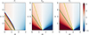Fig. 1. Apparent polytropic indices Γi, Γe, and Γl as functions of m and n. The critical values of 1, 4/3, and 5/3 are marked with white, yellow, and green contours, respectively. In regimes shown in red, the gas temperature increases with increasing density. In regimes shown in blue, the opposite happens. The values of Γ are shown irrespectively of the existence of a collapse solution, while the physical domain is shown in Fig. 3.

3.1.1. Early interior path, homologous collapse at t < 0, ξ ≪ 1

Time t < 0 corresponds to the epoch before mass singularity formation at the center of the collapsing region. The central region is almost uniformly contracting, and has flat density and temperature profiles. The asymptotes have the form

$$\begin{array}{c}\hfill g=1+g_2{\xi }^2,v=v_1\xi +v_3{\xi }^3,\tau =1+{\tau }_2{\xi }^2,\end{array}$$(30)

where the coefficients are derived by inserting the asymptotic forms into the governing equation set. The effective polytropic index writes

$$\begin{array}{c}\hfill {\mathrm{\Gamma }}_{\mathrm{i}}=\frac{g_2+{\tau }_2}{g_2}=\frac{2\gamma (d/3+1)+(n-m)(c-(\gamma -1)d)}{2(d/3+1)+(n-1)(c-(\gamma -1)d)}.\end{array}$$(31)

Some values of Γ_i are given in Table 1 (see also left panel of Fig. 1). For reasonably large values of m and n, Γ_i is close to unity and can be either larger or smaller. We note that this polytropic index value is independent of the constants A and B.

3.1.2. Exterior path, stationary solution at ξ ≫ 1

The asymptotic solution at large distances or close to the mass singularity formation epoch has the form

$$\begin{array}{c}\hfill g=g_{\infty }{\xi }^{c-2},v=v_{\infty }{\xi }^{c/2},\tau ={\tau }_{\infty }{\xi }^c,\end{array}$$(32)

where the coefficients are to be determined by numerical integration from ξ ≪ 1. This leads to an effective polytropic index

$$\begin{array}{c}\hfill {\mathrm{\Gamma }}_{\mathrm{e}}=1+\frac{c}{d}=1+\frac{3/2-m}{n-1}.\end{array}$$(33)

The value of Γ_e is displayed as a function of m and n in the middle panel of Fig. 1.

3.1.3. Late path, runaway collapse at t > 0, ξ ≪ 1

After the formation of the central point mass at t = 0, the density and velocity diverge when ξ → 0. The asymptotes are

$$\begin{array}{cc}& g=|3-2a|\sqrt{\frac{{\mathrm{\Omega }}_0}{2K_1}}{\xi }^{-3/2},\hfill \end{array}$$(34)

$$\begin{array}{cc}& v=-\mathrm{sgn}(a)\sqrt{2K_1{\mathrm{\Omega }}_0}{\xi }^{-1/2},\hfill \end{array}$$(35)

$$\begin{array}{cc}& \tau ={\tau }_{+}{\xi }^{\omega },\hfill \end{array}$$(36)

where

$$\begin{array}{cc}& {\tau }_{+}^{n-1}=\mathrm{sgn}(a)\frac{3}{2}{|3-2a|}^{1-m}\frac{2^{\frac{m}{2}}{\mathrm{\Omega }}_0^{1-\frac{m}{2}}{K}_1^{\frac{m}{2}}}{K_2}(\frac{1}{\gamma -1}\frac{m-2}{n-1}+1),\hfill \end{array}$$(37)

$$\begin{array}{cc}& \omega =\frac{3}{2}\frac{m-2}{n-1}.\hfill \end{array}$$(38)

The convergence toward the asymptotic solution can be slow when ω is significantly negative. The constants Ω₀ and τ₊ must be found by numerical integration from ξ ≫ 1. The right panel of Fig. 1 displays the resulting effective polytropic index as function of m and n, which writes

$$\begin{array}{c}\hfill {\mathrm{\Gamma }}_{\mathrm{l}}=1+\frac{2-m}{n-1}.\end{array}$$(39)

3.2. Full self-similar collapse solutions

The system was solved numerically by starting the integration at ξ ≪ 1 and t < 0. The value of K₁ that allows the existence of a continuous solution was found with the shooting method. The solution with t < 0 was then mapped to the solution with t > 0 at ξ ≫ 1 and then integrated toward small ξ. Example profiles are shown in Fig. 2 for three selected combination of m and n. We show the profiles of dimensionless density, velocity, temperature, and enclosed mass. Solutions for t < 0 and t > 0 are plotted with dashed and solid lines, respectively. Some comparisons with numerical results in the literature are presented in Appendix C.

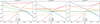Fig. 2. Complete self-similar solutions for three cases (from left to right): (m, n) = (1.3, 2.3),(1.5, 3), and (2, 5). The dimensionless density, velocity, temperature, and mass are shown in blue, orange, green, and red, respectively. The solutions for t < 0 and t > 0 are shown with dashed and solid lines respectively.

3.3. Effective polytropic indices and parameter domain

The effective polytropic indices of the three asymptotes are shown in Fig. 1. We only show n > 1, where the cooling rate scales at least linearly with the internal energy. The red and blue areas correspond to Γ greater and less than unity, respectively. The characteristic values of Γ = 1, Γ = Γ_crit = 4/3, and Γ = γ = 5/3 are marked with white, yellow, and green lines, respectively.

It is possible to infer that for m ≳ 1.5 the central flat region can have slightly decreasing temperature toward the central region with higher density (Γ_i < 1). The freefalling late path always has Γ_l greater than that of the exterior region Γ_e. This can be physically interpreted with the decreased dynamical time, leading to less efficient cooling. There are some special cases: the exterior path is isothermal when m = 1.5, and so is the late path with m = 2.

When cooling is inefficient (i.e., small m and small n values), some combinations can lead to Γ_e > γ. More specifically, this happens when

$$\begin{array}{c}\hfill (n-1)[m+(\gamma -1)n-(\gamma +\frac{1}{2})]<0,\end{array}$$(40)

which corresponds to the region below the green line in the middle panel of Fig. 1. The cooling in the inner region with higher density and higher temperature is not sufficiently efficient compared to the outer region. This situation leads to an apparent polytropic index larger than the adiabatic index that seems to be unphysical at first glance. However, this is derived from the apparent EOS that describes an ensemble of gas instead of the thermal evolution of an individual fluid element. In other words, the actual thermal properties of the gas should be studied along a material line instead of using instantaneous snapshots of density and temperature profiles. This will be detailed further in Sect. 3.5. A similar situation can lead to apparent superadiabaticity Γ_l > γ, which happens when

$$\begin{array}{c}\hfill (n-1)[m+(\gamma -1)n-(\gamma +1)]<0.\end{array}$$(41)

This corresponds to the region below the green line in the right panel of Fig. 1.

Not all combinations of m and n allow the existence of a self-similar solution throughout the whole domain. Constraints such as negative velocity, net cooling, and positive mass, need to be satisfied for physical collapse solutions. These constraints are illustrated in the left panel of Fig. 3, where forbidden zones are color-shaded. The derivations for these conditions are detailed in Appendix D.1. The above-mentioned criteria for solutions at t < 0 and t > 0 are independent, while they must be satisfied simultaneously for solutions to be connected across time zero. If we compare Figs. 1 and 3, we see that superadiabaticity (Γ_l > γ) never occurs in the physically allowed domain of the late path. Γ_i > γ can occur in a narrow band, although this solution is not part of a full solution.

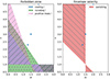Fig. 3. Parameter space analyses. Left: forbidden domain of self-similar solution existence. A complete solution only exists for combinations of m and n in the white area. Right: large-scale velocity behavior. The velocity converges to zero at infinite distance in the shaded zone. The parameters used for the example cases are marked with blue stars.

On the other hand, apparent superadiabaticity can easily occur for the exterior path since there are no physical constraints, although such a solution cannot continue smoothly to ξ ≪ 1. The collapsing cloud is connected to larger scales, where the flow could be converging, static, or expanding. Therefore, conditions in the exterior path do not impose criteria for the existence of solutions. The cloud that has vanishing velocity at infinity can be interpreted as isolated, while that with nonzero velocity can be regarded as embedded in a converging flow. These regimes with vanishing velocity are illustrated in the right panel of Fig. 3 (see derivation in Appendix D.2). It is not possible to tell whether the large-scale velocity is converging or expanding without performing direct numerical simulation, while it is unlikely to have an expanding envelope if the center of the self-similar solution is contracting.

3.4. Evolution in physical coordinates

We transform the self-similar solution back to physical coordinates by assigning a value for Λ₀. The evolution of the profiles are shown in Fig. 4 for m = 1.3 and n = 2.3, while the other two cases can be found in Appendix E. The behavior is basically very similar to what was suggested in previous isothermal and polytropic calculations. The inner flat region shrinks in size and increases in density before time zero, and the freefall onto the central singularity proceeds inside-out. The exterior profile is stationary.

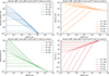Fig. 4. Profiles in physical coordinate with Λ(106 cm−3, 10 K) = 10−26 erg cm−3 s−1, m = 1.3, and n = 2.3. Solutions for t < 0 and t > 0 are presented with dashed and solid lines, respectively. The increasing line thickness corresponds to increasing absolute time.

To obtain some physical insights of the characteristic values, we express

$$\begin{array}{cc}\hfill r& ={A|t|}^{1/a}\xi \hfill \\ \hfill & ={\left(\frac{K_1}{4\pi G}\right)}^{\frac{1-m}{2n-2}}{\left(\frac{k_{\mathrm{B}}}{\mu m_{\mathrm{p}}}\right)}^{\frac{n}{2n-2}}{\left(\frac{\frac{c}{\gamma -1}-d}{{\mathrm{\Lambda }}_0}\right)}^{\frac{1}{2n-2}}{|at|}^{1/a}\xi \hfill \\ \hfill & ={\left(\frac{4\pi G{\rho }_{\mathrm{ref}}}{K_1}\right)}^{\frac{m-1}{2n-2}}{\left(\frac{k_{\mathrm{B}}{T}_{\mathrm{ref}}}{\mu m_{\mathrm{p}}}\right)}^{\frac{n}{2n-2}}{\left(\frac{{\mathrm{\Lambda }}_0{\rho }_{\mathrm{ref}}^{m-1}{T}_{\mathrm{ref}}^n}{\frac{c}{\gamma -1}-d}\right)}^{\frac{-1}{2n-2}}{|\mathit{at}|}^{\frac{2m+2n-5}{2n-2}}\xi ,\hfill \end{array}$$(42)

$$\begin{array}{cc}\hfill M& =4\pi A^{3}B{|t|}^{(3-2a)/a}\mathrm{\Omega }(\xi )\hfill \\ \hfill & =4\pi {\left(\frac{K_1}{4\pi G}\right)}^{\frac{1-3m+2n}{2n-2}}{\left(\frac{k_{\mathrm{B}}}{\mu m_{\mathrm{p}}}\right)}^{\frac{3n}{2n-2}}{\left(\frac{\frac{c}{\gamma -1}-d}{{\mathrm{\Lambda }}_0}\right)}^{\frac{3}{2n-2}}{|\mathit{at}|}^{\frac{-11+6m+2n}{2n-2}}\mathrm{\Omega }(\xi )\hfill \\ \hfill & ={\left(\frac{4\pi G{\rho }_{\mathrm{ref}}}{K_1}\right)}^{\frac{3m-3}{2n-2}}{\left(\frac{k_{\mathrm{B}}{T}_{\mathrm{ref}}}{\mu m_{\mathrm{p}}}\right)}^{\frac{3n}{2n-2}}{\left(\frac{{\mathrm{\Lambda }}_0{\rho }_{\mathrm{ref}}^{m-1}{T}_{\mathrm{ref}}^n}{\frac{c}{\gamma -1}-d}\right)}^{\frac{-3}{2n-2}}{|at|}^{\frac{6m+2n-11}{2n-2}}\frac{K_1}{G}\mathrm{\Omega }(\xi ),\hfill \end{array}$$(43)

where ρ_ref and T_ref are arbitrary reference values. The temporal evolution of central density is solely determined by the combination of m and n, while the temperature, mass, and the physical extent of the inner solution (early interior path and late path) decrease with more effective cooling (larger Λ₀). Due to the power-law dependences on m and n, it is not straightforward to derive characteristic reference values. Nonetheless, under the limits that m is small and n is large, we recover the similarity normalization of the isothermal case (Shu 1977; Whitworth & Summers 1985), where

$$\begin{array}{c}\hfill r\approx c_0|t|\xi ,M\approx \frac{c_0^3|t|}{G}\mathrm{\Omega }(\xi ),\end{array}$$(44)

with $c_0^2=k_{\text{B}}{T}_{\text{ref}}/\mu m_{\text{p}}$. It is also evident from Fig. 1 that when n ≫ 1, all three Γ_A values approach unity irrespective of m.

3.5. Material equation of state

The above-mentioned polytropic indices are relevant for single time frames of a collapsing sphere, which should be compared to resolved observations of a region or a snapshot from a simulation. The results represent an ensemble EOS, or apparent EOS, which is defined with Eq. (29). The effective EOS, or more precisely the temperature-density relation, is shown in Fig. 5 for the three example cases. The early interior path corresponds to a very short segment on these plots since both density and temperature are almost constant. The solution at low density and that at positive time tend very quickly to the power-law asymptotes (described in Sect. 3.1). In particular, the temperature approaches a constant value on the late path for m = 1.5 and on the exterior path for m = 2.

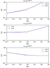Fig. 5. Temperature–density relation for three cases (from top to bottom): (m, n) = (1.3, 2.3), (1.5, 3), and (2, 5). Solutions for t < 0 and t > 0 are shown with dashed and solid lines, respectively. The asymptotic polytropic indices are (Γi, Γe, Γl) = (0.96, 1.15, 1.534), (0.93, 1.0, 1.25), and (0.87, 0.88, 1.0), respectively.

On the other hand, in order to understand the thermodynamical behavior of one single fluid parcel, it is necessary to discuss the material EOS, which is in fact the true EOS,

$$\begin{array}{c}\hfill {\mathrm{\Gamma }}_{\mathrm{M}}-1={\frac{\mathrm{d}logT}{\mathrm{d}log\rho }|}_M=\frac{\mathrm{d}logT/\mathrm{d}t}{\mathrm{d}log\rho /\mathrm{d}t},\end{array}$$(45)

where the material derivative

$$\begin{array}{c}\hfill \frac{\mathrm{d}}{\mathrm{d}t}=\frac{\partial }{\partial t}+u\frac{\partial }{\partial r}=\frac{\partial }{\partial t}-\frac{\xi \mp v}{\mathit{at}}\frac{\partial }{\partial \xi }.\end{array}$$(46)

We can then derive

$$\begin{array}{c}\hfill {\mathrm{\Gamma }}_{\mathrm{M}}=1+\frac{\frac{c}{a}-\frac{\xi \mp v}{a}\frac{{\tau }^{\prime }}{\tau }}{-2-\frac{\xi \mp v}{a}\frac{g^{\prime }}{g}}.\end{array}$$(47)

Inserting the asymptotic solutions previously derived, we can obtain the material polytropic index for the asymptotes. On the early interior path, a fluid parcel follows

$$\begin{array}{c}\hfill {\mathrm{\Gamma }}_{\mathrm{M},\mathrm{i}}\approx 1-\frac{c}{2a}={\mathrm{\Gamma }}_{\mathrm{e}}\end{array}$$(48)

on the T − ρ plane, which is parallel to the exterior path. On the exterior path, the material polytropic index

$$\begin{array}{cc}& {\mathrm{\Gamma }}_{\mathrm{M},\mathrm{e}}\approx 1+\frac{(\frac{c}{2}-1)\frac{{\tau }_{-2}}{{\tau }_{\infty }}\mp c{v}_{\infty }}{(\frac{c}{2}-1)\frac{g_{-2}}{g_{\infty }}\mp d{v}_{\infty }}=\gamma +\frac{c-d(\gamma -1)}{3-a}\frac{g_{\infty }^{m-1}{\tau }_{\infty }^{n-1}}{v_{\infty }},\hfill \end{array}$$(49)

which falls somewhere between Γ_e and Γ_l. We can verify that Γ_M, e < γ in the physical domain of m and n. On the late path, the fluid parcel evolves along the polytrope with index

$$\begin{array}{c}\hfill {\mathrm{\Gamma }}_{\mathrm{M},\mathrm{l}}\approx 1+\frac{2-m}{n-1}={\mathrm{\Gamma }}_{\mathrm{l}},\end{array}$$(50)

which is identical to that of the ensemble EOS. It is sometimes not explicitly stated in the literature whether the apparent or material EOS is used. We discuss and clarify the usage in Appendix F.

The material equation of state can be inferred by tracing the density and temperature evolution at a fixed mass coordinate. Figure 6 shows some examples of the material evolution following enclosed mass M = 1, 10, 100, 1000, 10 000 M_⊙ (gray lines with increasing thickness). Each gray line represents the time evolution of a fluid parcel at a given mass coordinate, in contrast to the spatial profiles at given instants presented with colored lines. When t < 0 the material EOSs at any mass fall on the same line, parallel to the exterior path, and move along Γ_M, i. When a fluid parcel is swept by the inside-out collapse wave, its trajectory turns upward in the T − ρ plane. Finally when entering the freefall at t > 0, the material EOS has the same slope, Γ_M, l, as that of the late path, but with varied absolute values for each mass coordinate.

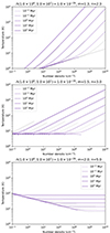Fig. 6. Temperature–density relation snapshots of the three example cases shown in Figs. 4, E.1, and E.2. Solutions for t < 0 and t > 0 are presented with dashed and solid lines, respectively. The colored lines with increasing thickness correspond to increasing absolute time. The gray curves with increasing thickness trace the time evolution of fluid parcels at enclosed mass coordinate M = 1, 10, 100, 1000, 10 000 M⊙.

4. Discussion

4.1. Characteristic timescales

There are several mechanisms that act simultaneously. According to the relative value of the timescales, the physical behavior of the system is thus different. To discuss the various regimes, we evaluate the relevant timescales:

• Freefall timescale: $t_{\mathrm{ff}}=\sqrt{\frac{3\pi }{32G\rho }}$;

• Cooling timescale: $t_{\mathrm{cool}}=\frac{ϵ}{\mathrm{\Lambda }}=\frac{k_{\mathrm{B}}nT}{(\gamma -1)\mathrm{\Lambda }}$;

• Dynamical timescale: $t_{\mathrm{dyn}}=\frac{r}{v}$;

• Pressure timescale: $t_{\mathrm{P}}=\frac{r}{c_{\mathrm{s}}}=r\sqrt{\frac{\mu m_{\mathrm{p}}}{{\mathrm{\Gamma }}_{\mathrm{M}}{k}_{\mathrm{B}}T}}$;

Nishida (1968) has discussed the collapse of a prestellar core by comparing the timescales. When the cooling or heating timescale is significantly smaller than the freefall timescale, the gas contracts or expands very quickly toward the cooling-heating equilibrium until the cooling timescale becomes comparable to the freefall timescale. Subsequently, the gas contracts along the equilibrium t_cool ≈ t_ff.

Consistently found in our work, the collapsing gas always tends to reach a state where t_dyn ∼ t_cool. In a medium with relatively short cooling and heating timescales, this stationary state should occur very close to the equilibrium line between cooling and heating. This temperature is still slightly offset with respect to the equilibrium temperature, with a small net cooling that has a timescale comparable to the dynamical time.

Having obtained the collapse solutions, we can then calculate the relation between the timescales:

$$\begin{array}{cc}& t_{\mathrm{cool}}/t_{\mathrm{ff}}=\frac{1}{(\gamma -1)\pi a{K}_2}\sqrt{\frac{8K_1}{(3-2a)}}{\tau }^{1-n}{g}^{\frac{3}{2}-m}\sqrt{\frac{\xi \mp v}{\xi }};\hfill \end{array}$$(51)

$$\begin{array}{cc}& t_{\mathrm{P}}/t_{\mathrm{ff}}=\frac{1}{\pi }\sqrt{\frac{8K_1}{{\mathrm{\Gamma }}_{\mathrm{M}}(3-2a)}}\sqrt{\frac{\xi g(\xi \mp v)}{\tau }};\hfill \end{array}$$(52)

$$\begin{array}{cc}& t_{\mathrm{dyn}}/t_{\mathrm{ff}}=\frac{1}{\pi }\sqrt{\frac{8K_1}{3-2a}}\frac{\sqrt{\xi g(\xi \mp v)}}{|v|}.\hfill \end{array}$$(53)

On the early interior path, t_P/t_ff scales linearly with the radius, being small near the center, while all other timescales are of the same order of magnitude as the freefall timescale. The small pressure timescale maintains the flat pressure and density profiles of the central region. On the exterior path, all the above-mentioned timescales are maintained with constant ratios. The system therefore reaches a stationary state. On the late path,

$$\begin{array}{c}\hfill t_{\mathrm{P}}/t_{\mathrm{ff}}\propto {\xi }^{-\frac{1}{2}-\frac{3}{4}\frac{m-2}{n-1}}\propto {\xi }^{\frac{8-3m-2n}{4(n-1)}},\end{array}$$(54)

which increases with decreasing radius (cf. the physical parameter domain in Fig. 3). The thermal pressure becomes unimportant as the freefall proceeds. Both t_cool and t_dyn remain in a constant ratio with the freefall time. The difference among the three regimes comes mainly from the different scaling behaviors of the pressure timescale.

4.2. Convective stability

The Schwarzschild instability criterion can be translated into²

$$\begin{array}{c}\hfill {\mathrm{\Gamma }}_A>{\mathrm{\Gamma }}_{\mathrm{M}}.\end{array}$$(55)

The interpretation is straightforward: if the environmental temperature gradient is too steep compared to the material variation (governed by radiation in this context), a perturbation cannot be restored by buoyancy and will lead to convection. This is valid when the local dynamical timescale of the perturbation is larger than the radiation timescale. Otherwise, radiation will not have enough time to act, and the gas polytropic index Γ_M should be replaced with γ. In the physical regime of m and n combinations (cf. Fig. 3), the material polytropic index in always larger than the apparent polytropic index, as can be seen from the expressions of Γ_M in Sect. 3.5 and Fig. 1. If we look at the points where a gray line intercepts a colored line in Fig. 6, their slopes indicate the material and apparent (environment) polytropic indices, respectively. The slope of the gray line is always greater than the colored line, implying that the stability against convection and a perturbed gas parcel always tends to move back to its original position.

4.3. New perspective on the collapse criteria

From energy arguments it can be demonstrated that the effective polytropic index, Γ, of a gas must be smaller than a critical value for collapse to happen. However, instead of defining a critical value of Γ for collapse to occur, we demonstrate in this work that it is physically more relevant to define a cooling function that allows the existence of a collapse solution. The mass positivity condition (Eq. (D.7)) coincides with Γ_e < 4/3, while it is evident that this collapsing envelope could be connected to an inner freefalling region with Γ_l > 4/3. The existence of runaway collapse only requires that Γ_l < γ = 5/3, not 4/3.

5. Conclusions

In this study, we discussed a spherically collapsing gas cloud that follows a parametric cooling law Λ ∝ ρ^mTⁿ. The effective EOS of a cooling and self-gravitating gas can be divided into different regimes according to the relative values of the dynamical and thermal timescales. A self-similar solution is found for such a system, which consists of a central region that is either flat or freefalling before and after the mass singularity formation, and an outer part that is undergoing stationary contraction. This is very similar to other existing collapse solutions.

The distinct feature of the current work is that the effective gas EOS, for the three regimes of the solution, can be directly derived given a parametric cooling function. We derived both the ensemble (apparent) EOS of a collapsing profile snapshot and the material (real) EOS of the fluid parcels within. Instead of examining the effective Γ as the collapse criteria, the cooling function should be used to determine whether the energy can be efficiently evacuated during the collapse process.

The spherically symmetric configuration was discussed in the present manuscript. Nonetheless, on the scales of cloud structure formation, cylindrical collapse, corresponding to filament formation, and plane-parallel geometry, corresponding to colliding flows, should also be of physical interest and worth further investigation. We will continue the calculations in the upcoming work.

Acknowledgments

The author would like to thank the anonymous referee for constructive comments that helped to make the manuscript more concise and comprehensive. This work received financial support of the NSTC (project number 111-2636-M-003-002), and the MOE Yushan Young Fellow program. This work was initiated during the JSPS fellowship in 2020 at Nagoya University.

References

Appendix A: Trivial solution for t < 0

A trivial solution can be identified when K₁ = K₀ = d²/6:

$$\begin{array}{c}\hfill g(\xi )=1,v(\xi )=\frac{d}{3}\xi ,\tau (\xi )=1.\end{array}$$(A.1)

This solution describes the homologous collapse of a flat structure that extends to infinity, and is valid only for t < 0. For this solution Γ is undetermined since both g and τ are constant. It is of less interest in the current context, and thus we do not discuss it in detail.

Appendix B: Derivation of the asymptotic solutions and the sonic point

B.1. Early interior path, t < 0, ξ ≪ 1

We presume the polynomial series for the centrally flat profiles before the mass singularity formation:

$$\begin{array}{cc}\hfill g& =1+g_1\xi +g_2{\xi }^2+\mathcal{O}\left({\xi }^3\right);\hfill \end{array}$$(B.1)

$$\begin{array}{cc}\hfill v& =v_0+v_1\xi +v_2{\xi }^2+v_3{\xi }^3+\mathcal{O}\left({\xi }^4\right);\hfill \end{array}$$(B.2)

$$\begin{array}{cc}\hfill \tau & =1+{\tau }_1\xi +{\tau }_2{\xi }^2+\mathcal{O}\left({\xi }^3\right).\hfill \end{array}$$(B.3)

Since A and B are free parameters, we can thus choose a scaling such that the leading terms of g and τ are both unity. Physical boundary conditions require

$$\begin{array}{c}\hfill g^{\prime }(0)=0,v(0)=0,{\tau }^{\prime }(0)=0,\end{array}$$(B.4)

which implies the absence of singularity at the origin. Substituting into the equations, it is easily found that

$$\begin{array}{c}\hfill g_1=v_0=v_2={\tau }_1=0.\end{array}$$(B.5)

In short, all odd-order terms of g and τ and even-order terms of v should vanish for symmetry reasons. The asymptotic solutions simplify to

$$\begin{array}{cc}\hfill g& =1+g_2{\xi }^2,v=v_1\xi +v_3{\xi }^3,\tau =1+{\tau }_2{\xi }^2,\hfill \end{array}$$(B.6)

$$\begin{array}{cc}\hfill \mathrm{\Omega }& =(\frac{{\xi }^3}{3}+\frac{g_2{\xi }^5}{5})=\frac{(1+v_1)}{(3-2a)}{\xi }^3+\frac{(g_2+g_2{v}_1+v_3)}{(3-2a)}{\xi }^5.\hfill \end{array}$$(B.7)

Inserting into the governing equation set, we obtain

$$\begin{array}{cc}\hfill v_1& =\frac{d}{3}=\frac{4}{3}\frac{n-1}{5-2m-2n};\hfill \end{array}$$(B.8)

$$\begin{array}{cc}\hfill 0& =2(v_1+1)g_2+5v_3;\hfill \end{array}$$(B.9)

$$\begin{array}{cc}\hfill g_2+{\tau }_2& =\frac{v_1^2}{4}-\frac{K_1}{3-2a}\frac{v_1+1}{2};\hfill \end{array}$$(B.10)

$$\begin{array}{cc}\hfill K_2& =\frac{c}{\gamma -1}-d;\hfill \end{array}$$(B.11)

$$\begin{array}{cc}\hfill g_2& =(\frac{v_1^2}{4}-\frac{K_1}{3-2a}\frac{v_1+1}{2})\frac{2\frac{v_1+1}{\gamma -1}+(n-1)K_2}{2\gamma \frac{v_1+1}{\gamma -1}+(n-m)K_2}.\hfill \end{array}$$(B.12)

It should be noted that K₁ determines the sign and amplitude of g₂. Fixing the temperature leading term τ₀ = 1 is equivalent to fixing the value of K₂. The variation of τ₀ and K₂ leads to rescaling of the system, which corresponds to exactly the same solution when transformed back into physical units.

The effective polytropic index can be derived by inserting the asymptotes into Eq. (29), which yields

$$\begin{array}{c}\hfill {\tau }_2=g_2({\mathrm{\Gamma }}_{\mathrm{i}}-1).\end{array}$$(B.13)

There are two conditions that give Γ_i = γ. One is when (n − m)/(n − 1) = γ, and the other is when (c − (γ − 1)d) = 0. The conditions translate respectively to

$$\begin{array}{cc}\hfill m+(\gamma -1)n& =\gamma ,\mathrm{and}\hfill \end{array}$$(B.14)

$$\begin{array}{cc}\hfill m+(\gamma -1)n& =\gamma +1/2.\hfill \end{array}$$(B.15)

For γ = 5/3, the first condition gives 3m + 2n = 5 and the second 6m + 4n = 13. The denominator vanishes on the curve

$$\begin{array}{c}\hfill m=\frac{5}{2}-\frac{2n}{3}-\frac{1}{3n},\end{array}$$(B.16)

where the sign of Γ_i changes from positive to negative infinity on the two sides. We note that this polytropic index value is independent of the choice of A and B. When K₁ = K₀ = d²/6, the trivial solution is recovered.

B.2. Exterior path, ξ ≫ 1

The asymptotic solution at large distances, or close to the mass singularity formation epoch, can be expanded in power-law series

$$\begin{array}{cc}\hfill v& =v_{\infty }{\xi }^{c/2}\pm v_{-2}{\xi }^{c-1}+\mathcal{O}\left({\xi }^{3c/2-2}\right),\hfill \end{array}$$(B.17)

$$\begin{array}{cc}\hfill g& =g_{\infty }{\xi }^{c-2}\pm g_{-2}{\xi }^{3c/2-3}+\mathcal{O}\left({\xi }^{2c-4}\right),\hfill \end{array}$$(B.18)

$$\begin{array}{cc}\hfill \tau & ={\tau }_{\infty }{\xi }^c\pm {\tau }_{-2}{\xi }^{3c/2-1}+\mathcal{O}\left({\xi }^{2c-2}\right),\hfill \end{array}$$(B.19)

where the highest order constants are to be determined by numerical integration if one wishes to connect the solutions smoothly to ξ ≪ 1. The lower order terms follow

$$\begin{array}{cc}\hfill (\frac{c}{2}-1)g_{-2}& =\frac{3}{2}c{v}_{\infty }{g}_{\infty },\hfill \end{array}$$(B.20)

$$\begin{array}{cc}\hfill (\frac{c}{2}-1)v_{-2}& =\frac{c}{2}{v}_{\infty }^2+2(c-1){\tau }_{\infty }+K_1{g}_{\infty },\hfill \end{array}$$(B.21)

$$\begin{array}{cc}\hfill (\frac{c}{2}-1)\frac{{\tau }_{-2}}{\gamma -1}& =(\frac{c}{\gamma -1}+b+2)v_{\infty }{\tau }_{\infty }+K_2{g}_{\infty }^{m-1}{\tau }_{\infty }^n.\hfill \end{array}$$(B.22)

B.3. Alternative asymptotes for ξ ≫ 1

The asymptotic solution at large distances or close to the mass singularity formation time has an alternative form with nonvanishing velocity

$$\begin{array}{cc}\hfill v& =\mp \frac{d}{3}\xi ,\hfill \end{array}$$(B.23)

$$\begin{array}{cc}\hfill g& =g_{\infty },\hfill \end{array}$$(B.24)

$$\begin{array}{cc}\hfill \tau & ={\tau }_{\infty },\hfill \end{array}$$(B.25)

where

$$\begin{array}{cc}\hfill g_{\infty }& =\frac{d^2}{6K_1(3+d)},\hfill \end{array}$$(B.26)

$$\begin{array}{cc}\hfill {\tau }_{\infty }^{n-1}& =\pm \frac{c(\gamma -2)/(\gamma -1)-2}{K_2{g}_{\infty }^{m-1}}.\hfill \end{array}$$(B.27)

This asymptotic solution exists for opposite domains of m-n combination for t → 0⁻ and t → 0⁺. Therefore, the solutions cannot be connected smoothly across time zero.

B.4. The sonic point (surface)

When writing the equation set as linear combinations of the derivatives, some algebraic manipulation yields

$$\begin{array}{c}\hfill g^{\prime }=\frac{{\mathrm{\Delta }}_1}{\mathrm{\Delta }},v^{\prime }=\frac{{\mathrm{\Delta }}_2}{\mathrm{\Delta }},{\tau }^{\prime }=\frac{{\mathrm{\Delta }}_3}{\mathrm{\Delta }},\end{array}$$(B.28)

where

$$\begin{array}{c}\hfill \mathrm{\Delta }={(v\mp \xi )}^2-\gamma \tau \end{array}$$(B.29)

is the determinant of the system, and

$$\begin{array}{cc}\hfill {\mathrm{\Delta }}_2& =\pm \frac{K_1}{3-2a}g{(v\mp \xi )}^2\mp bv(v\mp \xi )\pm (c+d)\tau \hfill \end{array}$$(B.30)

$$\begin{array}{cc}& +\frac{2\gamma v\tau }{\xi }+K_2(\gamma -1)g^{m-1}{\tau }^n;\hfill \\ \hfill {\mathrm{\Delta }}_1& =-\frac{g(\pm d+\frac{2v}{\xi })}{(v\mp \xi )}\mathrm{\Delta }-\frac{g}{(v\mp \xi )}{\mathrm{\Delta }}_2;\hfill \end{array}$$(B.31)

$$\begin{array}{cc}\hfill {\mathrm{\Delta }}_3& =-\frac{\pm c\tau +\frac{2(\gamma -1)\tau v}{\xi }+K_2{g}^{m-1}{\tau }^n(\gamma -1)}{(v\mp \xi )}\mathrm{\Delta }-\frac{\tau (\gamma -1)}{(v\mp \xi )}{\mathrm{\Delta }}_2.\hfill \end{array}$$(B.32)

The criterion Δ(g, v, τ) = 0 defines a sonic surface. The solutions with t > 0 does not pass through through the sonic surface. On the other hand, for the solutions with t < 0 to pass smoothly through the sonic surface, the conditions

$$\begin{array}{c}\hfill \mathrm{\Delta }={\mathrm{\Delta }}_2=0\end{array}$$(B.33)

must be satisfied simultaneously on the sonic point, where the solution intercepts the sonic surface, and

$$\begin{array}{c}\hfill {\mathrm{\Delta }}_1={\mathrm{\Delta }}_3=0\end{array}$$(B.34)

also holds through linear dependance.

There are two types of solution that can pass through the sonic point smoothly. The first type is the trivial solution where the density and the temperature both remain constant (Appendix A). The other valid value of K₁ must be inferred by performing the shooting method toward the sonic point with numerical integration. Depending on m and n, sometimes K₁ < K₀ and leads to increasing density with increasing distance from the center. In this case the exterior solution crosses the sonic surface again, while not satisfying Eq. (B.33). If we somehow relax the continuity condition at the sonic point, it is then still possible to find a pair of early interior path and exterior path solutions that are connected through a shock. Due to its complexity, we do not study the detailed properties of the sonic point in the present work.

B.5. Time reversibility

The gas might be subject to heating at low density and low temperature, while the current study does not consider the heating mechanism. The effect of heating can be easily obtained by changing the sign of the cooling term. With a transformation of the time coordinate t → −t, this results in an expansion solution that has exactly the same effective polytropic indices.

For the monoatomic gas with γ = 5/3 considered in this study, a self-similar collapse solution can only exist when cooling is considered; we recall that the critical value in spherical geometry is 4/3. If heating is present instead, the thermal energy must exceed the gravitational energy at some moment, and thus the collapse cannot continue infinitely. On the other hand, the present self-similar solution remains valid if the sign of the entire system is reversed.

Appendix C: Thermal behavior of gas in simulations with cooling

We compared our results to the numerical results in the literature. Since the current model is a generic model that only requires knowing the cooling function, it can therefore be easily applied to various cooling mechanisms.

C.1. Regular ISM

Tarafdar et al. (1985) simulated the thermal evolution of a collapsing cloud with a cooling chemical network. Lesaffre et al. (2005) also performed 1D spherical collapse simulation coupled to a chemical network and radiation, while solving the dust temperature explicitly. The evolution of density, temperature, and velocity profiles obtained in these two studies is very similar to our self-similar solution with m ≈ 2 before time zero (see Fig. 2 in Tarafdar et al. 1985). The central region has almost flat density and temperature profiles and undergoes homologous collapse. The size of this central region shrinks and the temperature decreases with time, while the envelope is stationary and the velocity vanishes at infinity.

Lesaffre et al. (2005) found a density profile with slope shallower than −2 and a decreasing temperature profile toward the center when cooling is considered. This is exactly reproduced with the current solution with m > 3/2. However, our solution is not applicable to their results when the central density reaches ∼10⁹cm⁻³, where the cooling becomes optically thick. Since some of the major chemical reactions in a star-forming core have comparable timescales to that of the collapse, correctly calculating the temperature is important for out-of-equilibrium chemistry (e.g., Pagani et al. 2013). However, a full 3D hydrodynamical simulation with a complete chemical network and radiative transfer is still numerically challenging at present.

C.2. Primordial ISM

Yoshida et al. (2006) used the cooling model for primordial gas (Abel et al. 1997; Galli & Palla 1998), with cooling dominated by hydrogen molecules. Molecular hydrogen being the major coolant, m ≈ 2 for the optically thin low density gas and m ≈ 1 at higher densities, and a steep temperature dependence gives n > 1. Our model explains why the effective Γ switches from below unity to above at density ≈10³ − 10⁴ cm⁻³ in their Fig. 3. At densities above ≈10¹⁴ cm⁻³, the cooling is dominated by the collision-induced emission and follows m ≈ 1, giving Γ > 1.

At densities of around 10⁹ − 10¹¹ cm⁻³, the rapidly increasing molecular fraction leads to values of m that are significantly larger than unity since the cooling rate depends on the H₂ number density rather than the total number density, which is dominated by hydrogen atoms. Also shown in the simulations by Clark et al. (2011, their Fig. 11) is that the molecular fraction increases roughly linearly with density. Consequently, m ≈ 2, and the effective Γ is slightly lower than unity.

Greif et al. (2011) used the molecular hydrogen cooling with slightly different prescriptions. They performed cosmological simulations and analyzed some minihaloes formed within. At very low density < 1 cm⁻³ the gas heats up adiabatically. After the cooling becomes effective, the behavior at density < 10⁸ cm⁻³ is very similar to that in Yoshida et al. (2006). Interestingly, all minihaloes do not behave identically, and the prolonged HD cooling maintains the temperature at ≈200K in the density range 10⁴ − 10⁸ cm⁻³. This is probably the result of the combination between HD cooling with intrinsically m ≈ 1.5 at density and temperature slightly below values where LTE can be reached (Flower & Le Bourlot 2000) and the HD enhancement at low temperature (McGreer & Bryan 2008).

O’Shea & Norman (2007) performed cosmological simulations for an ensemble of haloes. They found that at higher redshifts, a higher environmental temperature leads to a higher H₂ fraction. This results in haloes with lower central temperature and lower mass accretion rates at comparable central density. These findings are exactly accounted for by our solution, as shown in Eqs. (15) and (16), due to larger Λ₀ value in Eq. (27). Our model also yields a smaller central density plateau under the condition shown in Eq. (14), which is seen in their Fig. 11.

Appendix D: Parameter space

D.1. Physical regime

On the early interior path, the contracting condition for the center, v₁/a < 0, is automatically satisfied. The cooling condition requires K₂/a > 0 (cf. Eq. (26)). This is equivalent to

$$\begin{array}{c}\hfill (n-1)[m+(\gamma -1)n-(\gamma +\frac{1}{2})]>0,\end{array}$$(D.1)

or alternatively,

$$\begin{array}{c}\hfill (n-1)(6m+4n-13)>0,\mathrm{for}\gamma =5/3.\end{array}$$(D.2)

The forbidden parameter space is shaded in blue with dots in the left panel of Fig. 3.

On the late path, the existence of the runaway solution requires the positivity of Eq. (37), which means that

$$\begin{array}{c}\hfill a{K}_2(\frac{1}{\gamma -1}\frac{m-2}{n-1}+1)>0,\end{array}$$(D.3)

which yields

$$\begin{array}{c}\hfill (n-1)[m+(\gamma -1)n-(\gamma +\frac{1}{2})][m+(\gamma -1)n-(\gamma +1)]>0,\end{array}$$(D.4)

or alternatively,

$$\begin{array}{c}\hfill (n-1)(6m+4n-13)(3m+2n-8)>0,\mathrm{for}\gamma =5/3.\end{array}$$(D.5)

This forbidden parameter space is shaded in green with circles in Fig. 3 (left panel). Another mass positivity criterion from Eqs. (24), (34), and (35) for a collapsing late path solution requires

$$\begin{array}{c}\hfill a(3-2a)>0,\end{array}$$(D.6)

which translates into

$$\begin{array}{c}\hfill (n-1)(6m+2n-11)>0.\end{array}$$(D.7)

The forbidden parameter space is shaded in pink with slashes in Fig. 3 (left panel). The late path solution should satisfy Eqs. (D.4) and (D.7) at the same time.

D.2. Large-scale behavior

There are no physical constraints on the cooling parameters at large scales. However, the parameter space is separated into regimes, where the velocity vanishes at infinity or not. Vanishing velocity at infinite distance requires c < 0, which yields

$$\begin{array}{c}\hfill (2m+2n-5)(2m-3)<0,\end{array}$$(D.8)

which can be interpreted as isolated or accreting clouds. Depending on the large-scale behavior, the cloud can be interpreted to be isolated or connected to a converging flow.

Appendix E: Evolution in physical coordinates

Profiles of density, velocity, temperature, and enclosed mass are plotted at several time frames. They are presented in Figs. E.1 and E.2 for two cases: m = 1.5 and n = 3, and m = 2 and n = 5.

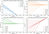Fig. E.1. Profiles in physical coordinates with Λ(106cm−3, 10K) = 10−26 erg cm−3s−1, m = 1.5, and n = 3. Solutions for t < 0 and t > 0 are shown with dashed and solid lines, respectively. The increasing line thickness corresponds to increasing absolute time.

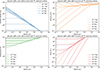Fig. E.2. Profiles in physical coordinates with Λ(106cm−3, 10K) = 10−26 erg cm−3s−1, m = 2, and n = 5. Solutions for t < 0 and t > 0 are shown with dashed and solid lines, respectively. The increasing line thickness corresponds to increasing absolute time.

Appendix F: Ambiguity in the usage of the polytropic Γ

As an extension to the self-similar solution of an isothermal gas (Shu 1977; Hunter 1977; Whitworth & Summers 1985), Yahil (1983) studied the self-similar solution of a polytropic gas with³

$$\begin{array}{c}\hfill P=K{\rho }^{\mathrm{\Gamma }},\end{array}$$(F.1)

where K is a constant. This EOS fixes the trajectory of all fluid elements onto a single straight line on the log T − log ρ plane (i.e., Γ ≡ Γ_A = Γ_M). Suto & Silk (1988) further generalized this calculation to a gas that follows

$$\begin{array}{c}\hfill P=K(t){\rho }^{\mathrm{\Gamma }},\end{array}$$(F.2)

where K is a function of time. This solution describes an ensemble of gas that falls on a straight line on the log T − log ρ plane with fixed slope, while the exact position of this line evolves with time. A constant K value being a special case, the actual trajectory of gas on the log T − log ρ plane is generally different from the gas ensemble distribution: Γ ≡ Γ_A ≠ Γ_M. In some of their solutions, the gas has to be either cooled or heated in different regions to maintain this overall polytropic appearance.

Murakami et al. (2004) discussed a similar problem to the present study, where the gas has an intrinsic adiabatic index γ and is cooled explicitly with a prescribed cooling function. They used the radiative diffusion as the relevant cooling mechanism in the optically thick regime. They defined

$$\begin{array}{c}\hfill \mathrm{\Gamma }=\gamma -\frac{\gamma -1}{\mathrm{Pe}},\text{where}\mathrm{Pe}\equiv \frac{|p\mathrm{\nabla }·u|}{|\mathrm{\nabla }·q|}\end{array}$$(F.3)

is the Péclet number. This is the definition of the material polytropic index, which describes the thermal behavior of a fluid element that heats up during compression, while some of the energy is lost through radiative diffusion. The thus derived polytropic index, Γ ≡ Γ_M, can be compared to, for example, the evolution of the central region of the first Larson core. While not explicitly stated in their work, they also derived the apparent polytropic index, which is smaller than the material polytropic index.

In the present context, we studied the radiative cooling process in the optically thin regime, with a parameterization as a power-law function of density and temperature. This regime is more relevant for the collapse and structure formation at molecular cloud scales. We demonstrated that the instantaneous temperature and density profiles of a collapsing cloud can exhibit an apparent polytropic index different from that derived from the temporal evolution of the overall (or local) cloud properties.

All Tables

All Figures

Fig. 1. Apparent polytropic indices Γi, Γe, and Γl as functions of m and n. The critical values of 1, 4/3, and 5/3 are marked with white, yellow, and green contours, respectively. In regimes shown in red, the gas temperature increases with increasing density. In regimes shown in blue, the opposite happens. The values of Γ are shown irrespectively of the existence of a collapse solution, while the physical domain is shown in Fig. 3.

In the text

	Fig. 2. Complete self-similar solutions for three cases (from left to right): (m, n) = (1.3, 2.3),(1.5, 3), and (2, 5). The dimensionless density, velocity, temperature, and mass are shown in blue, orange, green, and red, respectively. The solutions for t < 0 and t > 0 are shown with dashed and solid lines respectively.
In the text

	Fig. 3. Parameter space analyses. Left: forbidden domain of self-similar solution existence. A complete solution only exists for combinations of m and n in the white area. Right: large-scale velocity behavior. The velocity converges to zero at infinite distance in the shaded zone. The parameters used for the example cases are marked with blue stars.
In the text

	Fig. 4. Profiles in physical coordinate with Λ(106 cm−3, 10 K) = 10−26 erg cm−3 s−1, m = 1.3, and n = 2.3. Solutions for t < 0 and t > 0 are presented with dashed and solid lines, respectively. The increasing line thickness corresponds to increasing absolute time.
In the text

	Fig. 5. Temperature–density relation for three cases (from top to bottom): (m, n) = (1.3, 2.3), (1.5, 3), and (2, 5). Solutions for t < 0 and t > 0 are shown with dashed and solid lines, respectively. The asymptotic polytropic indices are (Γi, Γe, Γl) = (0.96, 1.15, 1.534), (0.93, 1.0, 1.25), and (0.87, 0.88, 1.0), respectively.
In the text

Fig. 6. Temperature–density relation snapshots of the three example cases shown in Figs. 4, E.1, and E.2. Solutions for t < 0 and t > 0 are presented with dashed and solid lines, respectively. The colored lines with increasing thickness correspond to increasing absolute time. The gray curves with increasing thickness trace the time evolution of fluid parcels at enclosed mass coordinate M = 1, 10, 100, 1000, 10 000 M⊙.

In the text

	Fig. E.1. Profiles in physical coordinates with Λ(106cm−3, 10K) = 10−26 erg cm−3s−1, m = 1.5, and n = 3. Solutions for t < 0 and t > 0 are shown with dashed and solid lines, respectively. The increasing line thickness corresponds to increasing absolute time.
In the text

	Fig. E.2. Profiles in physical coordinates with Λ(106cm−3, 10K) = 10−26 erg cm−3s−1, m = 2, and n = 5. Solutions for t < 0 and t > 0 are shown with dashed and solid lines, respectively. The increasing line thickness corresponds to increasing absolute time.
In the text

References

- Abel, T., Anninos, P., Zhang, Y., & Norman, M. L. 1997, New Astron., 2, 181 [NASA ADS] [CrossRef] [Google Scholar]
- Boland, W., & de Jong, T. 1984, A&A, 134, 87 [NASA ADS] [Google Scholar]
- Clark, P. C., Glover, S. C. O., Klessen, R. S., & Bromm, V. 2011, ApJ, 727, 110 [NASA ADS] [CrossRef] [Google Scholar]
- Disney, M. J., McNally, D., & Wright, A. E. 1969, MNRAS, 146, 123 [NASA ADS] [CrossRef] [Google Scholar]
- Flower, D. R., Le Bourlot, J., & Pineau des Forêts, G., & Roueff, E., 2000, MNRAS, 314, 753 [NASA ADS] [CrossRef] [Google Scholar]
- Galli, D., & Palla, F. 1998, A&A, 335, 403 [NASA ADS] [Google Scholar]
- Goldsmith, P. F. 2001, ApJ, 557, 736 [Google Scholar]
- Greif, T. H., Springel, V., White, S. D. M., et al. 2011, ApJ, 737, 75 [NASA ADS] [CrossRef] [Google Scholar]
- Hollenbach, D., & McKee, C. F. 1979, ApJS, 41, 555 [Google Scholar]
- Hunter, C. 1977, ApJ, 218, 834 [NASA ADS] [CrossRef] [Google Scholar]
- Hunter, J. H. Jr. 1969, MNRAS, 142, 473 [NASA ADS] [CrossRef] [Google Scholar]
- Larson, R. B. 1973a, ARA&A, 11, 219 [NASA ADS] [CrossRef] [Google Scholar]
- Larson, R. B. 1973b, Fund. Cosmic. Phys., 1, 1 [NASA ADS] [Google Scholar]
- Larson, R. B. 1985, MNRAS, 214, 379 [NASA ADS] [Google Scholar]
- Lesaffre, P., Belloche, A., Chièze, J. P., & André, P. 2005, A&A, 443, 961 [NASA ADS] [CrossRef] [EDP Sciences] [Google Scholar]
- McGreer, I. D., & Bryan, G. L. 2008, ApJ, 685, 8 [CrossRef] [Google Scholar]
- Murakami, M., Nishihara, K., & Hanawa, T. 2004, ApJ, 607, 879 [NASA ADS] [CrossRef] [Google Scholar]
- Myers, P. C. 1978, ApJ, 225, 380 [NASA ADS] [CrossRef] [Google Scholar]
- Neufeld, D. A., & Kaufman, M. J. 1993, ApJ, 418, 263 [NASA ADS] [CrossRef] [Google Scholar]
- Neufeld, D. A., Lepp, S., & Melnick, G. J. 1995, ApJS, 100, 132 [Google Scholar]
- Nishida, M. 1968, PASJ, 20, 162 [NASA ADS] [Google Scholar]
- Omukai, K. 2001, ApJ, 546, 635 [NASA ADS] [CrossRef] [Google Scholar]
- O’Shea, B. W., & Norman, M. L. 2007, ApJ, 654, 66 [CrossRef] [Google Scholar]
- Pagani, L., Lesaffre, P., Jorfi, M., et al. 2013, A&A, 551, A38 [NASA ADS] [CrossRef] [EDP Sciences] [Google Scholar]
- Shu, F. H. 1977, ApJ, 214, 488 [Google Scholar]
- Suto, Y., & Silk, J. 1988, ApJ, 326, 527 [CrossRef] [Google Scholar]
- Tarafdar, S. P., Prasad, S. S., Huntress, W. T. Jr., Villere, K. R., & Black, D. C. 1985, ApJ, 289, 220 [NASA ADS] [CrossRef] [Google Scholar]
- Whitworth, A., & Summers, D. 1985, MNRAS, 214, 1 [Google Scholar]
- Yahil, A. 1983, ApJ, 265, 1047 [NASA ADS] [CrossRef] [Google Scholar]
- Yoshida, N., Omukai, K., Hernquist, L., & Abel, T. 2006, ApJ, 652, 6 [NASA ADS] [CrossRef] [Google Scholar]