| Issue |
A&A
Volume 684, April 2024
|
|
|---|---|---|
| Article Number | A10 | |
| Number of page(s) | 18 | |
| Section | Stellar structure and evolution | |
| DOI | https://doi.org/10.1051/0004-6361/202346346 | |
| Published online | 29 March 2024 | |
Three-dimensional time-dependent convection model for asteroseismology
I. Mathematical model
1
Space Sciences, Technologies and Astrophysics Research (STAR) Institute, Université de Liège, Allée du Six-Août 19, 4000 Liège, Belgium
e-mail: This email address is being protected from spambots. You need JavaScript enabled to view it.
2
Observatoire de Genève, Université de Genève, Ch. Pegasi 51, 1290 Sauverny, Switzerland
3
Zentrum für Astronomie der Universität Heidelberg, Landessternwarte, Königstuhl 12, 69117 Heidelberg, Germany
Received:
7
March
2023
Accepted:
31
October
2023
Abstract
Context. Due to an ill-depicting model of the convective layers below the photosphere in 1D stellar models (structural contribution) and/or a misrepresentation of the coupling between convection and oscillations (modal contribution), a well-known deviation appears between observed and theoretical frequencies, which grows towards high frequencies; the so-called surface effects. While satisfying solutions have been found regarding the structural contribution, the accurate modeling of the modal effect still represents a challenge. Alongside the frequency, the interaction between convection and oscillations also impacts the damping rate of the modes and forms an important part of the driving mechanism behind the stellar oscillations of low-mass stars. With increasing observational capabilities at our disposal with Kepler and TESS, shortcomings in modeling constitute the main limitation to accurate seismic probing of solar-like and red giant stars.
Aims. We present the formalism of an approach that changes the current paradigm by addressing three-dimensional space. This new formalism consists in an original nonadiabatic 3D time-dependent convection model for asteroseismology.
Methods. We aim to keep the entire 3D structure of the astrophysical flow in these superficial layers in order to fully account for the nature of turbulence in our model via the use of advanced hydrodynamic simulation. We use the perturbative approach and introduce a spectral decomposition approach that results in an entirely new formalism describing standing waves in 3D. This formalism is set to solve the quasi-radial global nonadiabatic oscillation equations in a full 3D framework.
Results. Based on physical assumptions, we establish an eigenvalue problem describing the 3D quasi-radial global nonadiabatic stellar oscillation. We also provide a prescription for its numerical resolution alongside a proposed iteration method for our formalism. Finally, we derive the peculiar 3D work integral and establish the expression of the damping rate. We show how our formalism offers the possibility to probe the complex structure of stars and is able to precisely locate regions of the driving and damping of the modes as well as their physical origin.
Key words: asteroseismology / convection / methods: numerical / stars: oscillations
© The Authors 2024
 Open Access article, published by EDP Sciences, under the terms of the Creative Commons Attribution License (https://creativecommons.org/licenses/by/4.0), which permits unrestricted use, distribution, and reproduction in any medium, provided the original work is properly cited.
This article is published in open access under the Subscribe to Open model. This email address is being protected from spambots. You need JavaScript enabled to view it. to support open access publication.
1. Introduction
Comparisons between the first asteroseismic models and solar surveys revealed a deviation between theoretical and observational eigenfrequencies, which affected modes of various degrees. These deviations were attributed to the presence of a highly turbulent region in the superficial layer of the Sun. The interaction or coupling between the stellar oscillations and the turbulent convective motion has several consequences. A major consequence are the discrepancies between theory and observations regarding the eigenfrequencies of stellar oscillations, referred to as “surface effects,” which are directly linked to the presence of this superficial convective zone (Dziembowski et al. 1988; Christensen-Dalsgaard et al. 1996; Rosenthal et al. 1999). They are not solely related to the Sun, but affect cold stars with a convective region in their superficial layer (e.g., low-mass main sequence stars and red giant stars). These discrepancies constitute an important limitation in accurate seismic probing of those stars.
Multiple attempts have been made to correct the surfaces effects. On one hand, the structural impact has been modeled using patched models followed by empirical laws to account for the surface effects (Kjeldsen et al. 2008; Ball & Gizon 2014; Sonoi et al. 2015; Trampedach et al. 2017). After computing the adiabatic frequencies of the patched model, free parameters in the empirical laws had to be calibrated or optimized to fit the observations.
On the other hand, the modal impact is processed via the time-dependent convection models based on perturbation of the mixing-length approach for turbulence (Unno 1967; Gough 1977). These latter models (e.g., Gabriel et al. 1975; Houdek 1996; Grigahcène et al. 2005; Sonoi et al. 2017; Houdek et al. 2017, 2019) suffer from the underlying hypotheses behind the mixing-length theory (MLT) and their one-dimensional approach of the problematic (along the radial direction of the star). In the MLT, the turbulent cascade is reduced to a single scale, the mixing length, leading to misrepresentation of turbulent characteristics such as the turbulent pressure. Furthermore, the actual coupling occurs over the entire turbulent spectrum, which possesses features that vary from one region to another (downflows or upflows). Due to horizontal averages, those MLT models are dependent on a closure equation for the Reynolds stress and rely on free parameters – the calibration of which is not always physical – to account for all the features erased by the averaging process. More complex analytical approaches beyond the mixing length have been proposed; these include the use of Reynolds stress models (Xiong et al. 2000), but these suffer from similar drawbacks. Another family of models is based on the use of stellar atmosphere simulation for a direct measure of the mode line widths and damping rates (Nordlund & Stein 2001; Stein & Nordlund 2001; Belkacem et al. 2019; Zhou et al. 2020). As a consequence of the boundary conditions used in the hydrodynamic simulations, normal modes appear to be present in the simulation box in addition to the turbulent acoustic noise. The properties of the normal modes are then examined in order to study the mode physics. However, there are several downsides to studying modes present in a simulation box. Distinguishing those normal modes from convective fluctuations in the simulation box requires a very long simulation of several tens of hours or days and the normal modes identified actually correspond to modes of the box and not to global modes of the star. Therefore, due to the relative difference between the size of the simulation box and the star, the inertia of those modes is much smaller than global stellar modes, which leads to the obtention of modes of a much larger amplitude than those observed. The physics behind those modes is modified compared to reality; for example, nonlinearities resulting from their excessive amplitude could be responsible for an increased importance of certain physical mechanisms, such as the role of dissipation of turbulent kinetic energy in this frame.
In solar-like stars, the mechanism behind their oscillations is the stochastic excitation and damping induced by the turbulence around the photosphere of the star. The coupling between convection and oscillation impacts the energetics of the oscillations, not only in the stars affected by surface effects but also in others such as white dwarfs (Van Grootel et al. 2012), γ Dor, and δ Scuti stars (Dupret et al. 2005). Therefore, the damping of the modes is also directly related to turbulence. Several attempts have been made to model the driving (e.g., Goldreich & Keeley 1977a,b; Samadi & Goupil 2001; Chaplin et al. 2005; Belkacem et al. 2006, 2008, 2010) and damping (e.g., Goldreich & Kumar 1991; Grigahcène et al. 2005; Dupret et al. 2006; Belkacem et al. 2012) of the modes but these suffer the same limitations as the attempts to model surface effects. Moreover, damping models are often computed and adjusted via different methods from those used to deal with surface effects models, which constitutes an anomaly in itself, as both are related in the same manner to the convective motion in the superficial layer of the star; more details regarding the modal effect of turbulence are found in reviews by Houdek & Dupret (2015) and Samadi et al. (2015).
Looking solely at the structure of turbulence is an extremely challenging topic. This is especially stressed in the stellar astrophysical context, with turbulent flows with Reynolds numbers of around 1010 and a very large spectrum of space- and timescales. For those reasons, the first numerical simulations of turbulent flows relied on oversimplification, with models such as the Reynolds-averaged Navier-Stokes (RANS), in which the well-known Prandtl mixing length can be used as a closure equation. However, in recent decades, tremendous progress has been made in computational fluid dynamics with the rise of the Large Eddy Simulation (LES). These simulations are able to solve the Navier-Stokes equations down to a spatial limit, the smallest resolved length scale. These improvements in turbulence modeling also benefit stellar flows (Schmidt 2015; Kupka & Muthsam 2017). For instance, a state-of-the-art LES for stellar surface convection, called “COnservative COde for the COmputation of COmpressible COnvection in a BOx of L Dimensions with l = 2,3” (CO5BOLD), can be used to study convection in solar-type stars, red supergiants, substellar objects, and white dwarfs (Freytag et al. 2012).
As mentioned above, the interaction between convection and stellar oscillations, the modal effect of turbulence, is still an open question in asteroseismology. Despite improvements brought to stellar oscillations models, the current approaches have reached limits regarding questions as to the impact of convection, whether that be in terms of surface effects or damping of the mode. Even with the most recent models based on hydrodynamic simulations, the corrections of the surface effects are unsatisfactory and the damping remains poorly understood. In the current time-dependent convection models, the excitation of the modes, for instance in the γ Dor (Dupret et al. 2005) and white dwarfs (Van Grootel et al. 2012), is not in agreement with the observations and therefore requires further investigation. These points still constitute the main limitations to accurate seismic probing of solar-like and red giants stars. Alongside the progress made in the structure of turbulence, this motivated us to change the current paradigm by moving to a full 3D quasi-radial global stellar oscillation model. In our approach, we propose to remain as close as possible to the complex 3D nature of turbulence which cannot be accurately represented in one dimension.
In this paper, we define a new formalism for solving the quasi-radial global nonadiabatic oscillation equations in a full 3D framework. In Sect. 2, we define the specific simulation used to develop our formalism and establish the relevance of a three-dimensional approach. The derivation of the main equations characterizing the stellar oscillation in a 3D environment is presented in Sect. 3. With our formalism, we introduce a spectral decomposition that allows us to take into account the full spectrum of turbulence and to assess the impact of all the different turbulent scales on the stellar oscillations. Based on this Fourier decomposition, in Sect. 4, we separate the impact of the average flow and its fluctuations. This allows us to derive wave equations describing the average oscillations as well as corrections – called fluctuation oscillations – due to the turbulent motion; consequently, the eigenvalue problem – to be solved numerically – is presented in Sect. 5. We also discuss the extension of our formalism beyond the simulation box. Due to the peculiar nature of our formalism, a specific derivation is required for the work integral and the damping of the mode, the development of which is presented in Sect. 6. We also discuss possibilities offered by a 3D stellar oscillation model to precisely locate regions of driving and damping of the mode and to characterize their physical origin. Finally, we draw our conclusions regarding our formalism in Sect. 7. We note that this first paper of the series is dedicated to the mathematical developments of our formalism. The numerical implementation of this formalism and a presentation of the results will follow in a subsequent paper of this series.
2. Three-dimensional hydrodynamic simulation
To develop a 3D formalism depicting the interaction between convection and oscillations in low-mass stars, a 3D structure model has to be defined. We set the 3D structure of the convective superficial layer of the star via the CO5BOLD code. Given the high accuracy of the observational data alongside the well-known driving mechanism behind its oscillations, a star of great interest for our formalism is the Sun. Hence, a custom simulation of the Sun was produced and serves as reference for the derivation of our formalism in Sect. 3. This simulation was run in a 3D cartesian box where the z-coordinate is aligned with the radial direction of the Sun and the x − y plane is defined normal to this radial or z direction. With its dimensions (18.5 × 18.5 × 8.4 × 108 cm) and location, the bottom of the box reaches deep enough into the convective zone, where turbulent fluctuations are almost nonexistent (see Fig. 4), while the top of the box is located above the photosphere in the atmosphere of the star. The heart of the convection zone is therefore fully represented.
Several hypotheses and specifications are also accounted for and adhered to in simulation runs. As the box is relatively small in comparison to the size of the Sun, a plan parallel approach is used and therefore the curvature of the envelope is neglected. Periodic conditions are implemented for the four sides of the box. An entropy flux is imposed at the bottom of the simulation (“inoutflow” condition) in order to obtain an effective temperature in the simulation corresponding to that of the Sun. Finally, a transmitting boundary condition is imposed at the top of the box, which implies an exponential decrease in density. Regarding the radiative transport, the optically thick approximation (also known as diffusion approximation) is used up to the photosphere, while the remaining part uses gray opacities. Every other parameter of the simulation is set according to the classical prescription for a solar hydrodynamic simulation. We note that, based on these specifications, two simulations were run, that is, at high and low resolution. The only distinction between those simulations is the number of nodes present in the box and therefore the spatial resolution of the simulation. A grid of 534 × 534 × 424 nodes is used in the high-resolution simulation, while the low-resolution simulation uses a grid of 189 × 189 × 150 nodes.
Using the high-resolution simulation, we can properly illustrate our statement regarding the difficulties faced by 1D stellar oscillation models to fully capture the nature of the turbulent flow and the usefulness of a 3D formalism. Figure 1 shows an internal-energy snapshot of a solar CO5BOLD simulation where we can clearly see the intricacy of the solar convection zone just below the photosphere. We also see clear asymmetries in the downflows (blue shades) and upflows (orange shades) in terms of effective area but also intensity. We also see the presence of a complex velocity field whose interaction with the stellar oscillations can only be fully assessed in a 3D framework. We set the foundation of this 3D formalism – which fully accounts for the 3D nature of turbulence – via the use of a Large Eddy Simulation. We therefore start by establishing a new set of equations that describe the stellar oscillations in this nonadiabatic context.
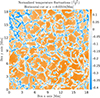 |
Fig. 1. Horizontal cut of the CO5BOLD 3D simulation box below the photosphere of the normalized temperature. Blue shades correspond to downflows while orange shades identify upflows. The snapshot shown here corresponds to a high-resolution simulation of the Sun performed with CO5BOLD (Grid nodes: 534 × 534 × 424). |
3. Mathematical model
3.1. Starting point
As the formalism is developed in a 3D environment associated with a hydrodynamic simulation, the starting point of our model is the well-known Navier-Stokes equations; given the high Reynolds number present in astrophysical flows, viscosity is left out in this instance. Here we reiterate the continuity, momentum, and conservation of energy equations in a Cartesian reference frame:
 (1)
(1)
 (2)
(2)
 (3)
(3)
where ρ is the density, t the time,  the velocity vector, P the pressure,
  the gravitational acceleration vector, T the temperature, s the entropy and finally
  is the radiative heat flux vector.
In the conservation of energy Eq. (3), we note the presence of the radiative heat flux  . Therefore, coupled with the Navier-Stokes equations (Eqs. (1)–(3)), we define an additional expression to express this physical quantity. We decided to use the classical diffusion equation for the radiative transport, which is valid where the mean free path of photons is negligible, as follows:
 (4)
(4)
where 𝒳 stands for the radiative conductivity.
We apply the perturbative approach to the 3D medium, here applying a small Eulerian perturbation directly to the time- and space-dependent Navier-Stokes equations (Eqs. (1)–(3)). We obtain the following system of coupled equations:
 (5)
(5)
 (6)
(6)
 (7)
(7)
 (8)
(8)
where X′ corresponds the Eulerian perturbation of the physical quantity X.
The physical quantities appearing in these equations (Eqs. (5)–(8)) depend on the three spatial coordinates and time. In particular, the coefficients are directly obtained from 3D hydrodynamic simulations. We aim to solve these for the entire star considered and in this 3D environment. It is worth insisting that a major change of paradigm with the current stellar oscillation models can already be observed. We do not restrict ourselves to the horizontal average, which allows us to avoid introducing challenging parameters or unknowns such as the convective flux in the conservation of energy equation (Eq. (7)) or the Reynolds stress in the conservation of momentum equation (Eq. (6)). This automatically means that the most difficult part of turbulence modeling is avoided, namely the closure equation.
A fundamental distinction can also be observed between our formalism and the various existing approaches based on hydrodynamic simulation (Nordlund & Stein 2001; Belkacem et al. 2019; Zhou et al. 2020). First, we aim to solve the system of equations (Eqs. (5)–(8)) for the entire star and we do not limit our approach to the simulation box. This leads to global oscillation modes and frequencies corresponding to the studied star. Second, in our formalism, as mentioned earlier, turbulence and convection are considered as known data. More specifically, the medium in which the waves propagate is an input provided by a previously computed 3D hydrodynamics simulation and we compute the 3D eigenfunctions corresponding to the oscillation modes (the primed quantities in Eqs. (5)–(8)). Our approach enables us to avoid significant difficulties and limitations associated with other existing 3D approaches. As we do not have to search the oscillation modes present in a 3D simulation, we completely avoid the difficult and problematic task of having to distinguish convection from oscillations in a precomputed 3D simulation. Moreover, our formalism allows us to compute global oscillation modes. Therefore, those global modes are not subject to major inaccuracies associated with box modes present in the simulation: excessively large amplitudes of oscillations due to their overly low inertia artificially enhances nonlinear effects and leads to inaccurate frequencies, and so on. Therefore, our formalism enables us to accurately quantify the 3D modal surface effects on frequencies, which is not possible with box modes. We can illustrate this difference between our formalism and the current 3D approaches based on hydrodynamic simulation modes. Without loss of generality, let us take a physical quantity X as follows:
 (9)
(9)
In our model, we want to solve a small perturbation X′ (unknown stellar oscillation) around an equilibrium position, which is given by the hydrodynamic simulation Xconv (considered data, a coefficient of our system of equations). It immediately follows that convection and stellar oscillations are naturally separated in our formalism.
Nevertheless, a solution cannot be found numerically and further development is required to obtain a solvable system. As we are making use of the perturbative approach and wish to isolate an oscillation mode, we assume a small Eulerian perturbation; we can decompose it into a space-related component  (
( ) and a time-related component ei σt, where σ is the oscillation frequency:
 (10)
(10)
While one might be tempted to use spherical coordinates, we ought to comply to the reference frame used in the 3D hydrodynamic simulation, which is 3D Cartesian (see Sect. 2). After the introduction of this decomposition into our system, we take the Fourier transform of this set of equations at the (unknown) oscillation frequency and over a shorter time interval than the total duration of the 3D simulation:
 (11)
(11)
Equation (11) shows an example of this time integration, where we highlight the case where a coefficient B, that is, any physical quantity of a 3D hydrodynamic simulation, is multiplied by a perturbation A′, any unknown to be solved in our model. In combination with our decomposition of the perturbation (Eq. (10)), this time integration turns the coefficient into a time-averaged coefficient  which then allows us, without loss of generality, to use the local time averages of the physical quantities available in our Large Eddy Simulation as coefficients in our stellar oscillation model. This step is essential in our new formalism as it allows us to remove the time dependency of all the variables, unknowns, and coefficients alike, as illustrated in Eq. (11). After some algebra, we obtain the following set of equations for the continuity, momentum, energy, and radiative transport equations. We note that in the remainder of the paper, the time average symbol “
 ” is omitted for the sake of clarity and therefore any coefficients present in the equations are time averaged, unless clearly specified otherwise.
 (12)
(12)
 (13)
(13)
 (14)
(14)
 (15)
(15)
A new stellar oscillation model must be closer to reality and should avoid relying on free parameters by staying in a 3D environment and capturing the nature of turbulence. This could potentially be undermined if the length of the integration time chosen removes those turbulent characteristics. Indeed, as the length of the integration time is increased, we can lose some features of turbulence such as the amplitude of the motion as well as the smallest timescale of the simulation. Due to the nature of the solar flow in its superficial layer (Rayleigh-Bénard convection), with an ill-chosen time of integration, one might even be able to remove convective cells. Figure 2 shows a comparison between a snapshot and several time-averaged intervals performed over 3, 5 and 10 min with CO5BOLD for the case of the Sun. Comparing the normalized internal energy between a snapshot and a three-minute time average, we can clearly see that the differences in terms of turbulence pattern and intensity of the downflows and upflows are almost negligible. A quick look at the scales and the shape of the convective cells allows us to state that, over three minutes, the features of turbulence have been conserved. With a five-minute time average, the turbulent structure is still similar to the snapshot. While the upflows remain at the same amplitude, we note a small decrease in the maximum amplitude of the downflows. Nonetheless, the features of turbulence are also conserved. Theses similarities between the snapshot and time average strengthen the time processing step of our model, given that the turbulence does not drastically evolve over the typical oscillation period of the Sun. We note that taking a time average that is longer than the oscillation period and convective turn-over time does not lead to the complete removal of turbulence, as the largest scales are stable and preserved, meaning that the average medium in which the modes propagate does not tend to zero. However, with longer time averaging intervals, as shown by the ten-minutes average in Fig. 2, the turbulent features are reduced. Indeed, only the largest scales remain and the amplitudes of the downflows have been significantly diminished. Therefore, in our formalism, shorter time averaging intervals of approximately one oscillation period are recommended in order to avoid the loss of some features of turbulence.
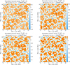 |
Fig. 2. Comparison between a snapshot of the normalized internal energy (top left panel) and time averages over 3 min (top right), 5 min (bottom left), and 10 min (bottom right). Blue shades correspond to downflows while orange shades signal upflows. The snapshots shown here corresponds to low resolution simulations of the Sun performed with CO5BOLD (Grid nodes: 189 × 189 × 150). |
3.2. Fourier approach
Solving the system in its current state (Eqs. (12)–(15)) is still out of reach for most numerical schemes and algorithms. Consequently, we use the Fourier series and transforms to derive the final state of our new formalism. We note that we work with a spatial approach in the Fourier domain. Without loss of generality, one can express the variables of our system of equations, unknown perturbations (e.g., ρ′, T′), and 3D simulation quantities and coefficients (e.g., ρ, 𝒳) alike as a 2D Fourier series in the horizontal plane  :
:
 (16)
(16)
 (17)
(17)
where m,n are summation indexes, Nx is the number of nodes in the x direction, Ny is the number of nodes in the y direction,  , Δx,Δy are the mesh spatial resolutions in the horizontal plane,
  stands for a 3D simulation quantity (coefficient), and
  represents a perturbation (unknown).
Before further presentation of our formalism, it might be useful to briefly discuss the reasons for and relevance of using the spatial Fourier transforms as a tool to solve our system of coupled partial differential equations established in real space (Eqs. (12)–(15)). First, we insist on the fact that the Fourier transforms are only a tool used to resolve the oscillation equations in 3D. Once a solution is found, an inverse Fourier transform is used to return to real space, enabling us to verify that Eqs. (12)–(15) have been precisely solved and to interpret the results. Second, as detailed in Sect. 4, introducing the Fourier series (Eqs. (16) and (17)) allows us to obtain a natural distinction between the horizontal average value and the fluctuations around this horizontal average value. Indeed, looking at a Fourier series of a coefficient of our system of equations,  (Eq. (16)), we can immediately see that the term k = 0 in the sum corresponds to the horizontal average value of A at a given z-coordinate, while the remaining terms (k ≠ 0) represent fluctuations around this horizontal average value. This natural distinction between horizontal average and fluctuations is crucial in order to obtain the desired state of our system of equations and to solve them numerically. This distinction can just as easily be illustrated in real space via Eq. (9). Without loss of generality, Xconv and X′ alike can be decomposed into their horizontal average and fluctuations as follows:
 (18)
(18)
We reexpressed Xconv as Xconv, avg and Xconv, fluc where Xconv, fluc is defined as Xconv − Xconv, avg. After a similar decomposition of the oscillations X′, we obtained Eq. (18). The parallel with the Fourier space is then straightforward. We recall here that this decomposition into horizontal average and fluctuations is performed on both 3D hydrodynamic quantities and perturbations. Whether horizontal average or fluctuation, we note that any quantity coming from the hydrodynamic simulation is considered known and is used as a coefficient in the equations.
Using Fourier series (Eqs. (16) and (17)) to express physical quantities from the simulation is possible due to the periodic boundary conditions used for the four sides of the CO5BOLD box. Regarding the perturbation, the periodicity condition in the horizontal plane is also naturally implied and a Fourier series expansion is then possible. Indeed, assuming a nonzero resulting horizontal perturbation, an aperiodic perturbation in the horizontal plane would result in a global stellar motion in one of the horizontal directions, which is incompatible with the observations. Applying this decomposition in 2D Fourier series (Eqs. (16) and (17)) to our system of equations (Eqs. (12)–(15)) leads to the following in terms of continuity, momentum, energy, and radiative transport:
![Mathematical equation: $$ \begin{aligned}&\sum _{{k}_1} \Big \{i \sigma \,\rho _{{k}_1}^\prime \, \mathrm{e} ^{i \,\underline{k}_1\cdot \underline{x}}\Big \} + \sum _{{k}_1}\sum _{{k}_2} \left\{ [i(\underline{k}_1+\underline{k}_2)] \cdot \rho _{{k}_1}^\prime \, \underline{v}_{{h,k}_2} \,\mathrm{e} ^{i(\underline{k}_1 +\underline{k}_2) \cdot \underline{x}} + [i(\underline{k}_1+\underline{k}_2)] \cdot \rho _{{k}_1}\, \underline{v}_{{h,k}_2}^\prime \, \mathrm{e} ^{i(\underline{k}_1+\underline{k}_2) \cdot \underline{x}} \right\} \nonumber \\&\quad + \sum _{{k}_1}\sum _{{k}_2} \Big \{ \frac{\partial }{\partial z} \left( \rho _{{k}_1}^\prime \, v_{{z,k}_2}\right) \mathrm{e} ^{i(\underline{k}_1+\underline{k}_2)\cdot \underline{x}} + \frac{\partial }{\partial z}\left(\rho _{{k}_1}\, v_{{z,k}_2}^\prime \right) \mathrm{e} ^{i(\underline{k}_1+\underline{k}_2)\cdot \underline{x}} \Big \} = 0, \end{aligned} $$](/articles/aa/full_html/2024/04/aa46346-23/aa46346-23-eq32.gif) (19)
(19)
![Mathematical equation: $$ \begin{aligned}&\sum _{{k}_1}\Big \{ i\sigma \, \underline{v}_{{k}_1}^\prime \, \mathrm{e} ^{i \,\underline{k}_1\cdot \underline{x}}\Big \} +\sum _{{k}_1}\sum _{{k}_2} \Big \{\underline{v}_{{h,k}_1}^\prime \cdot (i\,\underline{k_2}) \otimes \underline{v}_{{k}_2} +\underline{v}_{{h,k}_1} \cdot (i\,\underline{k_2}) \otimes \underline{v}_{{k}_2}^\prime \,\mathrm{e} ^{i(\underline{k}_1+\underline{k}_2) \cdot \underline{x}}\Big \}\nonumber \\&\quad + \sum _{{k}_1}\sum _{{k}_2} \Big \{v_{z,k_1}^\prime \,\frac{\partial }{\partial z}\left(\underline{v}_{{k}_2}\right) \, \mathrm{e} ^{i(\underline{k}_1+\underline{k}_2) \cdot \underline{x}}+v_{z,k_1} \,\frac{\partial }{\partial z}\left(\underline{v}_{{k}_2}^\prime \right) \Big \}= -\sum _{{k}_1}\sum _{{k}_2} \Big \{i\underline{k_1} \, P_{{k}_1}^\prime \, \left(\frac{1}{\rho }\right)_{{k}_2} \, \mathrm{e} ^{i(\underline{k}_1+\underline{k}_2) \cdot \underline{x}} \, + \,i\underline{k_1} \, P_{{k}_1} \, \left(\frac{1}{\rho }\right)_{{k}_2}^\prime \, \mathrm{e} ^{i(\underline{k}_1+\underline{k}_2) \cdot \underline{x}}\nonumber \\&\quad + \underline{e}_{{z}} \left[\frac{\partial P_{{k}_1}^\prime }{\partial z}\,\left(\frac{1}{\rho }\right)_{{k}_2}+\frac{\partial P_{{k}_1} }{\partial z}\,\left(\frac{1}{\rho }\right)_{{k}_2}^\prime \right]\, \mathrm{e} ^{i(\underline{k}_1+\underline{k}_2) \cdot \underline{x}} \Big \} +\sum _{{k}_1} \underline{g}_{{k}_1}\, \mathrm{e} ^{i \,\underline{k}_1\cdot \underline{x}}, \end{aligned} $$](/articles/aa/full_html/2024/04/aa46346-23/aa46346-23-eq33.gif) (20)
(20)
 (21)
(21)
 (22)
(22)
where ⊗ denotes the dyadic product,  is the unit vector in the z/radial direction, and k1 and k2 are arbitrary summation indexes.
In Eqs. (19)–(22), we note several major consequences from the introduction of our 2D Fourier decomposition (Eqs. (16) and (17)). First, any product turns into double summations. Second, any horizontal gradient or divergence is replaced by a product following the well-known properties of the Fourier series or transforms. Third and finally, the only remaining derivatives are with respect to the radial coordinate z, which is hereafter the only independent variable of our system of equations.
After introducing the 2D Fourier decomposition, double summations appeared. To remove this inconvenience, we can project our system of equations (Eqs. (19)–(22)) in a specific direction of the Fourier space (horizontal plane). Let us use  to denote an arbitrary direction in the 2D Fourier space. Projecting any quantity A, an equation in our case, is simply done in the Fourier space by applying the following integral, where Σ stands for the horizontal surface:
 (23)
(23)
Applying this projection (Eq. (23)) to our system of equations (Eqs. (19)–(22)) leads to specific relations between the three parameters  (direction of the projection),
  and
and  (both parameters of the decomposition in 2D Fourier series). Those relations can be established based on the two possibilities that can already be observed in the continuity equation (Eq. (19)). The whole purpose of this projection is to provide a link between our previously independent parameters
  and
and  from the Fourier series decomposition.
The first relation can be derived based on the projection of the first term of the continuity equation. As we apply a surface integral, only the imaginary exponential remains as an integrand, which leads to the following relation in order to avoid a trivial result:
 (24)
(24)
The second relation can be derived similarly based on the projection of the second term of the continuity equation this time. Once again applying the surface integral, only the imaginary exponential remains as an integrand, which leads us to the following relation in order to avoid a trivial result:
 (25)
(25)
Using these two established relations (Eqs. (24) and (25)) derived from the projection in the specific direction  , after some algebra, we can rewrite our system of equations as a convolution product in the Fourier space and obtain the following for the continuity, momentum, energy, and radiative transport (we note that we replaced the summation index k1 with k to simplify the notations):
 (26)
(26)
![Mathematical equation: $$ \begin{aligned}&i\sigma \, \underline{v}_{{k}_0}^\prime + \, \sum _{{k}} \Big \{i\,\underline{v}_{{h,k}}^\prime \cdot (\underline{k_0}-\underline{k}) \otimes \underline{v}_{{k}_0{-k}} +i\,\underline{v}_{{h,k}} \cdot (\underline{k_0}-\underline{k}) \otimes \underline{v}_{{k}_0{-k}}^\prime +v_{{z,k}}^\prime \,\frac{\partial }{\partial z}\left(\underline{v}_{{k}_0{-k}}\right)+v_{{z,k}} \,\frac{\partial }{\partial z}\left(\underline{v}_{{k}_0{-k}}^\prime \right) \Big \} \nonumber \\&{=}~-\sum _{{k}} \Big \{i\underline{k} \, P_{{k}}^\prime \, \left(\frac{1}{\rho }\right)_{{k}_0{-k}} \, + \,i\underline{k} \, P_{{k}} \, \left(\frac{1}{\rho }\right)_{{k}_0{-k}}^\prime + \underline{e}_{{z}} \left[\frac{\partial P_{{k}}^\prime }{\partial z}\,\left(\frac{1}{\rho }\right)_{{k}_0{-k}}+\frac{\partial P_{{k}} }{\partial z}\,\left(\frac{1}{\rho }\right)_{{k}_0{-k}}^\prime \right] \Big \}\, +\, \underline{g}_{{k}_0}^\prime , \end{aligned} $$](/articles/aa/full_html/2024/04/aa46346-23/aa46346-23-eq48.gif) (27)
(27)
 (28)
(28)
 (29)
(29)
The advantages of this 2D Fourier decomposition and then projection are as follows. First and foremost, the 2D Fourier space turns a system of coupled partial differential equations into a system of differential equations with only one independent variable, the radial coordinate z, for each value of k0 (we note that k and k0 are evaluated at the nodes of the simulation box). Once its value is set, the algebraic form of our system of equations is now in an ideal state to be solved by many different numerical schemes. Presently, a large quantity of unknowns or data are no longer considered an inconvenience with the capabilities of modern computers, which are able to store massive amounts of data and carry out efficient parallelization. However, reaching a simpler version of an equation can be a key factor in the stability and efficiency of the numerical solver. Second, we obtained a natural distinction between the horizontal average equations (comparable to the 1D model currently in use) when the value of k0 is set to zero in our system of equations, and the different scales of turbulence, any value of k0 different from 0. Hence, our model allows us to assess the impact of all the different scales of the turbulent spectrum on the stellar oscillations and ultimately their individual contributions to the eigenfrequencies and damping rates of the modes. Finally, being in Fourier space does not induce any drawbacks to our model, because once a solution is found, we can easily access the real space by a simple inverse Fourier transform.
4. Scales of our formalism
We now discern the horizontal average (k0 = 0) from fluctuation (k0 ≠ 0) equations and derive the final form of our new global nonadiabatic oscillation equations in a full 3D framework. While our formalism sets the mathematical foundation of a new 3D stellar oscillation model, it has to be borne in mind that a solution to this system of equations is only achievable via the use of a numerical scheme and an iterative method. Although a specific numerical scheme to solve the problem is out of the scope of this paper and will be presented in a subsequent paper of this series, it is nevertheless implied that, during the iterative process, a decoupling will be performed between the average unknowns and the many fluctuations (see Sect. 5). In the hydrodynamic simulation, the average (k = 0) of physical quantities is larger than their fluctuations (k ≠ 0), with the exception of the velocities. In Figs. 1 (temperature) and 2 (internal energy), we can clearly observe that the fluctuations are indeed small in comparison to the horizontal average values, being around 10%–20% of the horizontal average values for the most part and very locally up to 40%. Hence, we assume that this trend will be followed by the 3D eigenfunctions. This hypothesis will have to be verified a posteriori and, in the first instance, leads us to first limit our approach to quasi-radial modes and, later, to nonradial modes of low l degrees. Consequently, a small change of any fluctuation is not expected to lead to a significant modification of the Fourier series, which is dominated by the average term. Therefore, in the following sections when dealing with the average equations, it is assumed that the fluctuations (unknowns for each k ≠ 0) were determined in a previous step of the algorithm and are then fixed when average equations are to be solved. The same assumption is applied when fluctuation equations are considered, although in that case the average unknowns (k = 0) are fixed and assumed solved in a previous step. We note that, although the fluctuation oscillations are small, they impact the average oscillations, and their contribution as a whole has a dominant effect on the damping and therefore on the modal contribution to the surface effects. Indeed, these fluctuation oscillations constitute, amongst other things, the perturbation of the turbulent pressure, which is known to be a major contribution to the damping of the modes in solar-like oscillations (Houdek & Dupret 2015; Samadi et al. 2015).
4.1. Average equations k0 = 0
The equations for the horizontal average perturbations correspond to k0 = 0 in the general form of our system (Eqs. (26)–(29)). After some algebra, we get the following for the horizontal average perturbations:
 (30)
(30)
 (31)
(31)
 (32)
(32)
 (33)
(33)
 (34)
(34)
 (35)
(35)
As we are working with real data from the 3D hydrodynamic simulation, A−k is simply – according to the properties of Fourier transform – the complex conjugate of Ak (noted  ). Here, we note that we have separated the equations of momentum conservation (Eqs. (31) and (32)) as well as those of radiative transport (Eqs. (34) and (35)) into a radial and a horizontal component. Following a direct investigation of the horizontal radiative flux
  in this system of equations, we can immediately note that this latter only appears in Eq. (35) and is fully determined by the fluctuations, because the first term of the sum (k = 0) is trivial. Regarding the horizontal velocity
  , a closer examination of the system leads to the conclusion that this unknown is decoupled from the remaining horizontal average equations. Indeed, the horizontal average velocity only appears in its own equation (Eq. (32)) and is fully determined by the average radial velocity and the fluctuations, as shown in the following, where fluctuations are gathered in one variable
  :
:
 (36)
(36)
Therefore, this equation can be solved in a later step once the radial velocity has been solved or even ignored if the perturbation of the horizontal velocity is not important for a specific use of this formalism.
When dealing with the average equations of our Fourier expansion of the perturbed Navier-Stokes equations, as shown above, two of the six equations can be decoupled from the four remaining ones. However, in those four remaining equations, we highlight the presence of more unknowns than equations even when fixing the values of all the fluctuations. However, those unknowns are not totally independent and can be reexpressed via an equation of state. For this work, we use the pressure  , entropy
  , radial velocity
  , and the radial radiative flux
  as independent variables. Every other unknown perturbation is then expressed via an equation of state in terms of pressure and entropy. Appendix A provides an explanation of how each equation of state was obtained. Here, we only reiterate the general form of the equation of state used in the case k0 = 0 (average perturbations):
 (37)
(37)
where Xeosk regroups all the fluctuations as detailed in Appendix A.
We also restate here that, in the following developments, we consider any order k (k ≠ 0) unknown fluctuation of our problem to be fixed and determined in the previous step of the numerical scheme. Therefore, we regroup all those terms under one variable as demonstrated in the horizontal velocity equation (Eq. (36)) or in the following continuity equation (see Sect. 4.1.1). To obtain an eigenvalue problem, we introduce the following decomposition of the eigenfrequency σ:
 (38)
(38)
where σ0 is the initial eigenfrequency guess and δσ corresponds to the correction.
With this decomposition, the system of equations takes the canonical form of an eigenvalue problem:
 (39)
(39)
Under this form (Eq. (39)), the global eigenvalue problem can be solved by various numerical algorithms, such as the inverse iteration algorithm, to compute the eigenvectors. This algorithm and the decomposition of the eigenvalue are commonly used in nonadiabatic codes for stellar oscillations, where the adiabatic eigenvalue is typically taken as the initial guess. As the surface effects are small (Christensen-Dalsgaard et al. 1996; Houdek & Dupret 2015; Samadi et al. 2015), δσ is much smaller than σ0 and the numerical convergence is fast. Let us now take a closer look at each equation describing the average perturbations in order to derive their final form in our formalism.
4.1.1. Average continuity equation
From the general form of the average continuity equation (Eq. (30)), we can split the summation and separate the first term (k = 0) from all the remaining terms (k ≠ 0). By doing so, we can regroup all the fluctuations under one variable C0bk and simplify the form of the equation as:
 (40)
(40)
Using the equations of state for reexpressing the density from Appendix A and our decomposition of σ (Eqs. (38)), we obtain the final form of the average continuity equation:
![Mathematical equation: $$ \begin{aligned}&C_{{0\mathrm{d}P}}\,\frac{\partial P_{0}^\prime }{\partial z}+C_{{0P}}\,P_{0}^\prime +C_{{0\mathrm{d}s}}\,\frac{\partial s_{0}^\prime }{\partial z}+C_{{0s}}\,s_{0}^\prime +C_{{0\mathrm{d}vz}}\,\frac{\partial v_{{z,0}}^\prime }{\partial z}+C_{{0vz}}\,v_{{z,0}}^\prime +C_{0}=\delta \sigma \,\left[-i\,\rho _{{P}_0}\,P_0^\prime - i\,\rho _{{s}_0}\,s_0^\prime \,-i\,\rho _{{eosk}}\right]. \end{aligned} $$](/articles/aa/full_html/2024/04/aa46346-23/aa46346-23-eq70.gif) (41)
(41)
4.1.2. Average radial momentum equation
From the radial component of the momentum equation (Eq. (31)), we immediately have
 (42)
(42)
In this expression (Eq. (42)), the Eulerian perturbation of a body force, the gravity  , appears. Unlike state variables, where we have a set of equations with which to substitute them in terms of our independent variables, a body force cannot be expressed in such a manner. Nonetheless, an expression for the gravity is available:
 (43)
(43)
For this specific case, a Lagrangian perturbation will be implied instead of the Eulerian one used so far. Indeed the Lagrangian perturbation is more convenient when dealing with the mass, because we are in the superficial layer of the star, and the mass in the gravity expression can be approximated by the total mass of the star, whose envelope has a negligible mass. Consequently, the Lagrangian perturbation of the mass is trivial and the Eulerian perturbation of the gravity can be recovered via the well-known Euler–Lagrange relation. After some algebra, an expression for the perturbation of gravity is derived as follows:
 (44)
(44)
Using Eq. (44) in combination with the equation of state for the specific volume (see Appendix A) and our decomposition of σ (Eq. (38)) in Eq. (42), the radial component of the momentum reads as
![Mathematical equation: $$ \begin{aligned}&M_{{z0\mathrm{d}vz}}\,\frac{\partial v_{{z,0}}^\prime }{\partial z}+M_{{z0vz}}\,v_{{z,0}}^\prime +M_{{z0\mathrm{d}P}}\,\frac{\partial P_{0}^\prime }{\partial z}+M_{{z0P}}\,P_{0}^\prime +M_{{z0s}}\,s_{0}^\prime +M_{{z0}}=\delta \sigma \,\left[(-i+\sigma _0^{-2}\,M_{{0g}})\, v_{{z,0}}^\prime \right]. \end{aligned} $$](/articles/aa/full_html/2024/04/aa46346-23/aa46346-23-eq75.gif) (45)
(45)
4.1.3. Average horizontal momentum equation
As already demonstrated in the beginning of this section, the horizontal component of the momentum equation (Eq. (36)) is decoupled from our system of equations and can be solved once the radial velocity is computed. Nevertheless, we reexpress it in a similar form to the remaining equations. Our decomposition of σ, as in Eq. (38), leads, after some algebra, to
![Mathematical equation: $$ \begin{aligned} M_{{h0\mathrm{d}vh}}\,\frac{\partial }{\partial z}\left(\underline{v}_{{h,0}}^\prime \right)+M_{{h0vh}}\,\underline{v}_{{h,0}}^\prime +\underline{M}_{{h0vz}}\,v_{{z,0}}^\prime +\underline{M}_{{h0k}}=\delta \sigma \,\left[-i\,\underline{v}_{{h,0}}^\prime \right]. \end{aligned} $$](/articles/aa/full_html/2024/04/aa46346-23/aa46346-23-eq76.gif) (46)
(46)
4.1.4. Average radial radiative flux equation
Given that the horizontal component of the radiative flux is entirely determined by the fluctuations (Eq. (35)), no further developments are required. However, this is not the case for the radial component of the radiative flux (Eq. (34)), which can be written under the following form:
 (47)
(47)
In this expression, we still need to express  and
and  in terms of our chosen set of independent variables via the use of equations of state (see Appendix A). After some algebra, Eq. (34) becomes
 (48)
(48)
4.1.5. Average energy equation
Based on the energy equation (Eq. (33)) and grouping all the fluctuation (k ≠ 0) terms, we have
 (49)
(49)
We resort to equations of state (see Appendix A) to obtain an equation expressed solely in terms of our independent variables. So far, we have kept the material derivative of the entropy in our system of equations. However, a material derivative is not compatible with a numerical scheme, because all other derivatives are partial ones. To substitute this term in the energy equation (Eq. (49)), we use the expression (Eq. (B.3)) developed in Appendix B. Finally, applying our decomposition of σ (Eq. (38)) leads to
![Mathematical equation: $$ \begin{aligned}&E_{{0\mathrm{d}s}}\,\frac{\partial s_{0}^\prime }{\partial z}+E_{{0s}}\,s_{0}^\prime +E_{{0P}}\,P_{0}^\prime +E_{{0\mathrm{d}vz}}\,\frac{\partial v_{{z,0}}^\prime }{\partial z} +\frac{\partial }{\partial z}\left(F_{{z,0}}^\prime \right)+E_{0} =\delta \sigma \,\left[-i\,\left(\rho T\right)_0^*\,s_0^\prime \right]. \end{aligned} $$](/articles/aa/full_html/2024/04/aa46346-23/aa46346-23-eq82.gif) (50)
(50)
4.2. Fluctuation equations k0 ≠ 0
We have now established the final form of the average equations of our Fourier expansion of the perturbed Navier-Stokes equations. The second part of the problem consists in describing the fluctuation equations following our formalism in the 2D Fourier space (Eqs. (26)–(29)). For each fluctuation, we have an associated value of k0 leading to a system of equations to solve for this peculiar fluctuation. Moreover, due to the convolution products, each fluctuation is coupled to the average term and all the other fluctuations. Trying to solve such a system of equations would simply be too costly in terms of computation time in the current form of the fluctuation equations. With a full coupling between the scales, this corresponds to the perturbed full 3D Navier-Stokes equations expressed in the Fourier space. Therefore, in order to obtain a solvable system, we have to make some simplifying assumptions.
In Sect. 4, we stated an important hypothesis according to which the average term of the Fourier series dominates the others. Based on this assumption, we split our system into average and fluctuation equations. In the fluctuation equations, this assumption,  , leads to a simplification of the convolution product in our system of equations (Eqs. (26)–(29)). This is also related to the real space where the average quantities are much larger than the fluctuations. In consequence, for each fluctuation equation (k0 fixed) in each convolution product, all terms are neglected, except for the dominating one corresponding to the coupling between a fluctuation and an average value. With this working hypothesis, two important observations can be made. On the one hand, we decouple each fluctuation (except through the average values) and, on the other hand, we have reached a state for our system of equations where parallel algorithms can be used to obtain a numerical solution. Following our working hypothesis, we can derive a system of equations for each fluctuation where, as in the average equations, the momentum equation and radiative transport have been split into a radial and a horizontal component.
 (51)
(51)
![Mathematical equation: $$ \begin{aligned}&i\sigma \,v_{{z,k}}^\prime +\frac{\partial }{\partial z}\left(v_{{z,0}}^\prime \,v_{{z,k}}+v_{{z,0}}\,v_{{z,k}}^\prime \right)+i\,\underline{v}_{{h,0}}^\prime \cdot \underline{k}\,v_{{z,k}}+i \underline{v}_{{h,0}}\cdot \underline{k}\,v_{{z,k}}^\prime =-\left[\frac{\partial P_0^\prime }{\partial z}\,\left(\frac{1}{\rho }\right)_{{k}} + \frac{\partial P_0 }{\partial z}\,\left(\frac{1}{\rho }\right)_{{k}}^\prime +\frac{\partial P_{{k}}^\prime }{\partial z}\,\left(\frac{1}{\rho }\right)_{0}+\frac{\partial P_{{k}} }{\partial z}\,\left(\frac{1}{\rho }\right)_{0}^\prime \right], \end{aligned} $$](/articles/aa/full_html/2024/04/aa46346-23/aa46346-23-eq85.gif) (52)
(52)
![Mathematical equation: $$ \begin{aligned}&i\sigma \, \underline{v}_{{h,k}}^\prime \, +\,v_{{z,0}}^\prime \,\frac{\partial }{\partial z}\left(\underline{v}_{{h,k}}\right)+v_{{z,0}} \,\frac{\partial }{\partial z}\left(\underline{v}_{{h,k}}^\prime \right) +v_{{z,k}}^\prime \,\frac{\partial }{\partial z}\left(\underline{v}_{{h,0}}\right)+v_{{z,k}} \,\frac{\partial }{\partial z}\left(\underline{v}_{{h,0}}^\prime \right) + i\,\underline{v}_{{h,0}}^\prime \cdot \underline{k} \otimes \underline{v}_{{h,k}} + \underline{v}_{{h,0}} \cdot \underline{k} \otimes \underline{v}_{{h,k}}^\prime = -i\underline{k} \,\left[ P_{{k}}^\prime \, \left(\frac{1}{\rho }\right)_{0} + P_{{k}} \, \left(\frac{1}{\rho }\right)_{0}^\prime \right], \end{aligned} $$](/articles/aa/full_html/2024/04/aa46346-23/aa46346-23-eq86.gif) (53)
(53)
 (54)
(54)
![Mathematical equation: $$ \begin{aligned}&F_{{z,k}}^\prime =-\left[\mathcal{X} _0^\prime \,\frac{\partial }{\partial z}\left(T_{{k}}\right)+\mathcal{X} _{0}\,\frac{\partial }{\partial z}\left(T_{{k}}^\prime \right)+\mathcal{X} _{{k}}^\prime \,\frac{\partial }{\partial z}\left(T_{0}\right)+\mathcal{X} _{{k}}\,\frac{\partial }{\partial z}\left(T_{0}^\prime \right)\right], \end{aligned} $$](/articles/aa/full_html/2024/04/aa46346-23/aa46346-23-eq88.gif) (55)
(55)
![Mathematical equation: $$ \begin{aligned}&\underline{F}_{{h,k}}^\prime =-i\left[\mathcal{X} _0^\prime \,\left(\underline{k}\right)T_{{k}}+\mathcal{X} _{0}\,\left(\underline{k}\right)T_{{k}}^\prime \right]. \end{aligned} $$](/articles/aa/full_html/2024/04/aa46346-23/aa46346-23-eq89.gif) (56)
(56)
We note that the index of the fluctuation is now denoted by k and no longer k0 in order to avoid confusion and to simplify the notation, because a given fluctuation is only coupled with the average (index 0) from now on.
While there is only one set of equations for the average perturbations in every scenario possible, depending on the grid resolution of the hydrodynamic simulation, the number of turbulent scales can increase significantly. If we assume a 3D simulation box with N by M nodes in the horizontal plane, applying the 2D Fourier transform would lead to N × M fluctuations and consequently the same number of equations in the system to be solved. A robust example is provided by the case of the low-resolution CO5BOLD simulation shown in Fig. 2, which involves 35 721 different fluctuations, compared to the high-resolution simulation in Fig. 1, which implies 264 196. With such an important and rapidly increasing number of fluctuations to be solved, reducing the number of equations describing a fluctuation can lead to a drastic reduction in computation time and improvement of the parallelization of our formalism.
We propose a substitution of the equations of momentum (Eqs. (52) and (53)) in the continuity equation (Eq. (51)), as well as a substitution of the radiative flux (Eqs. (55) and (56)) in the conservation of energy equation (Eq. (54)), giving rise to, respectively, the continuity-momentum and energy–radiation equations (see Sects. 4.2.1 and 4.2.2). Similarly to the average equations, at this point, we still have more unknowns than equations and some unknowns will be reexpressed via an equation of state, whose general form, when fluctuations are considered, is
 (57)
(57)
For more details regarding the equations of state and there developments, please refer to Appendix A. When dealing with the equations for the fluctuations of our Fourier expansion of the perturbed Navier-Stokes equations, we keep the pressure  and entropy
  as independent variables. In the following developments, as mentioned in Sect. 3.2, we consider that any average unknown or perturbation of our problem is fixed and was determined in the previous step when we solved for the average equations. Therefore, we regroup all those under one variable.
4.2.1. Continuity–momentum equation
To obtain the continuity–momentum equation, we start from the continuity equation (Eq. (51)), which is multiplied by iσ, and where all known terms, average and simulation data, are regrouped in Ck0. After some algebra, we have
 (58)
(58)
Regarding the radial component of the momentum equation (Eq. (52)), we assume the average radial velocity vz, 0 to be small due to a compensation between the upflows and downflows, which automatically leads to  . Moreover, in the simulation box, with periodic boundary conditions and the type of turbulent flows in the superficial layers of stars (Rayleigh-Bénard convection), there is no physical reasons for a resulting average horizontal motion (
 ). From this observation, it is safe to assume that
  . Based on those observations and hypotheses, alongside injecting equations of state (see Appendix A), the following expression for the radial velocity fluctuation can be derived:
![Mathematical equation: $$ \begin{aligned}&i\sigma \,\underline{v}_{{z,k}}^\prime +\frac{\partial }{\partial z}\left(v_{{z,0}}^\prime \,v_{{z,k}}\right)+i\,v_{{z,k}}\,\left(\underline{v}_{{h,0}}^\prime \cdot \underline{k}\right)=-\left[\frac{\partial P_0^{\prime } }{\partial z}\,\left(\frac{1}{\rho }\right)_{{k}}\,+\frac{\partial P_0 }{\partial z}\,\left(\frac{1}{\rho }\right)_{{k}}^\prime +\frac{\partial P_{{k}}^\prime }{\partial z}\,\left(\frac{1}{\rho }\right)_{0}+\frac{\partial P_{{k}} }{\partial z}\,\left(\frac{1}{\rho }\right)_{0}^\prime \right], \end{aligned} $$](/articles/aa/full_html/2024/04/aa46346-23/aa46346-23-eq97.gif) (59)
(59)
 (60)
(60)
As for the horizontal momentum equation (Eq. (53)), similar hypotheses can be made regarding vz, 0 and  , which means that the following terms can be neglected:
  ,
, and
and  . Finally, for the horizontal component of the momentum equation, we obtain
![Mathematical equation: $$ \begin{aligned}&i\sigma \, \underline{v}_{{h,k}}^\prime + v_{{z,0}}^\prime \,\frac{\partial }{\partial z}\left(\underline{v}_{{h,k}}\right)+v_{{z,k}} \,\frac{\partial }{\partial z}\left(\underline{v}_{{h,0}}^\prime \right)+ i\,\underline{v}_{{h,0}}^\prime \cdot \underline{k} \otimes \underline{v}_{{h,k}} = -i\underline{k} \,\left[ P_{{k}}^\prime \, \left(\frac{1}{\rho }\right)_{0} + P_{{k}} \, \left(\frac{1}{\rho }\right)_{0}^\prime \right], \end{aligned} $$](/articles/aa/full_html/2024/04/aa46346-23/aa46346-23-eq103.gif) (61)
(61)
 (62)
(62)
It is worth noting that the equation for the horizontal momentum was kept in order to remain as complete as possible. However, the question of its relevance in our model, whether quantitative or qualitative, remains open and will most likely be answered once a numerical solution is found. With the new expression derived for the horizontal (Eq. (62)) and radial velocities (Eq. (60)), we can substitute  ,
,  as well as
  via the equation of state (see Appendix A) into the continuity equation (Eq. (58)), which leads to the following:
 (63)
(63)
Finally, introducing our decomposition of σ as in Eq. (38) and injecting it into the previous equation (Eq. (63)) leads, after some algebra, to the continuity–momentum equation, a second-order linear differential equation:
![Mathematical equation: $$ \begin{aligned}&\mathrm{CM}_{k\mathrm{dd}P}\frac{\partial ^2 P_{k}^\prime }{\partial z^2} + \mathrm{CM}_{k\mathrm{d}P}\frac{\partial P_{k}^\prime }{\partial z} + \mathrm{CM}_{kP}P_{k}^\prime + \mathrm{CM}_{k\mathrm{d}s}\frac{\partial s_{k}^\prime }{\partial z} + \mathrm{CM}_{ks}s_{k}^\prime + \mathrm{CM}_{kb0}\nonumber \\&= \delta \sigma \,\left[\mathrm{CM}_{{k\mathrm{d}}\sigma {P}} P_{{k}}^\prime +\mathrm{CM}_{{k\mathrm{d}}\sigma {\mathrm{d}P}} \frac{\partial P_{{k}}^\prime }{\partial z}+\mathrm{CM}_{{k\mathrm{d}}\sigma {s}} s_{{k}}^\prime +\mathrm{CM}_{{k\mathrm{d}}\sigma {\mathrm{d}s}} \frac{\partial s_{{k}}^\prime }{\partial z}+\mathrm{CM}_{{k\mathrm{d}}\sigma {0}}\right]. \end{aligned} $$](/articles/aa/full_html/2024/04/aa46346-23/aa46346-23-eq109.gif) (64)
(64)
4.2.2. Energy–radiation equation
To derive the energy–radiation equation, we begin with the energy equation (Eq. (54)) multiplied by iσ and where all known terms have been grouped under one variable Ek0. We immediately obtain:
 (65)
(65)
In the left-hand side of the energy equation (Eq. (65)), we have the material derivative of the entropy (see Eq. (B.4)); multiplying it by iσ, substituting the movement equation for  (Eq. (60)), and carrying out some algebra, we obtain
![Mathematical equation: $$ \begin{aligned}&i\sigma \,\left(\frac{\mathrm{D}s}{\mathrm{D}t}\right)_{k}^\prime = -\sigma ^2 s_{k}^\prime + i\sigma \,v_{{z,0}}\,\frac{\partial }{\partial z}\left(s_{k}^\prime \right) - \sigma \,\underline{v}_{{h,0}}\cdot \underline{k}\,s_{k}^\prime + i\sigma \,\mathrm{SB} + \frac{\partial }{\partial z}\left(s_0\right)\left[M_{zkb0} + M_{zkP}P_{k}^\prime + M_{zks}s_{k}^\prime + M_{zk\mathrm{d}P}\frac{\partial P_{k}^\prime }{\partial z}\right], \end{aligned} $$](/articles/aa/full_html/2024/04/aa46346-23/aa46346-23-eq112.gif) (66)
(66)
where SB regroup all the average perturbations as defined in Eq. (B.4).
Now we focus our interest on the right-hand side of Eq. (65). Multiplying the radiation equations for the radial (Eq. (55)) and horizontal (Eq. (56)) fluxes (Fz, k′ and  ) by iσ and substituting the equations of state for Tk′ and 𝒳k′ (see Appendix A), we obtain
![Mathematical equation: $$ \begin{aligned}&i\sigma \,F_{z,k}^\prime = i\sigma \left[-R_{zk\mathrm{d}P}\,\frac{\partial P_{k}^\prime }{\partial z} - R_{zk\mathrm{d}s}\,\frac{\partial s_{k}^\prime }{\partial z} - R_{zkP}\,P_{k}^\prime - R_{zks}\,s_{k}^\prime - R_{zkb0}\right], \end{aligned} $$](/articles/aa/full_html/2024/04/aa46346-23/aa46346-23-eq114.gif) (67)
(67)
 (68)
(68)
We can then substitute the material derivative of the entropy  (Eq. (66)), the radial flux
  (Eq. (67)), and the horizontal flux
  (Eq. (68)) in the energy equation (Eq. (65)). With the reexpression of
  in terms of our independent variables via an equation of state (see Appendix A), we derive
![Mathematical equation: $$ \begin{aligned}&-\sigma ^2\,(\rho T)_0\,s_{k}^\prime + \sigma \,\mathrm{ER}_{\sigma {ks}}\,s_{k}^\prime + \sigma \,\mathrm{ER}_{\sigma {kds}}\,\frac{\partial s_{{k}}^\prime }{\partial z}+\sigma \,\mathrm{ER}_{\sigma {kdds}}\,\frac{\partial ^2 s_{{k}}^\prime }{\partial z^2} +\sigma \,\mathrm{ER}_{\sigma {kP}}\,P_{{k}}^\prime +\sigma \,\mathrm{ER}_{\sigma {kdP}}\,\frac{\partial P_{{k}}^\prime }{\partial z}+\sigma \,\mathrm{ER}_{\sigma {kddP}}\,\frac{\partial ^2 P_{k}^\prime }{\partial z^2} + \sigma \,\mathrm{ER}_{\sigma k0} \nonumber \\&\quad +\left(\rho T\right)_{0}\,\frac{\partial }{\partial z}\left(s_0\right)\left[M_{zkb0}+M_{zkP}P_{k}^\prime +M_{zks}s_{k}^\prime + M_{zkdP} \frac{\partial P_{k}^\prime }{\partial z}\right] = 0. \end{aligned} $$](/articles/aa/full_html/2024/04/aa46346-23/aa46346-23-eq120.gif) (69)
(69)
Finally, we introduce our decomposition of σ as in Eq. (38) into the latter expression (Eq. (69)), establishing the energy–radiation equation, which describes the energetic aspects of the fluctuations. Here, we again deal with a second-order linear differential equation as in the continuity–momentum equation (Eq. (64)):
![Mathematical equation: $$ \begin{aligned}&\mathrm{ER}_{{k\mathrm{dd}P}}\frac{\partial ^2 P_{k}^\prime }{\partial z^2} + \mathrm{ER}_{{k\mathrm{d}P}} \frac{\partial P_{k}^\prime }{\partial z} + \mathrm{ER}_{{kP}}P_{k}^\prime +\mathrm{ER}_{k\mathrm{dd}s}\frac{\partial ^2 s_{k}^\prime }{\partial z^2} + \mathrm{ER}_{k\mathrm{d}s}\frac{\partial s_{{k}}^\prime }{\partial z}+\mathrm{ER}_{{ks}}s_{{k}}^\prime +\mathrm{ER}_{{kb0}} = \delta \sigma \,\left[\mathrm{ER}_{{k\mathrm{d}}\sigma {P}} P_{{k}}^\prime +\mathrm{ER}_{{k\mathrm{d}}\sigma {\mathrm{d}P}} \frac{\partial P_{{k}}^\prime }{\partial z}\right.\nonumber \\&\quad \left.+~\mathrm{ER}_{{k\mathrm{d}}\sigma {\mathrm{dd}P}} \frac{\partial ^2 P_{{k}}^\prime }{\partial z^2}+\mathrm{ER}_{{k\mathrm{d}}\sigma {s}} s_{{k}}^\prime +\mathrm{ER}_{{k\mathrm{d}}\sigma {\mathrm{d}s}} \frac{\partial s_{{k}}^\prime }{\partial z}+\mathrm{ER}_{{k\mathrm{d}}\sigma {\mathrm{dd}s}} \frac{\partial ^2 s_{{k}}^\prime }{\partial z^2}+\mathrm{ER}_{{k\mathrm{d}}\sigma {0}}\right]. \end{aligned} $$](/articles/aa/full_html/2024/04/aa46346-23/aa46346-23-eq121.gif) (70)
(70)
5. Eigenvalue problem and extension outside the simulation box
Above, we detail the derivation of our new formalism and set the foundation of an innovative nonadiabatic oscillation code in a full 3D framework. We started from the perturbation of the Navier-Stokes equations, went into the Fourier space, and finally derived a system of equations to characterize the average and fluctuation perturbations in a 3D environment. In a general manner, we can represent these systems of equations with linear operators. The equations describing the average perturbations (Eqs. (41), (45), (48) and (50)) can be grouped and represented by one linear system:
 (71)
(71)
where ℒ0 and ℒ1 correspond to linear operators.
Moreover, each system of equations (Eqs. (64) and (70)) describes a specific fluctuation and corresponds to a given value of k, and can also be put into a linear system form:
 (72)
(72)
where ℒk and ℒf correspond to linear operators.
With these linear systems, we clearly see the appearance of the well-known form of an eigenvalue problem that ends the mathematical developments present in this paper as the desired state of our system of equations has been derived.
While outside the scope of this paper, we can comment on the topic of boundary conditions for our formalism. In Sect. 3, we make use of the optically thick approximation to express the radiative flux (Eq. (4)). However, the hydrodynamic simulation spans beyond the photosphere (see Sect. 2) where the latter is no longer valid. A simple model of nonadiabatic oscillation in that optically thin region was proposed by Dupret et al. (2002). This latter assumes that, because of the very short thermal timescales in the superficial layers, the T(τ) law – with τ being the optical depth – is maintained during the oscillations. This leads us to more closely examine the T − τ relations along different gas columns of a 3D simulation. In Fig. 3, local temperature profiles are shown as a function of the optical depth. While close to the photosphere, the profile seems similar, yet, as we venture into the atmosphere, all the profiles diverge and a simple law T(τ) does not emerge as a reliable solution. Hence, this simple approach does not seem justified for the energetic fluctuation equation and, here, we therefore do not propose a 3D time-dependent convection model above the photosphere for the fluctuation equations (Eq. (72)). Moreover, this decision is also based on the complexity of the radiative transfer as well as on the low impact (although not negligible) of that region of the star in terms of surface effect and damping of the modes. Indeed, while approximate, the current TDC models indicate that the main contribution to the mode damping in solar-like modes originates from regions below the photosphere with the major contribution coming from the turbulent pressure oscillations; see Balmforth (1992), Houdek & Dupret (2015). We note that the average equations (Eq. (71)) can be extended beyond the photosphere by using the T(τ) law as shown in Dupret et al. (2002).
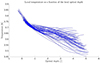 |
Fig. 3. Evolution of the local temperature as a function of the local optical depth in CO5BOLD 3D simulation box. Each curve represents the evolution along one radial column. The data shown here were extracted from a low resolution simulation of the Sun performed with CO5BOLD (Grid nodes: 189 × 189 × 150). |
In this formalism, we want to solve the quasi-radial global nonadiabatic oscillation equations in a full 3D framework, which would provide a description of the stellar oscillation from the center of a star to its photosphere or part of its atmosphere. This “global” term implies that we find how to connect the simulation – which does not represent the entire star – to the remaining part of the stellar structure. For solar-like stars, the 3D simulation box of CO5BOLD (see Sect. 2) is only able to describe the superficial layer of the star. As far as the study of stellar turbulence is concerned, this limitation can easily be understood, because in deeper layers of solar-like stars the medium is stable against convection based on the Schwarzschild criterion and the energy is transported by radiation. Even though the simulation box does not go deep enough into the star to reach the tachocline, the simulation is able to reach regions in a quasi-adiabatic state and to model deeper regions in the convective zone where the entropy reaches a plateau. Figure 4 shows the radial evolution of local entropy in the simulation box. Towards the bottom of the box, we clearly see the local entropy converging toward the average entropy and both reaching a plateau. We note the complex entropy profile in the heart of the convective zone, which emphasizes our remarks made in Sect. 2 regarding the advantages of staying in a 3D environment to capture the nature of turbulence. Indeed, the asymmetry shown on Fig. 1 between the downflows and upflows is also present in the entropy profile. While the upflows have a tendency to remain at the entropy plateau, the downflows have a very wide range of entropy.
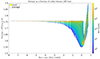 |
Fig. 4. Evolution of the entropy along the radial direction in the CO5BOLD 3D simulation box. The color grading represents the local entropy, while the red curve corresponds to the horizontal average entropy. The entropy shown here was extracted from a low-resolution simulation of the Sun performed with CO5BOLD (Grid nodes: 189 × 189 × 150). |
As the bottom of the simulation is in a quasi-adiabatic state and as deeper in the star the radiative zone is reached (well below the simulation box), we propose to set the fluctuations  to 0 and describe the oscillations solely by the average perturbations in our formalism with the linear system
  derived from our system of equations (see Eq. (71)). In other words, below the simulation box, we propose to come back to a 1D model along the radial direction. This 1D model is coupled with the 3D model used in the 3D box and will affect the average perturbations
  of that region. To ensure a smooth transition from the internal 1D structure to the 3D one, we use a so-called patched model as reference, which ensures the continuity of the average quantities at the bottom of the 3D box. This approach is fully compatible with our formalism, as we stated (see Sect. 3.2) that the average perturbations are solved separately from the fluctuations in the numerical scheme. Therefore, the average perturbation will span the entire star, while the fluctuation will be limited to the radial distance of the simulation box.
6. Work integral and damping of the modes
Now armed with a 3D quasi-radial global nonadiabatic oscillation model, assuming a solution has been computed for each fluctuation as well as the average of all of them (see Sects. 4.1 and 4.2), we can extend the discussion to the post-processing and derive the work integral as well as the expression for the damping rate in our formalism. Indeed, those quantities are not trivial, as perturbations are now expressed in three dimensions and possess specific characteristics linked to the hydrodynamic simulation and assumptions. Unlike Sect. 3.1, we propose to use the equation of momentum under the conservative form, as follows:
 (73)
(73)
where we use the Einstein summation convention in the latter to simplify the notation.
In Eq. (73), the term Rij, which is similar to the Reynolds stress but without averaging, appears naturally. The presence of this term, which we refer to as the Reynolds tensor from now on, is interesting as its impact on the oscillations, and therefore on the damping of the mode, remains an open question in stellar pulsation physics, while its importance has already been stated (e.g., Houdek & Dupret 2015; Belkacem et al. 2021). Following the same steps described in our formalism, the time averaging and an Eulerian perturbation are applied to Eq. (73), which leads to
 (74)
(74)
where  .
.
In order to obtain an expression for energy and then the work, we multiply Eq. (74) by the conjugate of the perturbed velocity  and then integrate over the entire volume of the star, obtaining
 (75)
(75)
On the right-hand side of Eq. (75), we have the contribution to the work integral of the Reynolds tensor, the gas pressure, and the gravity. Regarding the gravity term, in a star, its direction is aligned with the radial direction and points toward the center. As the stellar radial direction is aligned with the z-coordinates of the simulation box, only gz is not trivial. Regarding the Reynolds tensor and pressure, we can use the derivation properties to make the divergence of the product between the Reynolds tensor or the pressure and the perturbed velocity appear. Doing so allows us to reexpress that integral via Gauss’s theorem and turns a volume integral into a close surface integral, that is, the simulation box. As periodic conditions are implemented for the four sides of the simulation box (see Sect. 2), only the surface integral normal to the radial direction remains. For the Reynolds tensor, via a partial integration, we obtain
![Mathematical equation: $$ \begin{aligned} \int _V \, \partial _{j}\left(R_{ij}^\prime \right)\, v_{i}^{\prime *}\, \mathrm{d}V = \left[\int _\Sigma \, R_{iz}^\prime \,v_{i}^{\prime *}\,\mathrm{d}\Sigma \right]_{z_0}^{z_{\rm max}} - \int _V \, R_{ij}^\prime \, \partial _{j}(v_{i}^{\prime *})\, \mathrm{d}V. \end{aligned} $$](/articles/aa/full_html/2024/04/aa46346-23/aa46346-23-eq132.gif) (76)
(76)
Using Eq. (76) for the Reynolds stress and the pressure in combination with the discussion regarding the gravity, Eq. (75) becomes
![Mathematical equation: $$ \begin{aligned}&\int _V \, i\sigma \,\left(\rho \,v_{i}\right)^\prime \, v_{i}^{\prime *}\, \mathrm{d}V = - \left[\int _\Sigma \, R_{{iz}}^\prime \,v_{i}^{\prime *}\,\mathrm{d}\Sigma \right]_{z_0}^{z_{\rm max}} + \int _V \, R_{ij}^\prime \, \partial _{j}(v_{i}^{\prime *})\, \mathrm{d}V - \left[\int _\Sigma \, P^\prime \,v_{z}^{\prime *}\,\mathrm{d}\Sigma \right]_{z_0}^{z_{\rm max}} + \int _V \, P^\prime \, \partial _{{i}}\, v_{i}^{\prime *}\, \mathrm{d}V + \int _V \,\left(\rho \,g_{{z}}\right)^\prime \, v_{z}^{\prime *}\, \mathrm{d}V. \end{aligned} $$](/articles/aa/full_html/2024/04/aa46346-23/aa46346-23-eq133.gif) (77)
(77)
Our new formalism is developed in a 3D environment. However, we are still interested in understanding and quantifying the impact of the average perturbation and the fluctuation. In summary, by separating the two, we can use the 3D model to establish a correction of the classical 1D time-dependent convection model. To perform the separation, we introduce the following average quantities already present in the classical 1D models (note the index 0 for the horizontal average):
 (78)
(78)
 (79)
(79)
 (80)
(80)
Equations (78)–(80) are added and then subtracted from Eq. (77). After some algebra, we obtain
![Mathematical equation: $$ \begin{aligned}&\int _V i\sigma \, \rho _0\left|v_{{z0}}^\prime \right|^2 \, \mathrm{d}V + \int _{z}\left[\int _\Sigma i\sigma \,\left(\rho \,v_{i}\right)^\prime \, v_{i}^{\prime *} \,\mathrm{d}\Sigma - \Sigma \,i\sigma \, \rho _0\left|v_{z0}^\prime \right|^2\right]\,\mathrm{d}z \nonumber \\&= -\left[\int _\Sigma \, R_{iz}^\prime \,v_{i}^{\prime *}\,\mathrm{d}\Sigma \right]_{z_0}^{z_{\rm max}} + \int _V \, R_{ij}^\prime \, \partial _{j}(v_{i}^{\prime *})\, \mathrm{d}V+\int _V P_0^\prime \, \partial _{z} v_{z0}^{\prime *} \, \mathrm{d}V - \left[\int _\Sigma \, P^\prime \,v_{{z}}^{^{\prime }*}\,d\Sigma \right]_{z_0}^{z_{\rm max}} \nonumber \\&\quad + \int _{{z}}\left[\int _\Sigma \, P^\prime \, \partial _{i}\, v_{i}^{\prime *}\, \mathrm{d}\Sigma - \Sigma \,P_0^\prime \, \partial _{z} v_{z0}^{\prime *}\right]\,\mathrm{d}z + \int _V \,(\rho _0\,g_{z0})^\prime \,v_{z0}^{\prime *}\, \mathrm{d}V +\int _{z}\left[\int _\Sigma \,\left(\rho \,g_{z}\right)^\prime \, v_{z}^{\prime *}\,\mathrm{d}\Sigma - \Sigma \, (\rho _0\,g_{z0})^\prime \,v_{{z0}}^{\prime *}\right]\,\mathrm{d}z. \end{aligned} $$](/articles/aa/full_html/2024/04/aa46346-23/aa46346-23-eq137.gif) (81)
(81)
We have now obtained the final form of the work integral in our formalism with Eq. (81), where average and fluctuation contributions have been separated. From this latter expression, we can recover the square of the eigenfrequency σ2 by dividing the latter by the inertia I of the considered mode, which is
 (82)
(82)
Therefore, by dividing by the inertia of the mode (Eq. (82)), we can isolate the eigenfrequency as follows:
![Mathematical equation: $$ \begin{aligned} \sigma ^2&= \underbrace{\left(\int _V P_0^\prime \, \partial _{{z}} v_{{z0}}^{\prime *} \, \mathrm{d}V + \int _V (\rho _0\,g_{{z0}})^\prime \,v_{{z0}}^{\prime *}\, \mathrm{d}V\right)/I}_{\text{ Average} \text{ quantities,}\,I_{\text{ avg}}} \nonumber \\&\quad {-}\int _{{z}}\left[\int _\Sigma i\sigma \,\left(\rho \,v_{{i}}\right)^\prime \, v_{{i}}^{\prime *} \,\mathrm{d}\Sigma - \Sigma \,i\sigma \, \rho _0\left|v_{{z0}}^\prime \right|^2\right]\,\mathrm{d}z/I - \left[\int _\Sigma \, R_{{iz}}^\prime \,v_{{i}}^{^{\prime }*}\,\mathrm{d}\Sigma \right]_{z_0}^{z_{\rm max}}/I + \int _V \, R_{{ij}}^\prime \, \partial _{{j}}(v_{{i}}^{^{\prime }*})\, \mathrm{d}V/I \nonumber \\&\quad {-}\;\left[\int _\Sigma \, P^\prime \,v_{{z}}^{\prime *}\,\mathrm{d}\Sigma \right]_{z_0}^{z_{\rm max}}/I\; +\;\int _{{z}}\left[\int _\Sigma \, P^\prime \, \partial _{{i}}\, v_{{i}}^{\prime *}\, \mathrm{d}\Sigma - \Sigma \,P_0^\prime \, \partial _{{z}} v_{{z0}}^{\prime *}\right]\,\mathrm{d}z/I + \int _{{z}}\left[\int _\Sigma \,\left(\rho \,g_{{z}}\right)^\prime \, v_{{z}}^{\prime *}\,\mathrm{d}\Sigma - \Sigma \, (\rho _0\,g_{{z0}})^\prime \,v_{{z0}}^{\prime *}\right]\,\mathrm{d}z/I. \end{aligned} $$](/articles/aa/full_html/2024/04/aa46346-23/aa46346-23-eq139.gif) (83)
(83)
In Eq. (83), we highlight the contribution from the average Iavg, while the remaining terms are gathered in Ifluc. These can be seen as the 3D corrections required to fully take into account the impact of turbulence. All the terms constituting Ifluc are dominated by the fluctuation part of the oscillations, meaning terms for which k>0 in the Fourier space. The goal of this new formalism is to propose a more accurate model with which to obtain those contributions that are dominating the damping and the modal contribution to the surface effects. From this expression, the damping rate η is finally computed as:
 (84)
(84)
The advantage of our formalism over other approaches based on modes present in the simulation box (Belkacem et al. 2019; Zhou et al. 2020) is the ability to not only compute the damping rate but also accurately locate where the excitation and damping of the modes is taking place. Indeed, by looking at the integrand rather than the integral, we can precisely determine, in 3D, regions where the work contribution is positive or negative. Therefore, we can retrace the hydrodynamic conditions at those locations and better understand the physics behind the stellar oscillations in low-mass stars or even any star with a convective region in its superficial layer.
7. Conclusions
In this paper, we present a new and innovative approach to confronting the current challenges posed by the surface effects and the damping of the modes, which affect low-mass stars with a convective zone in their superficial layer. We propose a 3D time-dependent convection model designed to capture the entire spectrum of turbulence by remaining as close as possible to the flow itself. Our approach makes use of the progress made in recent decades in 3D hydrodynamic simulation of astrophysical flows with codes such as CO5BOLD, and establishes a new set of equations to compute 3D eigenfunctions as well as eigenfrequencies. The mathematical basis of our model, detailed in this first paper of the series, is valid for any star where the nonadiabaticity has an impact whether on the frequencies or the damping rates of the modes while avoiding the need for any free parameters. By remaining in three dimensions, we manage to stay as close as possible to the nature of turbulence and capture the underlying physics in a more accurate manner. The formalism we propose sets the foundation for a better understanding of the interaction of convection with the stellar oscillations. Having such a 3D model also allows the possibility to probe the complex structure of stars and precisely locate regions of the driving and damping of the modes. The numerical implementation of this formalism will be presented in a subsequent paper of this series. Preliminary results will be computed and discussed based on the methodology detailed in this paper. Finally, we will asses the impact of the properties of the hydrodynamic simulation on those preliminary results.
References
- Ball, W. H., & Gizon, L. 2014, A&A, 568, A123 [NASA ADS] [CrossRef] [EDP Sciences] [Google Scholar]
- Balmforth, N. J. 1992, MNRAS, 255, 603 [NASA ADS] [CrossRef] [Google Scholar]
- Belkacem, K., Samadi, R., Goupil, M. J., Kupka, F., & Baudin, F. 2006, A&A, 460, 183 [NASA ADS] [CrossRef] [EDP Sciences] [Google Scholar]
- Belkacem, K., Samadi, R., Goupil, M. J., & Dupret, M. A. 2008, A&A, 478, 163 [NASA ADS] [CrossRef] [EDP Sciences] [Google Scholar]
- Belkacem, K., Dupret, M. A., & Noels, A. 2010, A&A, 510, A6 [NASA ADS] [CrossRef] [EDP Sciences] [Google Scholar]
- Belkacem, K., Dupret, M. A., Baudin, F., et al. 2012, A&A, 540, L7 [NASA ADS] [CrossRef] [EDP Sciences] [Google Scholar]
- Belkacem, K., Kupka, F., Samadi, R., & Grimm-Strele, H. 2019, A&A, 625, A20 [EDP Sciences] [Google Scholar]
- Belkacem, K., Kupka, F., Philidet, J., & Samadi, R. 2021, A&A, 646, L5 [NASA ADS] [CrossRef] [EDP Sciences] [Google Scholar]
- Chaplin, W. J., Houdek, G., Elsworth, Y., et al. 2005, MNRAS, 360, 859 [NASA ADS] [CrossRef] [Google Scholar]
- Christensen-Dalsgaard, J., Dappen, W., Ajukov, S. V., et al. 1996, Science, 272, 1286 [Google Scholar]
- Dupret, M. A., De Ridder, J., Neuforge, C., Aerts, C., & Scuflaire, R. 2002, A&A, 385, 563 [NASA ADS] [CrossRef] [EDP Sciences] [Google Scholar]
- Dupret, M. A., Grigahcène, A., Garrido, R., Gabriel, M., & Scuflaire, R. 2005, A&A, 435, 927 [NASA ADS] [CrossRef] [EDP Sciences] [Google Scholar]
- Dupret, M. A., Barban, C., Goupil, M. J., et al. 2006, ESA Spec. Publ., 624, 97 [NASA ADS] [Google Scholar]
- Dziembowski, W. A., Paterno, L., & Ventura, R. 1988, A&A, 200, 213 [NASA ADS] [Google Scholar]
- Freytag, B., Steffen, M., Ludwig, H. G., et al. 2012, J. Comput. Phys., 231, 919 [Google Scholar]
- Gabriel, M., Scuflaire, R., Noels, A., & Boury, A. 1975, A&A, 40, 33 [Google Scholar]
- Goldreich, P., & Keeley, D. A. 1977a, ApJ, 211, 934 [NASA ADS] [CrossRef] [Google Scholar]
- Goldreich, P., & Keeley, D. A. 1977b, ApJ, 212, 243 [NASA ADS] [CrossRef] [Google Scholar]
- Goldreich, P., & Kumar, P. 1991, ApJ, 374, 366 [NASA ADS] [CrossRef] [Google Scholar]
- Gough, D. O. 1977, ApJ, 214, 196 [NASA ADS] [CrossRef] [Google Scholar]
- Grigahcène, A., Dupret, M. A., Gabriel, M., Garrido, R., & Scuflaire, R. 2005, A&A, 434, 1055 [NASA ADS] [CrossRef] [EDP Sciences] [Google Scholar]
- Houdek, G. 1996, PhD Thesis, University of Vienna, Austria [Google Scholar]
- Houdek, G., & Dupret, M.-A. 2015, Liv. Rev. Sol. Phys., 12, 8 [Google Scholar]
- Houdek, G., Trampedach, R., Aarslev, M. J., & Christensen-Dalsgaard, J. 2017, MNRAS, 464, L124 [Google Scholar]
- Houdek, G., Lund, M. N., Trampedach, R., et al. 2019, MNRAS, 487, 595 [Google Scholar]
- Kjeldsen, H., Bedding, T. R., & Christensen-Dalsgaard, J. 2008, ApJ, 683, L175 [Google Scholar]
- Kupka, F., & Muthsam, H. J. 2017, Liv. Rev. Comput. Astrophys., 3, 1 [Google Scholar]
- Nordlund, Å., & Stein, R. F. 2001, ApJ, 546, 576 [Google Scholar]
- Rosenthal, C. S., Christensen-Dalsgaard, J., Nordlund, Å., Stein, R. F., & Trampedach, R. 1999, A&A, 351, 689 [NASA ADS] [Google Scholar]
- Samadi, R., & Goupil, M. J. 2001, A&A, 370, 136 [NASA ADS] [CrossRef] [EDP Sciences] [Google Scholar]
- Samadi, R., Belkacem, K., & Sonoi, T. 2015, EAS Publ. Ser., 73, 111 [CrossRef] [EDP Sciences] [Google Scholar]
- Schmidt, W. 2015, Liv. Rev. Comput. Astrophys., 1, 2 [CrossRef] [Google Scholar]
- Sonoi, T., Samadi, R., Belkacem, K., et al. 2015, A&A, 583, A112 [NASA ADS] [CrossRef] [EDP Sciences] [Google Scholar]
- Sonoi, T., Belkacem, K., Dupret, M. A., et al. 2017, A&A, 600, A31 [NASA ADS] [CrossRef] [EDP Sciences] [Google Scholar]
- Stein, R. F., & Nordlund, Å. 2001, ApJ, 546, 585 [Google Scholar]
- Trampedach, R., Aarslev, M. J., Houdek, G., et al. 2017, MNRAS, 466, L43 [Google Scholar]
- Unno, W. 1967, PASJ, 19, 140 [NASA ADS] [Google Scholar]
- Van Grootel, V., Dupret, M. A., Fontaine, G., et al. 2012, A&A, 539, A87 [NASA ADS] [CrossRef] [EDP Sciences] [Google Scholar]
- Xiong, D. R., Cheng, Q. L., & Deng, L. 2000, MNRAS, 319, 1079 [CrossRef] [Google Scholar]
- Zhou, Y., Asplund, M., Collet, R., & Joyce, M. 2020, MNRAS, 495, 4904 [CrossRef] [Google Scholar]
Appendix A: Perturbed equations of state
Density in terms of pressure and entropy:
 (A.1)
(A.1)
Specific volume in terms of pressure and entropy:
 (A.2)
(A.2)
Density and temperature in terms of pressure and entropy:
![Mathematical equation: $$ \begin{aligned} \left(\frac{\rho ^{\prime }}{\rho }+\frac{T^{\prime }}{T}\right)=\left[\frac{\partial \ln \rho }{\partial P}+\frac{\partial \ln T }{\partial P}\right]\Bigg |_{{s}}\,P^{\prime }+\left[\frac{\partial \ln \rho }{\partial s}+\frac{\partial \ln T }{\partial s}\right]\Bigg |_{{P}}\,s^{\prime }=\left(\rho +T\right)_{{P}}\,P^{\prime }+\left(\rho +T\right)_{{s}}\,s^{\prime }. \end{aligned} $$](/articles/aa/full_html/2024/04/aa46346-23/aa46346-23-eq143.gif) (A.3)
(A.3)
Temperature in terms of pressure and entropy:
 (A.4)
(A.4)
𝒳 in terms of pressure and entropy:
 (A.5)
(A.5)
With two thermodynamic quantities, three independent derivatives of the equation of state, and two partial derivatives of the opacity, all other partial derivatives can be obtained based on classical thermodynamic relations. In a general manner, any perturbed equation of state used in our formalism can be written as follows:
 (A.6)
(A.6)
Taking the horizontal projection (direction  ) of this equation in the Fourier space leads to
 (A.7)
(A.7)
For the case where we consider that  is equal to 0:
 (A.8)
(A.8)
For the case where we consider that  is different than 0:
 (A.9)
(A.9)
Appendix B: Entropy total derivative
With our specific notation for the conservation of energy equation, we also need to define and perturb the total derivative of the entropy. Starting in the following equation by its definition:
 (B.1)
(B.1)
Applying the Eulerian perturbation leads to:
 (B.2)
(B.2)
For the case where  = 0 and we keep all the terms present in the sum:
![Mathematical equation: $$ \begin{aligned} \left(\frac{Ds}{Dt}\right)_0^{\prime }=i\sigma s_0^{\prime }+\sum _{{k}}\Big \{v_{{z,k}}^\prime \,\frac{\partial }{\partial z}\left(s_{{k}}^*\right)+v_{{z,k}}^*\,\frac{\partial }{\partial z}\left(s_{{k}}^\prime \right)+i\left[-\underline{v}_{{h,k}}^\prime \cdot \underline{k}\,s_{{k}}^*+\underline{v}_{{h,k}}^*\cdot \underline{k}\,s_{{k}}^\prime \right]\Big \}. \end{aligned} $$](/articles/aa/full_html/2024/04/aa46346-23/aa46346-23-eq156.gif) (B.3)
(B.3)
For the case where  ≠ 0 and we only retain the dominant terms of the sum:
 (B.4)
(B.4)
All Figures
|
Fig. 1. Horizontal cut of the CO5BOLD 3D simulation box below the photosphere of the normalized temperature. Blue shades correspond to downflows while orange shades identify upflows. The snapshot shown here corresponds to a high-resolution simulation of the Sun performed with CO5BOLD (Grid nodes: 534 × 534 × 424). |
| In the text | |
|
Fig. 2. Comparison between a snapshot of the normalized internal energy (top left panel) and time averages over 3 min (top right), 5 min (bottom left), and 10 min (bottom right). Blue shades correspond to downflows while orange shades signal upflows. The snapshots shown here corresponds to low resolution simulations of the Sun performed with CO5BOLD (Grid nodes: 189 × 189 × 150). |
| In the text | |
|
Fig. 3. Evolution of the local temperature as a function of the local optical depth in CO5BOLD 3D simulation box. Each curve represents the evolution along one radial column. The data shown here were extracted from a low resolution simulation of the Sun performed with CO5BOLD (Grid nodes: 189 × 189 × 150). |
| In the text | |
|
Fig. 4. Evolution of the entropy along the radial direction in the CO5BOLD 3D simulation box. The color grading represents the local entropy, while the red curve corresponds to the horizontal average entropy. The entropy shown here was extracted from a low-resolution simulation of the Sun performed with CO5BOLD (Grid nodes: 189 × 189 × 150). |
| In the text | |
Current usage metrics show cumulative count of Article Views (full-text article views including HTML views, PDF and ePub downloads, according to the available data) and Abstracts Views on Vision4Press platform.
Data correspond to usage on the plateform after 2015. The current usage metrics is available 48-96 hours after online publication and is updated daily on week days.
Initial download of the metrics may take a while.