| Issue |
A&A
Volume 683, March 2024
|
|
|---|---|---|
| Article Number | A167 | |
| Number of page(s) | 14 | |
| Section | Galactic structure, stellar clusters and populations | |
| DOI | https://doi.org/10.1051/0004-6361/202347915 | |
| Published online | 15 March 2024 | |
The treasure behind the haystack: MUSE analysis of five recently discovered globular clusters⋆
1
Université Côte d’Azur, Observatoire de la Côte d’Azur, CNRS, Laboratoire Lagrange, Nice, France
e-mail: This email address is being protected from spambots. You need JavaScript enabled to view it.
2
Instituto de Astrofísica, Av. Vicuna Mackenna 4860, Santiago, Chile
3
Millennium Institute of Astrophysics, Av. Vicuña Mackenna 4860, 82-0436 Macul, Santiago, Chile
4
European Southern Observatory, Alonso de Córdova 3107, Casilla, 19001 Santiago, Chile
5
Departamento de Física, Universidad de Santiago de Chile, Av. Victor Jara 3659, Santiago, Chile
6
Núcleo Milenio ERIS, Chile
7
Center for Interdisciplinary Research in Astrophysics and Space Exploration (CIRAS), Universidad de Santiago de Chile, Santiago, Chile
8
Instituto de Alta Investigación, Universidad de Tarapacá, Casilla 7D, Arica, Chile
9
Finnish Centre for Astronomy with ESO (FINCA), University of Turku, 20014 Turku, Finland
10
Tuorla Observatory, Department of Physics and Astronomy, University of Turku, 20014 Turku, Finland
11
European Southern Observatory, Karl Schwarzschild-Strabe 2, 85748 Garching bei München, Germany
12
National Research Council of Canada, Herzberg Astronomy & Astrophysics Research Centre, 5071 West Saanich Road, Victoria, BC V9E 2E7, Canada
Received:
8
September
2023
Accepted:
15
October
2023
Abstract
Context. After the second data release of Gaia, the number of new globular cluster candidates has increased significantly. However, most of them need to be properly characterised, both spectroscopically and photometrically, by means of radial velocities, metallicities, and deeper photometric observations.
Aims. Our goal is to provide an independent confirmation of the cluster nature of Gran 4, a recently discovered globular cluster, with follow-up spectroscopic observations. The derived radial velocity for individual stars, coupled with proper motions, allows us to isolate cluster members from field stars, while the analysis of their spectra allows us to derive metallicities. By including in the analysis the recently confirmed clusters Gran 1, 2, 3, and 5, we aim to completely characterise recently discovered globular clusters.
Methods. Using Gaia DR3 and VVV catalogue data and MUSE at VLT observations, we selected cluster members based on their proper motions, radial velocities and their position in colour-magnitude diagrams. Furthermore, full spectral synthesis was performed on the cluster members, extracting surface parameters and metallicity from MUSE spectra. Finally, a completeness estimation was performed on the total globular cluster population of the Milky Way.
Results. We confirm the nature of Gran 4, a newly discovered globular cluster behind the Galactic bulge, with a mean radial velocity of RV = −265.28 ± 3.92 km s−1 and a mean metallicity of [Fe/H]= − 1.72 ± 0.32 dex. Additionally, independent measurements of the metallicities were derived for Gran 1, 2, 3, and 5. We also revise the observational lower mass limit for a globular cluster to survive in the bulge and disc environment. We estimate that ∼12 − 26 globular clusters have still to be discovered on the other side of the Galaxy (i.e., behind the bulge, bar and disk), up to 20 kpc.
Key words: surveys / reference systems / stars: kinematics and dynamics / Galaxy: bulge / globular clusters: general / Galaxy: halo
Based on observations collected at the European Southern Observatory under ESO programmes 0103.D-0386(A) and 105.20MY.001 (PI: F. Gran).
© The Authors 2024
 Open Access article, published by EDP Sciences, under the terms of the Creative Commons Attribution License (https://creativecommons.org/licenses/by/4.0), which permits unrestricted use, distribution, and reproduction in any medium, provided the original work is properly cited.
This article is published in open access under the Subscribe to Open model. This email address is being protected from spambots. You need JavaScript enabled to view it. to support open access publication.
1. Introduction
Globular clusters (GCs) are dense agglomerations of gravitationally bound stars formed roughly at the same epoch and constitute an essential part of galaxies over the whole mass range (Brodie & Strader 2006). Although the details of the GC formation process are not yet completely understood (Renzini 2017; Forbes et al. 2018), significant progress has been made during the last years to connect high-redshift observations (Vanzella et al. 2017) with the Milky Way (MW) GC population (Gratton et al. 2004).
Historically, GCs have been used as a crucial stellar laboratory given that distances, masses and approximate ages can be derived from their stellar populations (Bastian & Lardo 2018). Most of our understanding of stellar evolution comes from the analysis of star clusters (either GCs or open clusters, OCs; Gratton et al. 2019, and references therein) in which the European Space Mission Gaia (Gaia Collaboration 2016) satellite has made a revolutionary contribution to our overall understanding of the MW cluster population (Bragaglia et al. 2018; Choi et al. 2018; Cantat-Gaudin et al. 2020; Cantat-Gaudin 2022).
Given their old ages (mostly ≳10 Gyr), GCs are considered fossil records of the evolution of their host galaxy (Harris & Racine 1979; Recio-Blanco 2018), in particular Marín-Franch et al. (2009), Forbes & Bridges (2010) and Leaman et al. (2013) first used the MW GC age-metallicity relation to distinguish between accreted and in situ objects. More recently, GCs have been used to identify merging events in the MW mass assembly history (Kruijssen et al. 2019a,b; Myeong et al. 2019; Massari et al. 2019; Callingham et al. 2022; Hammer et al. 2023, and references therein). Nonetheless, Pagnini et al. (2023) emphasised the presence of a significant overlap in the kinematic space between potentially accreted and in situ objects.
The last few years have seen an important increase in the discovery of OCs (Castro-Ginard et al. 2018, 2020, 2022; Cantat-Gaudin et al. 2019; He et al. 2021, 2022, 2023; Hunt & Reffert 2021, 2023) and GCs (Koposov et al. 2017; Gran et al. 2019, 2022; Garro et al. 2020, 2022a,b; Huang & Koposov 2021) thanks to the proper motions (PMs) measured by the Gaia satellite. Some new clusters were also discovered towards the Galactic bulge, even if the stellar extinction and crowding place a veil on the Gaia optical observations. However, most of these discoveries still need to be confirmed with radial velocities (RVs), deeper photometric observations, or even PM analysis. As shown in Cantat-Gaudin & Anders (2020) and Gran et al. (2019), the study of PMs has ruled out most of the cluster candidates proposed in the literature. To date, the total number of confirmed GCs in the MW is around 170 (Baumgardt & Vasiliev 2021; Vasiliev & Baumgardt 2021).
Gran et al. (2022) identified five new GCs towards the MW bulge, namely Gran 1, 2, 3, 4, and 5. They showed clustered PMs and well-defined evolutionary sequences in the colour-magnitude diagram (CMD). All of them were followed up spectroscopically to derive RV and metallicity measurements, unambiguously confirming the nature of Gran 1, 2, 3 and 5 (those with available data at the time of publication) in Gran et al. (2022). Positional, structural, and orbital parameters were also derived, showing that some of them lie on the other side of the bulge. The spectra for Gran 4 were obtained after the publication of that paper, and this is why we discuss them here. More recently, Pace et al. (2023) independently confirmed the GC nature of two of those clusters (Gran 3 and 4) using archival data and a follow-up spectroscopic campaign.
This article presents the measurements of RV and metallicity for stars in Gran 4 using MUSE data. The mean RV derived agrees well with recent studies. Our analysis complements the Pace et al. (2023) work, given that we precisely point at the inner 1 arcmin of each cluster at once. Additionally, the independently derived metallicity measurements for all the GCs presented in Gran et al. (2022), using low-resolution spectra that cover the complete optical regime (∼5000 to ∼9000 Å), are included.
The paper is organised as follows. Section 2 lists the catalogues and surveys used in this work, Sect. 3 describes the analysis of the low-resolution spectra acquired for this project and presents the RV of the newly discovered Gran 4. Section 4 elaborates on the observed low-mass limit of MW GCs according to their environment and provides an estimated number of missing GCs on the far side of the Galaxy (behind the Galactic bulge). Finally, Sect. 5 presents a discussion on the topic, the conclusions, and the prospects for this field.
2. Data and observations
We used the Gaia Data Release 3 (DR3, Gaia Collaboration 2016, 2023) main catalogue to identify cluster members, extract optical magnitudes (Gaia G, BP, and RP), and proper motions (μα cos δ and μδ). We recall that Gran et al. (2019) initially used the Gaia DR2 (Gaia Collaboration 2018) to discover Gran 1, 2, 3, 4, and 5, which we now update to the DR3 version for the present analysis.
In addition, deep near-infrarred (near-IR) J, Ks photometry from the VISTA Variables in the Vía Láctea survey (hereafter VVV; Minniti et al. 2010) was used to confirm the presence of stellar overdensities at the cluster centres and complement the optical photometry from Gaia. For VVV, we used the public catalogues provided in Surot et al. (2019), in which point-spread function (PSF) photometry was extracted from stacked J and Ks images. The stacking process resulted in photometry that goes deeper than other similar catalogues (e.g. Contreras Ramos et al. 2017; Smith et al. 2018) at the price of not including near-IR proper motions, or light curves, for the faintest stars.
Finally, two follow-up observing campaigns with the Multi-Unit Spectroscopic Explorer (MUSE; Bacon et al. 2010, R ∼ 1900 − 3700) mounted at the VLT-UT4 (Cerro Paranal, Chile) during ESO periods P103 and P105 were awarded to point at the discovered clusters. The MUSE integral field unit (IFU) allows us to observe a large number of stars (270−640 objects) in each field with a single pointing using the Wide Field Mode (WFM, 1 sq. arcmin field of view). Additionally, we used the GALACSI adaptive optics system (Stuik et al. 2006; Ströbele et al. 2012; Hartke et al. 2020) to improve the spatial resolution, which is crucial for these crowded objects. Standard one-hour observing blocks (OBs) were executed between July 2019 and September 2021 with a typical image quality of ∼0.8 − 0.9 arcsec per exposure. The processing of raw data was done by the automatic MUSE pipeline (Weilbacher et al. 2020), using standard calibrations, and the reduced data cubes were retrieved from the ESO User Portal. We note that MUSE wavelength values are calibrated using arc line wavelengths in standard air, and a conversion must be done when transforming it into the vacuum reference frame (Weilbacher et al. 2020).
3. Analysis of the MUSE data cubes and confirmation of the GC Gran 4
3.1. Extraction and analysis of MUSE spectra
We followed the procedure described in Gran et al. (2022) to extract stellar spectra from MUSE cubes; however, a few key modifications were made to the analysis pipeline. The derivation of stellar atmospheric parameters was improved to use the entire extracted spectrum from the MUSE cubes. We summarise the extraction procedure and spectral analysis here.
The stellar sources were selected in the I-band image, which was obtained by convolving the MUSE cubes with the wavelength transmission function of the filter. The same procedure was performed to obtain V- and R-band images that will be used later in the analysis. To derive RVs for the observed stars, flux for all the sources 5σ above the background level was extracted in the I-band images, for each slice of the MUSE cubes. The primary motivation of this threshold is to remove low signal-to-noise (S/N) stars that will be present in the field of view with no reliable spectra. This task was performed using the associated Astropy1 package, photutils2 (Astropy Collaboration 2013, 2018, 2022; Bradley et al. 2022). After all the available cube layers were extracted, we created individual stellar spectra from ∼5000 to ∼9000 Å. The entire wavelength range was used in the derivation of both RV and stellar atmospheric parameters.
Radial velocities (RVs) for all the stars were calculated using the cross-correlation function implemented in the python package doppler (Nidever 2021). The package fits RV, Teff, log g, and [Fe/H] at the same time, using a pre-computed grid of synthetic spectra. doppler is based on the data-driven code The Cannon (Ness et al. 2015) to derive the observed spectral features, whose grid was explored in a Markov chain Monte Carlo (MCMC) ensemble (Foreman-Mackey et al. 2013) to extract parameter uncertainties. Given the model flexibility and the large parameter space covered by the synthetic grid, horizontal branch (HB) stars with prominent hydrogen lines were also fitted without major issues.
In order to ensure a proper calibration of the RVs and stellar atmospheric parameters derived by doppler, we used the AMBRE grid of synthetic spectra (de Laverny et al. 2012, 2013). Given that our science target is only GC giant stars, we limited the grid to a sub-sample of 456 spectra. We chose the grid limits based on the expected effective temperatures (4250 ≤ Teff (K)≤5250, in steps of 250 K), surface gravities (0 ≤ log g (dex)≤3, in steps of 0.5 dex), metallicities (−3.0 ≤ [Fe/H] (dex)≤ − 1, in steps of 0.5 dex), and α-element enhancement (0.0 ≤ [α/Fe] (dex)≤0.4, in steps of 0.2 dex) of red giant stars in other GCs. Stars outside the cluster RGB, such as foreground disc stars, bulge dwarfs, or GC HB stars will present reliable RVs; however, their atmospheric parameters will not be considered here.
Overall, the derived RV, temperature, gravity, and metallicity uncertainties were compatible with previous studies (Wang et al. 2022) for a given S/N and magnitude. Mean uncertainty values of the order of 10 km s−1, 100 K, 0.35 dex, and 0.35 dex were found for RVs, temperatures, surface gravities, and metallicities. Figure 1 shows the spectra of a typical high-S/N giant star of our sample, with emphasis on the magnesium b triplet (Mgb; λ5167, 5172, 5183) and calcium triplet (CaT; λ8498, 8542, 8662) areas, as well as an HB star with prominent hydrogen spectral features. Normalisation was achieved by doppler using a sixth-order polynomial applied to the continuum pixels (i.e. percentile 90) after a 5-σ clipping. Table 1 contains all the coordinates and calibrated atmospheric parameters derived for each member star during this analysis (i.e., stars within the box in Figs. 2 and A.1). Complete derived parameters for all clusters can be found in Tables A.1–A.5. Overall, we report a more accurate measurement of the cluster parameters here, lowering the error bars by a factor of ∼2 in comparison with Gran et al. (2022). This change is directly related to the usage of the entire spectra instead of relying on the CaT region alone and its calibration to metallicity.
 |
Fig. 1. Extracted MUSE spectra and associated models for different parts of spectra of two high-S/N (> 110) stars: Gran 1 stars 010 and 012. In each panel, features in each region are highlighted. Two left panels for RGB star, and two right panels for HB star: Mgb around ∼5175 Å, Hα (6562 Å), CaT between ∼8400 − 8700 Å, and Paschen hydrogen series starting at ∼8450 Å. |
Stellar atmospheric parameters for MUSE-selected Gran 1 members.
Using TOPCAT (Taylor 2005), VRI, Gaia DR3, and VVV data were added to the RV catalogue per cluster. This resulted in a catalogue of stars with measured tangential and line-of-sight (LOS) velocities (both PMs and RVs). We then selected cluster members based on the most prominent group of stars with coherent RVs, PMs, and metallicities. We filtered field stars using three times the RV dispersion (σRV) indicated in Table 2 as a threshold. The RV cuts implemented here (3σRV) agree with the maximum of observed dispersion in other MW GCs of ≤20 km s−1 (Watkins et al. 2015). Metallicity selection constraints were flexible enough to account for their derived uncertainties (mean of ∼0.35 dex), usually including outliers in the first selection. Subsequently, we iteratively reduced the selection limits, filtering field stars by their position in the Kiel diagram.
Structural and dynamical parameters derived for the analysed GCs.
We confirmed the cluster nature of the five GCs analysed through this study. The final parameters for all the clusters presented in Gran et al. (2022) are listed in Table 2. Figure 2 shows the derived RVs, metallicities, and Kiel diagrams (Teff − log g) for Gran 1 and 4. For completeness, in Appendix A the figures for the other three clusters (Gran 2, 3, and 5) can be found. In the case of Gran 1, RVs and metallicities are perfectly clumped in that plane, making the selection process straightforward. All the cluster stars belong to the RGB phase, for which the surface parameters are well calibrated, following the correct metallicity slope in the Kiel diagram. On the other hand, Gran 4 members are comprised of RGB, HB, and possibly some sub-giant branch (SGB) or blue straggler (BS) stars, artificially spreading the metallicity values into a much wider range than expected for a mono-metallic GC (Bailin 2019; Bailin & von Klar 2022). We double-checked our metallicity dispersions (σ[Fe/H]) with the ones derived in Husser et al. (2020) for other MW GCs observed with MUSE, and for all but one cluster (Gran 4) their dispersion agrees with a mono-metallic stellar population. The larger σ[Fe/H] in Gran 4 can be explained by the lower S/N achieved for the cluster members, located at ∼20 kpc, and also the relatively low number of measured RGB stars in the instrument field of view (15 RGB + 9 HB/SGB/BS stars).
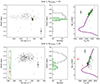 |
Fig. 2. Diagnostic RV–[Fe/H] plane, metallicity histogram and Kiel diagram used to isolate cluster members for Gran 1 (upper row) and Gran 4 (lower row). Left panels: RV–[Fe/H] plane for all the MUSE-extracted stars in the Gran 1 and Gran 4 fields. The box was drawn to select the cluster members using the individual RV and metallicity values. Red crosses represent stars outside the calibration parameter space, i.e. stars in the RGB tip or HB/SGB stars, the RV of which coincides with the one derived for the cluster, but with no reliable stellar atmospheric parameter determination. Middle panels: metallicity histogram for cluster-selected stars. The highlighted hatched-filled histogram contains the cluster members with reliable metallicity measurements within the box. Right panels: Kiel diagram for the field and cluster stars in grey and green, respectively. A PARSEC isochrone was drawn using the same derived metallicity with an age of 10 Gyr. Number of members considers all the valid RV cluster stars, i.e., members within the highlighted box. The error bar located in each panel represents the mean uncertainty for each corresponding parameter. |
As we mentioned earlier, we calibrated our AMBRE grid targeting only GC RGB stars, leaving other evolutionary stages without proper calibration. The calibration is evident when comparing the RGB sequence of the cluster with the 10 Gyr cluster mean metallicity PARSEC (Bressan et al. 2012; Marigo et al. 2013) isochrones. For this reason, the surface parameters derived from HB or SGB/BS stars (red crosses) are affected by more significant errors, as shown in Fig. 2. Nonetheless, when selecting cluster RGB stars (green dots and hatched histogram), the spread is minor, allowing us to assign a mean metallicity of [Fe/H]∼ − 1.7 to Gran 4, in perfect agreement with the results by Pace et al. (2023), which we discuss in Sect. 5.
3.2. Confirmation of Gran 4
Given the well-defined sequences in the CMD of Gran 4 (see Fig. 3 and Gran et al. 2022) and especially the extended HB and its low metallicity and RV well outside the distribution of field stars the identification of cluster members was straightforward. We used the 26 isolated spectroscopic members of Gran 4 and matched their coordinates (1 arcsec radius) to the Gaia DR3 catalogue. In total, 14 stars agree with the cluster RV and PM centroids. Considering individual measurement errors, we derived a weighted mean RV and metallicity of −265.28 ± 3.92 km s−1 and −1.72 ± 0.32 dex, respectively, using 1σ uncertainties. These values agree with a mono-metallic stellar population, for which we can confirm that Gran 4 is indeed a real GC. Figure 3 shows the MUSE and Gaia-VVV CMDs for this cluster decontaminated from field stars by means of both PMs and RVs using optical and near-IR filters.
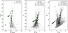 |
Fig. 3. CMDs of Gran 4 using different filters and catalogues. Left panel: MUSE CMD of cluster, containing field stars in the MUSE field of view (background points) and cluster members selected by their RVs (green circles). Middle panel: optical Gaia CMD comprising 2 arcmin within the cluster centre. Field stars are shown as background grey points, PM-cleaned members are shown as black points, RV and PM-selected cluster stars are given as green circles, while RV-only members (i.e. faint to have PM measurements) are shown as purple squares. Right panel: same as middle panel with an optical-near-IR CMD. We note that, for some stars, especially at the faint-end, there are no measured BP or RP-band magnitudes, resulting in a lower number of cluster stars in the CMDs. |
4. Milky Way globular cluster completeness and initial mass limit of bulge globular clusters
4.1. Globular cluster completeness behind the Galactic bulge/plane
Recently, multiple efforts have been made to estimate the total number of GCs bound to the Galaxy and, consequently, the number of clusters still to be discovered within the MW. Usually, the main focus is on the distant halo clusters (Contenta et al. 2017; Webb & Carlberg 2021, and references therein), assuming completeness of the GC population within galactocentric distances confined to R ≤ 20 − 50 kpc. Only a few studies have questioned the completeness of the number of clusters on the other side of the Galaxy (Ryu & Lee 2018) or presented the detection and survival issues of GCs buried in the bulge (Minniti et al. 2017, 2021a).
The clusters presented in this work and other recently confirmed GCs in the inner MW (Garro et al. 2020; Pace et al. 2023) challenge the assumption of 100% completeness towards the Galactic bulge. In what follows, we qualitatively estimate the number of missing GCs within galactocentric distances smaller than 20 kpc and then combine that number with previous halo predictions. By adding Gran 4, RLGC 1 and 2, and Garro 1 (Ryu & Lee 2018; Garro et al. 2020) to the compilation of March 2023 update of Baumgardt & Vasiliev (2021), we can give first-order estimates of the missing GCs at the far side of the Galaxy. To do this, we considered and adopted the Galactic bar as a symmetry axis and assumed that GCs are homogeneously distributed within the MW and that a Poisson distribution can model the number of GCs. This assumption is a first-order approximation of the observed GC distribution that exhibits a more complex structure (Arakelyan et al. 2018).
Figure 4 shows the adopted division to analyse the completeness of the GC population in four regions with an artistic representation of the Galaxy in the background3. In each of them (A, B, C, and D), there are 58, 24, 31, and 31 known GCs, respectively. In total, 144 GCs are located at galactocentric distances smaller than 20 kpc. As expected, a higher number of known GCs are located near the Sun in sector A, while roughly the same number of GCs are observed within Poisson errors (i.e.  ) in sectors B and D.
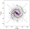 |
Fig. 4. Face-on artistic representation of MW within the inner 20 kpc. The Sun is at (8, 0) kpc and the known GCs are indicated with ⊙ and purple filled circles, respectively. Reference lines are drawn to show the analysed areas (A, B, C and D), considering the Galactic bar as a symmetry axis (i.e., dashed line from top left to bottom right). |
Assuming that the existing GCs are distributed isotropically, we can estimate the number of missing clusters in sector C by comparing it with the expected number of clusters observed on the near side of the MW. For both areas to be statistically similar (1σ error bars), the number of missing clusters should be more than 12 and less than 26. Given the extensive observations on our side of the Galaxy (i.e. shaded area A), we can almost completely rule out the possibility of number variations in that sector (i.e. undiscovered GC near the Sun).
We repeated the above exercise by (1) counting only GCs currently located close to the plane (|Z|< 1.5 kpc) and (2) limiting Zmax ≤ 3.5 kpc. The results give a similar number of ∼11−22 missing GCs. Adding previous estimations of missing GCs in the halo (Contenta et al. 2017; Webb & Carlberg 2021), the combined number of undiscovered clusters reaches up to a mean value of ∼22 GCs ((12 + 26)/2 = 19 behind the Galactic bulge/bar/disc and 3 in the halo).
The number presented above represents a first approximation of the actual value that is certainly affected by the violent dynamical processes dominating the early build-up history of the MW. In the more recent past of our Galaxy, only passages through the bar, the bulge, and the disc might significantly affect the chance of survival of a GC.
4.2. Observational globular cluster mass limit across the Galaxy
Also relevant to the present discussion is the minimum cluster mass that a GC should have in ordet to survive and be detected nowadays. Obviously, the observed GC mass function varies dramatically from the inner MW to the distant halo. With only a few GCs missing from the halo, the detection threshold was pushed down to ∼103 M⊙ (see Madore & Arp 1982; Abell 1955; Carraro 2005). However, this is one order of magnitude smaller than the mass of the smallest GC detected towards the inner Galaxy.
Complex dynamical processes that occur within the Galaxy, including but not limited to two-body relaxation, tidal truncation, disc/bulge shocks, cluster mass loss, dynamical friction and changes in the Galactic potential, create this natural inner-to-outer mass difference (see Murali & Weinberg 1997; Baumgardt & Makino 2003; Kruijssen et al. 2012; Carlberg & Keating 2022; Ishchenko et al. 2023, and references therein). Most of the processes listed above occur when GCs are embedded in a dense environment or pass through the disc/bulge along their orbits. Recent dynamical analyses of GCs have been performed that carefully take these processes into account (e.g., Baumgardt et al. 2019; Hughes et al. 2020; Ferrone et al. 2023); therefore, we can translate their results by searching for a lower limit on the GC bulge population.
Using the March 2023 update of the Baumgardt & Vasiliev (2021) catalogue, we were able to construct Fig. 5, which shows the initial and current GC masses for the entire MW GC population as a function of galactocentric radius (R). A similar figure was presented in Baumgardt et al. (2019, see their Fig. 7) but using the semi-major axis instead of R. Figure 5 also includes the maximum z extension (i.e., zmax) as a colour-coded third dimension. We adopted an uncertainty of 25% of the cluster total mass (i.e. σCurrent Mass = 0.25 × MCurrent) in case mass uncertainties were missing from the catalogue.
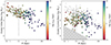 |
Fig. 5. Initial (left panel) and current (right panel) GC masses as a function of spherical galactocentric radius (R), colour-codded by their Zmax. The vertical line at 3.5 kpc is the estimated radius of the Galactic bulge. The grey hatched area in the right panel highlights the region where no GC has been discovered, implying an observational limit on the mass and orbital configuration below which GCs are more efficiently disrupted by the dynamical processes in the MW. The clusters analysed in this work are highlighted by squares in both panels. They are, in order of increasing R, Gran 1, 5, 3, 2, and 4. The right panel also contains the initial cluster masses derived by Baumgardt et al. (2019) as grey background points, as a reference for the initial-to-final mass ratio of the GCs. |
Observationally, clear differences arise using R in the x-axis in this figure. First, it is easier to identify the bulge region using R < 3.5 kpc, as suggested by Rojas-Arriagada et al. (2020); this could perhaps be extended up to ∼6 kpc. In this area, as pointed out by Baumgardt et al. (2019), dynamical processes determine a larger Minitial to Mcurrent mass differences, as low-mass clusters (∼104 M⊙) are more easily disrupted. The halo region also shows a distinct pattern, given the lower mass loss of clusters and the lower mass observable limit of ∼103 M⊙ hitherto, possibly due to a different origin of these outer GCs.
We can extend this analysis by including the newly discovered GCs. We can also extend the relationship to the Galactic disc, based on R. By comparing the mean mass-loss shift from GCs at the same radius, we derive a rough estimate for the initial mass of Gran 4 to be ∼106 M⊙. Initial masses for the remaining clusters were already derived in the Baumgardt et al. (2019) catalogue. A bulge/disc disruption region is hatched in grey in Fig. 5, highlighting the observational lack of clusters. We note that this area does not imply that GCs cannot exist in that part of the parameter space, simply that observations show no clusters in that area. A simple linear function M(R)∼104 R−1 (M⊙ kpc−1) was used to separate the parameter space in which GCs are observed. This functional form is valid from R ∼ 0.6 kpc (Gran 1) until the edge of the MW disc at ∼18 kpc (Gaia Collaboration 2021), in which no GC has been observed below this threshold to date.
5. Discussion and conclusions
As a follow-up to our previous work (Gran et al. 2022), we derived a mean radial velocity and metallicity for the cluster Gran 4 and updated the values derived for Gran 1, 2, 3, and 5. Although we analysed the same MUSE data as in Gran et al. (2022), we have now used the entire MUSE wavelength range rather than only two CaT lines, and we also upgraded the PMs by using the Gaia DR3 catalogue.
Overall, we find an excellent agreement with previous studies of these clusters, with just a few key differences. Fernández-Trincado et al. (2022) derived a much lower metallicity for Gran 3 and a different RV for this cluster. We notice the same trend in the more recent study of Pace et al. (2023). This issue was corrected when re-analysing the MUSE spectra, due to an incorrect air-to-vacuum wavelength calibration used in Gran et al. (2022), which led to that discrepancy of an ∼20 km s−1 shift between our previous results and those of Pace et al. (2023). Considering the metallicity dispersion, our derived RV and metallicity for Gran 3 (91.57 km s−1 and −1.63 dex, respectively, see Table 2), show remarkable similarity to the ones reported by Fernández-Trincado et al. (2022; ∼ − 1.7 dex and 95.9 km s−1) and Pace et al. (2023; −1.84 dex and 90.9 km s−1). Finally, in the case of Gran 4, we derive an RV and metallicity of [Fe/H] = −1.72 dex and RV = −265.3 km s−1, respectively, which are compatible, within errors, with the ones derived in by Pace et al. (2023) (i.e. [Fe/H] = −1.84 dex and RV = −266.4 km s−1). These values agree with the conclusions presented in Pace et al. (2023) stating that Gran 4 is part of the LMS/Wukong merger (Conroy et al. 2019; Naidu et al. 2020; Malhan et al. 2021) or the Helmi stream (Helmi et al. 1999).
Our analysis has proven that Gran 4 is a bona fide GC, previously hidden behind a highly crowded and reddened region towards the Galactic bulge. An initial mass of ∼106 M⊙ was assigned to the cluster based on the Minitial/Mcurrent ratio of clusters at a similar galactocentric radius. Furthermore, we present RVs and stellar atmospheric parameters for most of their observed members in a field of view of 1 sq. arcmin from the centre. Future planned high-resolution follow-ups will show whether or not the presented GCs host multiple stellar populations.
How many GCs are still missing on the far side of the Galaxy is still uncertain, and locating new GCs is challenging as a result of the high stellar density and reddening towards the Galactic bulge/plane. Despite the fact that our best estimation of ∼12 − 26 GCs is still to be discovered, the number heavily relies on critical assumptions such as symmetry and cluster survival rate. However, substantial progress has been achieved in the last few years thanks to the release of the Gaia DR3 catalogue (Gaia Collaboration 2023) and the improvement in the performances of near-IR detectors.
Recently, other stellar tracers have been used as well, shedding light on the spiral structure (Sanna et al. 2017; Minniti et al. 2020, 2021b), taking advantage of low-extinction windows (Saito et al. 2020), and using a variety of distance indicators (Hey et al. 2023) to map the other side of the Galaxy. GCs behind the bulge have been discovered and confirmed using joint observations, a number that will only increase with future Gaia DRs.
The promising new generation stellar surveys such as WEAVE (Jin et al. 2023), 4MOST (de Jong et al. 2019; Lucatello et al. 2023), and MOONS (Cirasuolo et al. 2020; Gonzalez et al. 2020), in addition to the augmented instrumental and observational capabilities of future facilities, for example Vera Rubin (Ivezić et al. 2019) and Gaia-NIR (Hobbs et al. 2016), will significantly increase our overall understanding of the MW and its GCs, expanding well-observed clusters towards the plane.
Image provided in the python package MW-plot. Documentation can be found at https://milkyway-plot.readthedocs.io
Acknowledgments
We gratefully thank Patrick de Laverny for providing access to the AMBRE synthetic spectra. F.G., G.K. and V.H. gratefully acknowledge support from the French National Research Agency (ANR) funded project “MWDisc” (ANR-20-CE31-0004) and “Pristine” (ANR-18-CE31-0017). This work was the last part of the Ph.D. thesis of FG, funded by grant CONICYT-PCHA Doctorado Nacional 2017-21171485. M.Z. acknowledges support from FONDECYT Regular grant No. 1230731. A.R.A. acknowledges support from FONDECYT through grant 3180203. J.A.C.-B. acknowledges support from FONDECYT Regular No. 1220083. E.V. acknowledges the Excellence Cluster ORIGINS Funded by the Deutsche Forschungsgemeinschaft (DFG, German Research Foundation) under Germany’s Excellence Strategy – EXC-2094-390783311. Support for M.Z., A.R.A., R.C., and M.D.L. is provided by the Ministerio de Ciencia, Tecnología, Conocimiento e Innovación/Agencia Nacional de Investigación y Desarrollo (ANID) Programa Iniciativa Científica Milenio through grant IC120009, awarded to the Millennium Institute of Astrophysics (M.A.S.) and the ANID BASAL Center for Astrophysics and Associated Technologies (CATA) through grant FB210003. We gratefully acknowledge the use of data from the VVV ESO Public Survey program ID 179.B-2002 taken with the VISTA telescope, and data products from the Cambridge Astronomical Survey Unit (CASU). The VVV Survey data are made public at the ESO Archive. Based on observations taken within the ESO VISTA Public Survey VVV, Program ID 179.B-2002. This work has made use of data from the European Space Agency (ESA) mission Gaia (https://www.cosmos.esa.int/gaia), processed by the Gaia Data Processing and Analysis Consortium (DPAC, https://www.cosmos.esa.int/web/gaia/dpac/consortium). Funding for the DPAC has been provided by national institutions, in particular the institutions participating in the Gaia Multilateral Agreement. This research has made use of the VizieR catalogue access tool, CDS, Strasbourg, France (DOI: 10.26093/cds/vizier). The original description of the VizieR service was published in Ochsenbein et al. (2000). This research made use of: TOPCAT (Taylor 2005), IPython/Jupyter (Pérez & Granger 2007; Kluyver et al. 2016), numpy (Harris et al. 2020), matplotlib (Hunter 2007), Astropy, a community developed core Python package for Astronomy (Astropy Collaboration 2013, 2018, 2022), Photutils, an Astropy package for detection and photometry of astronomical sources (Bradley et al. 2023), galpy: A Python Library for Galactic Dynamics (Bovy 2015), specutils (Earl et al. 2021), gala (Price-Whelan 2017; Price-Whelan et al. 2020), and Uncertainties: a Python package for calculations with uncertainties (Eric O. LEBIGOT, http://pythonhosted.org/uncertainties/). This research has made use of NASA’s Astrophysics Data System.
References
- Abell, G. O. 1955, PASP, 67, 258 [NASA ADS] [CrossRef] [Google Scholar]
- Arakelyan, N. R., Pilipenko, S. V., & Libeskind, N. I. 2018, MNRAS, 481, 918 [NASA ADS] [CrossRef] [Google Scholar]
- Astropy Collaboration (Robitaille, T. P., et al.) 2013, A&A, 558, A33 [NASA ADS] [CrossRef] [EDP Sciences] [Google Scholar]
- Astropy Collaboration (Price-Whelan, A. M., et al.) 2018, AJ, 156, 123 [Google Scholar]
- Astropy Collaboration (Price-Whelan, A. M., et al.) 2022, ApJ, 935, 167 [NASA ADS] [CrossRef] [Google Scholar]
- Bacon, R., Accardo, M., Adjali, L., et al. 2010, SPIE Conf. Ser., 7735, 773508 [Google Scholar]
- Bailin, J. 2019, ApJS, 245, 5 [NASA ADS] [CrossRef] [Google Scholar]
- Bailin, J., & von Klar, R. 2022, ApJ, 925, 36 [NASA ADS] [CrossRef] [Google Scholar]
- Bastian, N., & Lardo, C. 2018, ARA&A, 56, 83 [Google Scholar]
- Baumgardt, H., & Makino, J. 2003, MNRAS, 340, 227 [NASA ADS] [CrossRef] [Google Scholar]
- Baumgardt, H., & Vasiliev, E. 2021, MNRAS, 505, 5957 [NASA ADS] [CrossRef] [Google Scholar]
- Baumgardt, H., Hilker, M., Sollima, A., & Bellini, A. 2019, MNRAS, 482, 5138 [Google Scholar]
- Bovy, J. 2015, ApJS, 216, 29 [NASA ADS] [CrossRef] [Google Scholar]
- Bradley, L., Sipőcz, B., Robitaille, T., et al. 2022, https://doi.org/10.5281/zenodo.6825092 [Google Scholar]
- Bradley, L., Sipőcz, B., Robitaille, T., et al. 2023, https://doi.org/10.5281/zenodo.7946442 [Google Scholar]
- Bragaglia, A. 2018, in Astrometry and Astrophysics in the Gaia Sky, eds. A. Recio-Blanco, P. de Laverny, A. G. A. Brown, & T. Prusti, 330, 119 [NASA ADS] [Google Scholar]
- Bressan, A., Marigo, P., Girardi, L., et al. 2012, MNRAS, 427, 127 [NASA ADS] [CrossRef] [Google Scholar]
- Brodie, J. P., & Strader, J. 2006, ARA&A, 44, 193 [Google Scholar]
- Callingham, T. M., Cautun, M., Deason, A. J., et al. 2022, MNRAS, 513, 4107 [NASA ADS] [CrossRef] [Google Scholar]
- Cantat-Gaudin, T. 2022, Universe, 8, 111 [NASA ADS] [CrossRef] [Google Scholar]
- Cantat-Gaudin, T., & Anders, F. 2020, A&A, 633, A99 [NASA ADS] [CrossRef] [EDP Sciences] [Google Scholar]
- Cantat-Gaudin, T., Krone-Martins, A., Sedaghat, N., et al. 2019, A&A, 624, A126 [NASA ADS] [CrossRef] [EDP Sciences] [Google Scholar]
- Cantat-Gaudin, T., Anders, F., Castro-Ginard, A., et al. 2020, A&A, 640, A1 [NASA ADS] [CrossRef] [EDP Sciences] [Google Scholar]
- Carlberg, R. G., & Keating, L. C. 2022, ApJ, 924, 77 [NASA ADS] [CrossRef] [Google Scholar]
- Carraro, G. 2005, ApJ, 621, L61 [NASA ADS] [CrossRef] [Google Scholar]
- Castro-Ginard, A., Jordi, C., Luri, X., et al. 2018, A&A, 618, A59 [NASA ADS] [CrossRef] [EDP Sciences] [Google Scholar]
- Castro-Ginard, A., Jordi, C., Luri, X., et al. 2020, A&A, 635, A45 [NASA ADS] [CrossRef] [EDP Sciences] [Google Scholar]
- Castro-Ginard, A., Jordi, C., Luri, X., et al. 2022, A&A, 661, A118 [NASA ADS] [CrossRef] [EDP Sciences] [Google Scholar]
- Choi, J., Conroy, C., Ting, Y.-S., et al. 2018, ApJ, 863, 65 [NASA ADS] [CrossRef] [Google Scholar]
- Cirasuolo, M., Fairley, A., Rees, P., et al. 2020, The Messenger, 180, 10 [NASA ADS] [Google Scholar]
- Conroy, C., Bonaca, A., Cargile, P., et al. 2019, ApJ, 883, 107 [NASA ADS] [CrossRef] [Google Scholar]
- Contenta, F., Gieles, M., Balbinot, E., & Collins, M. L. M. 2017, MNRAS, 466, 1741 [NASA ADS] [CrossRef] [Google Scholar]
- Contreras Ramos, R., Zoccali, M., Rojas, F., et al. 2017, A&A, 608, A140 [NASA ADS] [CrossRef] [EDP Sciences] [Google Scholar]
- de Jong, R. S., Agertz, O., Berbel, A. A., et al. 2019, The Messenger, 175, 3 [NASA ADS] [Google Scholar]
- de Laverny, P., Recio-Blanco, A., Worley, C. C., & Plez, B. 2012, A&A, 544, A126 [NASA ADS] [CrossRef] [EDP Sciences] [Google Scholar]
- de Laverny, P., Recio-Blanco, A., Worley, C. C., et al. 2013, The Messenger, 153, 18 [NASA ADS] [Google Scholar]
- Earl, N., Tollerud, E., Jones, C., et al. 2021, https://doi.org/10.5281/zenodo.4603801 [Google Scholar]
- Fernández-Trincado, J. G., Minniti, D., Garro, E. R., & Villanova, S. 2022, A&A, 657, A84 [NASA ADS] [CrossRef] [EDP Sciences] [Google Scholar]
- Ferrone, S., Di Matteo, P., Mastrobuono-Battisti, A., et al. 2023, A&A, 673, A44 [NASA ADS] [CrossRef] [EDP Sciences] [Google Scholar]
- Forbes, D. A., & Bridges, T. 2010, MNRAS, 404, 1203 [NASA ADS] [Google Scholar]
- Forbes, D. A., Bastian, N., Gieles, M., et al. 2018, Proc. R. Soc. London Ser. A, 474, 20170616 [Google Scholar]
- Foreman-Mackey, D., Hogg, D. W., Lang, D., & Goodman, J. 2013, PASP, 125, 306 [Google Scholar]
- Gaia Collaboration (Prusti, T., et al.) 2016, A&A, 595, A1 [NASA ADS] [CrossRef] [EDP Sciences] [Google Scholar]
- Gaia Collaboration (Brown, A. G. A., et al.) 2018, A&A, 616, A1 [NASA ADS] [CrossRef] [EDP Sciences] [Google Scholar]
- Gaia Collaboration (Antoja, T., et al.) 2021, A&A, 649, A8 [EDP Sciences] [Google Scholar]
- Gaia Collaboration (Vallenari, A., et al.) 2023, A&A, 674, A1 [NASA ADS] [CrossRef] [EDP Sciences] [Google Scholar]
- Garro, E. R., Minniti, D., Gómez, M., et al. 2020, A&A, 642, L19 [EDP Sciences] [Google Scholar]
- Garro, E. R., Minniti, D., Alessi, B., et al. 2022a, A&A, 659, A155 [NASA ADS] [CrossRef] [EDP Sciences] [Google Scholar]
- Garro, E. R., Minniti, D., Gómez, M., et al. 2022b, A&A, 662, A95 [NASA ADS] [CrossRef] [EDP Sciences] [Google Scholar]
- Gonzalez, O. A., Mucciarelli, A., Origlia, L., et al. 2020, The Messenger, 180, 18 [NASA ADS] [Google Scholar]
- Gran, F., Zoccali, M., Contreras Ramos, R., et al. 2019, A&A, 628, A45 [NASA ADS] [CrossRef] [EDP Sciences] [Google Scholar]
- Gran, F., Zoccali, M., Saviane, I., et al. 2022, MNRAS, 509, 4962 [Google Scholar]
- Gratton, R., Sneden, C., & Carretta, E. 2004, ARA&A, 42, 385 [Google Scholar]
- Gratton, R., Bragaglia, A., Carretta, E., et al. 2019, A&ARv, 27, 8 [Google Scholar]
- Hammer, F., Li, H., Mamon, G. A., et al. 2023, MNRAS, 519, 5059 [CrossRef] [Google Scholar]
- Harris, W. E., & Racine, R. 1979, ARA&A, 17, 241 [NASA ADS] [CrossRef] [Google Scholar]
- Harris, C. R., Millman, K. J., van der Walt, S. J., et al. 2020, Nature, 585, 357 [NASA ADS] [CrossRef] [Google Scholar]
- Hartke, J., Kakkad, D., Reyes, C., et al. 2020, SPIE Conf. Ser., 11448, 114480V [NASA ADS] [Google Scholar]
- He, Z.-H., Xu, Y., Hao, C.-J., Wu, Z.-Y., & Li, J.-J. 2021, Res. Astron. Astrophys., 21, 093 [Google Scholar]
- He, Z., Wang, K., Luo, Y., et al. 2022, ApJS, 262, 7 [NASA ADS] [CrossRef] [Google Scholar]
- He, Z., Liu, X., Luo, Y., Wang, K., & Jiang, Q. 2023, ApJS, 264, 8 [NASA ADS] [CrossRef] [Google Scholar]
- Helmi, A., White, S. D. M., de Zeeuw, P. T., & Zhao, H. 1999, Nature, 402, 53 [Google Scholar]
- Hey, D. R., Huber, D., Shappee, B. J., et al. 2023, AJ, 166, 249 [NASA ADS] [CrossRef] [Google Scholar]
- Hobbs, D., Høg, E., Mora, A., et al. 2016, arXiv e-prints [arXiv:1609.07325] [Google Scholar]
- Huang, K.-W., & Koposov, S. E. 2021, MNRAS, 500, 986 [Google Scholar]
- Hughes, M. E., Pfeffer, J. L., Martig, M., et al. 2020, MNRAS, 491, 4012 [NASA ADS] [CrossRef] [Google Scholar]
- Hunt, E. L., & Reffert, S. 2021, A&A, 646, A104 [NASA ADS] [CrossRef] [EDP Sciences] [Google Scholar]
- Hunt, E. L., & Reffert, S. 2023, A&A, 673, A114 [NASA ADS] [CrossRef] [EDP Sciences] [Google Scholar]
- Hunter, J. D. 2007, Comput. Sci. Eng., 9, 90 [NASA ADS] [CrossRef] [Google Scholar]
- Husser, T.-O., Latour, M., Brinchmann, J., et al. 2020, A&A, 635, A114 [NASA ADS] [CrossRef] [EDP Sciences] [Google Scholar]
- Ishchenko, M., Sobolenko, M., Berczik, P., et al. 2023, A&A, 673, A152 [NASA ADS] [CrossRef] [EDP Sciences] [Google Scholar]
- Ivezić, Ž., Kahn, S. M., Tyson, J. A., et al. 2019, ApJ, 873, 111 [Google Scholar]
- Jin, S., Trager, S. C., Dalton, G. B., et al. 2023, MNRAS, in press, https://doi.org/10.1093/mnras/stad557 [Google Scholar]
- Kluyver, T., Ragan-Kelley, B., Pérez, F., et al. 2016, in Positioning and Power in Academic Publishing: Players, Agents and Agendas, eds. F. Loizides, & B. Schmidt (IOS Press), 87 [Google Scholar]
- Koposov, S. E., Belokurov, V., & Torrealba, G. 2017, MNRAS, 470, 2702 [NASA ADS] [CrossRef] [Google Scholar]
- Kruijssen, J. M. D., Maschberger, T., Moeckel, N., et al. 2012, MNRAS, 419, 841 [NASA ADS] [CrossRef] [Google Scholar]
- Kruijssen, J. M. D., Pfeffer, J. L., Crain, R. A., & Bastian, N. 2019a, MNRAS, 486, 3134 [NASA ADS] [CrossRef] [Google Scholar]
- Kruijssen, J. M. D., Pfeffer, J. L., Reina-Campos, M., Crain, R. A., & Bastian, N. 2019b, MNRAS, 486, 3180 [Google Scholar]
- Leaman, R., VandenBerg, D. A., & Mendel, J. T. 2013, MNRAS, 436, 122 [Google Scholar]
- Lucatello, S., Bragaglia, A., Vallenari, A., et al. 2023, The Messenger, 190, 13 [NASA ADS] [Google Scholar]
- Madore, B. F., & Arp, H. C. 1982, PASP, 94, 40 [NASA ADS] [CrossRef] [Google Scholar]
- Malhan, K., Yuan, Z., Ibata, R. A., et al. 2021, ApJ, 920, 51 [NASA ADS] [CrossRef] [Google Scholar]
- Marigo, P., Bressan, A., Nanni, A., Girardi, L., & Pumo, M. L. 2013, MNRAS, 434, 488 [Google Scholar]
- Marín-Franch, A., Aparicio, A., Piotto, G., et al. 2009, ApJ, 694, 1498 [Google Scholar]
- Massari, D., Koppelman, H. H., & Helmi, A. 2019, A&A, 630, L4 [NASA ADS] [CrossRef] [EDP Sciences] [Google Scholar]
- Minniti, D., Lucas, P. W., Emerson, J. P., et al. 2010, New Astron., 15, 433 [Google Scholar]
- Minniti, D., Geisler, D., Alonso-García, J., et al. 2017, ApJ, 849, L24 [CrossRef] [Google Scholar]
- Minniti, J. H., Sbordone, L., Rojas-Arriagada, A., et al. 2020, A&A, 640, A92 [EDP Sciences] [Google Scholar]
- Minniti, D., Fernández-Trincado, J. G., Smith, L. C., et al. 2021a, A&A, 648, A86 [NASA ADS] [CrossRef] [EDP Sciences] [Google Scholar]
- Minniti, J. H., Zoccali, M., Rojas-Arriagada, A., et al. 2021b, A&A, 654, A138 [NASA ADS] [CrossRef] [EDP Sciences] [Google Scholar]
- Murali, C., & Weinberg, M. D. 1997, MNRAS, 288, 749 [NASA ADS] [CrossRef] [Google Scholar]
- Myeong, G. C., Vasiliev, E., Iorio, G., Evans, N. W., & Belokurov, V. 2019, MNRAS, 488, 1235 [Google Scholar]
- Naidu, R. P., Conroy, C., Bonaca, A., et al. 2020, ApJ, 901, 48 [Google Scholar]
- Ness, M., Hogg, D. W., Rix, H. W., Ho, A. Y. Q., & Zasowski, G. 2015, ApJ, 808, 16 [NASA ADS] [CrossRef] [Google Scholar]
- Nidever, D. 2021, https://doi.org/10.5281/zenodo.4906681 [Google Scholar]
- Ochsenbein, F., Bauer, P., & Marcout, J. 2000, A&AS, 143, 23 [NASA ADS] [CrossRef] [EDP Sciences] [Google Scholar]
- Pace, A. B., Koposov, S. E., Walker, M. G., et al. 2023, MNRAS, 526, 1075 [CrossRef] [Google Scholar]
- Pagnini, G., Di Matteo, P., Khoperskov, S., et al. 2023, A&A, 673, A86 [NASA ADS] [CrossRef] [EDP Sciences] [Google Scholar]
- Pérez, F., & Granger, B. E. 2007, Comput. Sci. Eng., 9, 21 [Google Scholar]
- Price-Whelan, A. M. 2017, J. Open Source Softw., 2, 388 [NASA ADS] [CrossRef] [Google Scholar]
- Price-Whelan, A., Sipőcz, B., Lenz, D., et al. 2020, https://doi.org/10.5281/zenodo.4159870 [Google Scholar]
- Recio-Blanco, A. 2018, A&A, 620, A194 [NASA ADS] [CrossRef] [EDP Sciences] [Google Scholar]
- Renzini, A. 2017, MNRAS, 469, L63 [Google Scholar]
- Rojas-Arriagada, A., Zasowski, G., Schultheis, M., et al. 2020, MNRAS, 499, 1037 [Google Scholar]
- Ryu, J., & Lee, M. G. 2018, ApJ, 863, L38 [NASA ADS] [CrossRef] [Google Scholar]
- Saito, R. K., Minniti, D., Benjamin, R. A., et al. 2020, MNRAS, 494, L32 [Google Scholar]
- Sanna, A., Reid, M. J., Dame, T. M., Menten, K. M., & Brunthaler, A. 2017, Science, 358, 227 [NASA ADS] [CrossRef] [Google Scholar]
- Smith, L. C., Lucas, P. W., Kurtev, R., et al. 2018, MNRAS, 474, 1826 [Google Scholar]
- Ströbele, S., La Penna, P., Arsenault, R., et al. 2012, SPIE Conf. Ser., 8447, 844737 [Google Scholar]
- Stuik, R., Bacon, R., Conzelmann, R., et al. 2006, New Astron. Rev., 49, 618 [CrossRef] [Google Scholar]
- Surot, F., Valenti, E., Hidalgo, S. L., et al. 2019, A&A, 623, A168 [NASA ADS] [CrossRef] [EDP Sciences] [Google Scholar]
- Taylor, M. B. 2005, ASP Conf. Ser., 347, 29 [Google Scholar]
- Vanzella, E., Calura, F., Meneghetti, M., et al. 2017, MNRAS, 467, 4304 [Google Scholar]
- Vasiliev, E., & Baumgardt, H. 2021, MNRAS, 505, 5978 [NASA ADS] [CrossRef] [Google Scholar]
- Wang, Z., Hayden, M. R., Sharma, S., et al. 2022, MNRAS, 514, 1034 [NASA ADS] [CrossRef] [Google Scholar]
- Watkins, L. L., van der Marel, R. P., Bellini, A., & Anderson, J. 2015, ApJ, 803, 29 [Google Scholar]
- Webb, J. J., & Carlberg, R. G. 2021, MNRAS, 502, 4547 [CrossRef] [Google Scholar]
- Weilbacher, P. M., Palsa, R., Streicher, O., et al. 2020, A&A, 641, A28 [NASA ADS] [CrossRef] [EDP Sciences] [Google Scholar]
Appendix A: Additional GC plots and complete membership catalogues
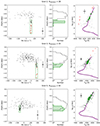 |
Fig. A.1. Diagnostic RV-[Fe/H] plane, metallicity histogram and Kiel diagram used to isolate cluster members for Gran 2 (upper row), Gran 3 (middle row) and Gran 5 (lower row). Left panels: RV-[Fe/H] plane for all the MUSE-extracted stars in the Gran 2 (upper row), Gran 3 (middle row) and Gran 5 (lower row) fields. The box was drawn to select the cluster members using the individual RV and metallicity values. Red crosses represent stars outside the calibration parameter space, i.e., stars in the RGB tip or HB/SGB stars, whose RV coincides with that derived for the cluster, but with no reliable stellar atmospheric parameter determination. Middle panels: Metallicity histogram for cluster-selected stars. The highlighted hatched-filled histogram contains the cluster members within the box. Right panels: Kiel diagram for field and cluster stars in grey and green, respectively. A PARSEC isochrone was drawn using the same derived metallicity with an age of 10 Gyr. The number of members considers all the valid RV cluster stars, i.e., members within the highlighted box. The error bar located in each panel represents the mean uncertainty for each corresponding parameter. |
Atmospheric parameters for all MUSE Gran 1 analysed stars. Star ID, coordinates, temperature, surface gravity, metallicity, RV, and mean S/N were derived for observed GC members based on their multi-dimensional membership (RV, [Fe/H], and Kiel diagram).
Atmospheric parameters for all MUSE Gran 2 analysed stars. Star ID, coordinates, temperature, surface gravity, metallicity, RV, and mean S/N were derived for observed GC members based on their multi-dimensional membership (RV, [Fe/H], and Kiel diagram).
Atmospheric parameters for all MUSE Gran 3 analysed stars. Star ID, coordinates, temperature, surface gravity, metallicity, RV, and mean S/N were derived for observed GC members based on their multi-dimensional membership (RV, [Fe/H], and Kiel diagram).
Atmospheric parameters for all MUSE Gran 4 analysed stars. Star ID, coordinates, temperature, surface gravity, metallicity, RV, and mean S/N were derived for observed GC members based on their multi-dimensional membership (RV, [Fe/H], and Kiel diagram).
Atmospheric parameters for all MUSE Gran 5 analysed stars. Star ID, coordinates, temperature, surface gravity, metallicity, RV, and mean S/N were derived for observed GC members based on their multi-dimensional membership (RV, [Fe/H], and Kiel diagram).
All Tables
Atmospheric parameters for all MUSE Gran 1 analysed stars. Star ID, coordinates, temperature, surface gravity, metallicity, RV, and mean S/N were derived for observed GC members based on their multi-dimensional membership (RV, [Fe/H], and Kiel diagram).
Atmospheric parameters for all MUSE Gran 2 analysed stars. Star ID, coordinates, temperature, surface gravity, metallicity, RV, and mean S/N were derived for observed GC members based on their multi-dimensional membership (RV, [Fe/H], and Kiel diagram).
Atmospheric parameters for all MUSE Gran 3 analysed stars. Star ID, coordinates, temperature, surface gravity, metallicity, RV, and mean S/N were derived for observed GC members based on their multi-dimensional membership (RV, [Fe/H], and Kiel diagram).
Atmospheric parameters for all MUSE Gran 4 analysed stars. Star ID, coordinates, temperature, surface gravity, metallicity, RV, and mean S/N were derived for observed GC members based on their multi-dimensional membership (RV, [Fe/H], and Kiel diagram).
Atmospheric parameters for all MUSE Gran 5 analysed stars. Star ID, coordinates, temperature, surface gravity, metallicity, RV, and mean S/N were derived for observed GC members based on their multi-dimensional membership (RV, [Fe/H], and Kiel diagram).
All Figures
|
Fig. 1. Extracted MUSE spectra and associated models for different parts of spectra of two high-S/N (> 110) stars: Gran 1 stars 010 and 012. In each panel, features in each region are highlighted. Two left panels for RGB star, and two right panels for HB star: Mgb around ∼5175 Å, Hα (6562 Å), CaT between ∼8400 − 8700 Å, and Paschen hydrogen series starting at ∼8450 Å. |
| In the text | |
|
Fig. 2. Diagnostic RV–[Fe/H] plane, metallicity histogram and Kiel diagram used to isolate cluster members for Gran 1 (upper row) and Gran 4 (lower row). Left panels: RV–[Fe/H] plane for all the MUSE-extracted stars in the Gran 1 and Gran 4 fields. The box was drawn to select the cluster members using the individual RV and metallicity values. Red crosses represent stars outside the calibration parameter space, i.e. stars in the RGB tip or HB/SGB stars, the RV of which coincides with the one derived for the cluster, but with no reliable stellar atmospheric parameter determination. Middle panels: metallicity histogram for cluster-selected stars. The highlighted hatched-filled histogram contains the cluster members with reliable metallicity measurements within the box. Right panels: Kiel diagram for the field and cluster stars in grey and green, respectively. A PARSEC isochrone was drawn using the same derived metallicity with an age of 10 Gyr. Number of members considers all the valid RV cluster stars, i.e., members within the highlighted box. The error bar located in each panel represents the mean uncertainty for each corresponding parameter. |
| In the text | |
|
Fig. 3. CMDs of Gran 4 using different filters and catalogues. Left panel: MUSE CMD of cluster, containing field stars in the MUSE field of view (background points) and cluster members selected by their RVs (green circles). Middle panel: optical Gaia CMD comprising 2 arcmin within the cluster centre. Field stars are shown as background grey points, PM-cleaned members are shown as black points, RV and PM-selected cluster stars are given as green circles, while RV-only members (i.e. faint to have PM measurements) are shown as purple squares. Right panel: same as middle panel with an optical-near-IR CMD. We note that, for some stars, especially at the faint-end, there are no measured BP or RP-band magnitudes, resulting in a lower number of cluster stars in the CMDs. |
| In the text | |
|
Fig. 4. Face-on artistic representation of MW within the inner 20 kpc. The Sun is at (8, 0) kpc and the known GCs are indicated with ⊙ and purple filled circles, respectively. Reference lines are drawn to show the analysed areas (A, B, C and D), considering the Galactic bar as a symmetry axis (i.e., dashed line from top left to bottom right). |
| In the text | |
|
Fig. 5. Initial (left panel) and current (right panel) GC masses as a function of spherical galactocentric radius (R), colour-codded by their Zmax. The vertical line at 3.5 kpc is the estimated radius of the Galactic bulge. The grey hatched area in the right panel highlights the region where no GC has been discovered, implying an observational limit on the mass and orbital configuration below which GCs are more efficiently disrupted by the dynamical processes in the MW. The clusters analysed in this work are highlighted by squares in both panels. They are, in order of increasing R, Gran 1, 5, 3, 2, and 4. The right panel also contains the initial cluster masses derived by Baumgardt et al. (2019) as grey background points, as a reference for the initial-to-final mass ratio of the GCs. |
| In the text | |
|
Fig. A.1. Diagnostic RV-[Fe/H] plane, metallicity histogram and Kiel diagram used to isolate cluster members for Gran 2 (upper row), Gran 3 (middle row) and Gran 5 (lower row). Left panels: RV-[Fe/H] plane for all the MUSE-extracted stars in the Gran 2 (upper row), Gran 3 (middle row) and Gran 5 (lower row) fields. The box was drawn to select the cluster members using the individual RV and metallicity values. Red crosses represent stars outside the calibration parameter space, i.e., stars in the RGB tip or HB/SGB stars, whose RV coincides with that derived for the cluster, but with no reliable stellar atmospheric parameter determination. Middle panels: Metallicity histogram for cluster-selected stars. The highlighted hatched-filled histogram contains the cluster members within the box. Right panels: Kiel diagram for field and cluster stars in grey and green, respectively. A PARSEC isochrone was drawn using the same derived metallicity with an age of 10 Gyr. The number of members considers all the valid RV cluster stars, i.e., members within the highlighted box. The error bar located in each panel represents the mean uncertainty for each corresponding parameter. |
| In the text | |
Current usage metrics show cumulative count of Article Views (full-text article views including HTML views, PDF and ePub downloads, according to the available data) and Abstracts Views on Vision4Press platform.
Data correspond to usage on the plateform after 2015. The current usage metrics is available 48-96 hours after online publication and is updated daily on week days.
Initial download of the metrics may take a while.