| Issue |
A&A
Volume 682, February 2024
|
|
|---|---|---|
| Article Number | L3 | |
| Number of page(s) | 15 | |
| Section | Letters to the Editor | |
| DOI | https://doi.org/10.1051/0004-6361/202348308 | |
| Published online | 01 February 2024 | |
Letter to the Editor
Ordered magnetic fields around the 3C 84 central black hole
1
Max-Planck-Institut für Radioastronomie, Auf dem Hügel 69, 53121 Bonn, Germany
e-mail: This email address is being protected from spambots. You need JavaScript enabled to view it.
2
Department of Astronomy and Atmospheric Sciences, Kyungpook National University, Daegu 702-701, Republic of Korea
3
Institute of Physics, Silesian University in Opava, Bezručovo nám. 13, 746 01 Opava, Czech Republic
4
Instituto de Astrofísica de Andalucía-CSIC, Glorieta de la Astronomía s/n, 18008 Granada, Spain
5
Institut de Radioastronomie Millimétrique (IRAM), Avenida Divina Pastora 7, Local 20, 18012 Granada, Spain
6
Department of Astrophysics, Institute for Mathematics, Astrophysics and Particle Physics (IMAPP), Radboud University, PO Box 9010 6500 GL Nijmegen, The Netherlands
7
Black Hole Initiative at Harvard University, 20 Garden Street, Cambridge, MA 02138, USA
8
Center for Astrophysics, Harvard & Smithsonian, 60 Garden Street, Cambridge, MA 02138, USA
9
Steward Observatory and Department of Astronomy, University of Arizona, 933 N. Cherry Ave., Tucson, AZ 85721, USA
10
Data Science Institute, University of Arizona, 1230 N. Cherry Ave., Tucson, AZ 85721, USA
11
Program in Applied Mathematics, University of Arizona, 617 N. Santa Rita, Tucson, AZ 85721, USA
12
NASA Hubble Fellowship Program, Einstein Fellow, USA
13
Massachusetts Institute of Technology Haystack Observatory, 99 Millstone Road, Westford, MA 01886, USA
14
National Astronomical Observatory of Japan, 2-21-1 Osawa, Mitaka, Tokyo 181-8588, Japan
15
Department of Physics, Faculty of Science, Universiti Malaya, 50603 Kuala Lumpur, Malaysia
16
Department of Physics & Astronomy, The University of Texas at San Antonio, One UTSA Circle, San Antonio, TX 78249, USA
17
Institute of Astronomy and Astrophysics, Academia Sinica, 11F of Astronomy-Mathematics Building, AS/NTU No. 1, Sec. 4, Roosevelt Rd., Taipei, 10617 Taiwan, R.O.C.
18
Departament d’Astronomia i Astrofísica, Universitat de València, C. Dr. Moliner 50, 46100 Burjassot, València, Spain
19
Observatori Astronòmic, Universitat de València, C. Catedrático José Beltrán 2, 46980 Paterna, València, Spain
20
Department of Space, Earth and Environment, Chalmers University of Technology, Onsala Space Observatory, 43992 Onsala, Sweden
21
Yale Center for Astronomy & Astrophysics, Yale University, 52 Hillhouse Avenue, New Haven, CT 06511, USA
22
Department of Physics, University of Illinois, 1110 West Green Street, Urbana, IL 61801, USA
23
Fermi National Accelerator Laboratory, MS209, PO Box 500 Batavia, IL 60510, USA
24
Department of Astronomy and Astrophysics, University of Chicago, 5640 South Ellis Avenue, Chicago, IL 60637, USA
25
East Asian Observatory, 660 N. A’ohoku Place, Hilo, HI 96720, USA
26
James Clerk Maxwell Telescope (JCMT), 660 N. A’ohoku Place, Hilo, HI 96720, USA
27
California Institute of Technology, 1200 East California Boulevard, Pasadena, CA 91125, USA
28
Institute of Astronomy and Astrophysics, Academia Sinica, 645 N. A’ohoku Place, Hilo, HI 96720, USA
29
Department of Physics and Astronomy, University of Hawaii at Manoa, 2505 Correa Road, Honolulu, HI 96822, USA
30
Department of Physics, McGill University, 3600 rue University, Montréal, QC H3A 2T8, Canada
31
Trottier Space Institute at McGill, 3550 rue University, Montréal, QC H3A 2A7, Canada
32
Institut de Radioastronomie Millimétrique (IRAM), 300 rue de la Piscine, 38406 Saint Martin d’Hères, France
33
Perimeter Institute for Theoretical Physics, 31 Caroline Street North, Waterloo, ON N2L 2Y5, Canada
34
Department of Physics and Astronomy, University of Waterloo, 200 University Avenue West, Waterloo, ON N2L 3G1, Canada
35
Waterloo Centre for Astrophysics, University of Waterloo, Waterloo, ON N2L 3G1, Canada
36
Department of Astronomy, University of Massachusetts, Amherst, MA 01003, USA
37
Korea Astronomy and Space Science Institute, Daedeok-daero 776, Yuseong-gu, Daejeon 34055, Republic of Korea
38
University of Science and Technology, Gajeong-ro 217, Yuseong-gu, Daejeon 34113, Republic of Korea
39
Kavli Institute for Cosmological Physics, University of Chicago, 5640 South Ellis Avenue, Chicago, IL 60637, USA
40
Department of Physics, University of Chicago, 5720 South Ellis Avenue, Chicago, IL 60637, USA
41
Enrico Fermi Institute, University of Chicago, 5640 South Ellis Avenue, Chicago, IL 60637, USA
42
Princeton Gravity Initiative, Jadwin Hall, Princeton University, Princeton, NJ 08544, USA
43
Cornell Center for Astrophysics and Planetary Science, Cornell University, Ithaca, NY 14853, USA
44
Shanghai Astronomical Observatory, Chinese Academy of Sciences, 80 Nandan Road, Shanghai 200030, PR China
45
Key Laboratory of Radio Astronomy, Chinese Academy of Sciences, Nanjing 210008, PR China
46
Physics Department, Fairfield University, 1073 North Benson Road, Fairfield, CT 06824, USA
47
Department of Astronomy, University of Illinois at Urbana-Champaign, 1002 West Green Street, Urbana, IL 61801, USA
48
Instituto de Astronomía, Universidad Nacional Autónoma de México (UNAM), Apdo Postal 70-264, Ciudad de México, Mexico
49
Institut für Theoretische Physik, Goethe-Universität Frankfurt, Max-von-Laue-Straße 1, 60438 Frankfurt am Main, Germany
50
Research Center for Intelligent Computing Platforms, Zhejiang Laboratory, Hangzhou 311100, PR China
51
Tsung-Dao Lee Institute, Shanghai Jiao Tong University, Shengrong Road 520, Shanghai 201210, PR China
52
Department of Astronomy and Columbia Astrophysics Laboratory, Columbia University, 500 W. 120th Street, New York, NY 10027, USA
53
Center for Computational Astrophysics, Flatiron Institute, 162 Fifth Avenue, New York, NY 10010, USA
54
Dipartimento di Fisica “E. Pancini”, Universitá di Napoli “Federico II”, Compl. Univ. di Monte S. Angelo, Edificio G, Via Cinthia, 80126 Napoli, Italy
55
INFN Sez. di Napoli, Compl. Univ. di Monte S. Angelo, Edificio G, Via Cinthia, 80126 Napoli, Italy
56
Wits Centre for Astrophysics, University of the Witwatersrand, 1 Jan Smuts Avenue, Braamfontein, Johannesburg 2050, South Africa
57
Department of Physics, University of Pretoria, Hatfield, Pretoria 0028, South Africa
58
Centre for Radio Astronomy Techniques and Technologies, Department of Physics and Electronics, Rhodes University, Makhanda 6140, South Africa
59
ASTRON, Oude Hoogeveensedijk 4, 7991 PD Dwingeloo, The Netherlands
60
LESIA, Observatoire de Paris, Université PSL, CNRS, Sorbonne Université, Université de Paris, 5 place Jules Janssen, 92195 Meudon, France
61
JILA and Department of Astrophysical and Planetary Sciences, University of Colorado, Boulder, CO 80309, USA
62
National Astronomical Observatories, Chinese Academy of Sciences, 20A Datun Road, Chaoyang District, Beijing 100101, PR China
63
Las Cumbres Observatory, 6740 Cortona Drive, Suite 102, Goleta, CA 93117-5575, USA
64
Department of Physics, University of California, Santa Barbara, CA 93106-9530, USA
65
National Radio Astronomy Observatory, 520 Edgemont Road, Charlottesville, VA 22903, USA
66
Department of Electrical Engineering and Computer Science, Massachusetts Institute of Technology, 32-D476, 77 Massachusetts Ave., Cambridge, MA 02142, USA
67
Google Research, 355 Main St., Cambridge, MA 02142, USA
68
Institut für Theoretische Physik und Astrophysik, Universität Würzburg, Emil-Fischer-Str. 31, 97074 Würzburg, Germany
69
Department of History of Science, Harvard University, Cambridge, MA 02138, USA
70
Department of Physics, Harvard University, Cambridge, MA 02138, USA
71
NCSA, University of Illinois, 1205 W. Clark St., Urbana, IL 61801, USA
72
Instituto de Astronomia, Geofísica e Ciências Atmosféricas, Universidade de São Paulo, R. do Matão, 1226, São Paulo, SP 05508-090, Brazil
73
Dipartimento di Fisica, Universitá degli Studi di Cagliari, SP Monserrato-Sestu km 0.7, 09042 Monserrato, (CA), Italy
74
INAF – Osservatorio Astronomico di Cagliari, Via della Scienza 5, 09047 Selargius (CA), Italy
75
INFN, sezione di Cagliari, 09042 Monserrato (CA), Italy
76
CP3-Origins, University of Southern Denmark, Campusvej 55, 5230 Odense M, Denmark
77
Instituto Nacional de Astrofísica, Óptica y Electrónica. Apartado Postal 51 y 216, 72000 Puebla Pue., Mexico
78
Consejo Nacional de Ciencia y Tecnología, Av. Insurgentes Sur 1582, 03940 Ciudad de México, México
79
Key Laboratory for Research in Galaxies and Cosmology, Chinese Academy of Sciences, Shanghai 200030, PR China
80
Mizusawa VLBI Observatory, National Astronomical Observatory of Japan, 2-12 Hoshigaoka, Mizusawa, Oshu, Iwate 023-0861, Japan
81
Department of Astronomical Science, The Graduate University for Advanced Studies (SOKENDAI), 2-21-1 Osawa, Mitaka, Tokyo 181-8588, Japan
82
Trottier Space Institute at McGill, 3550 rue University, Montréal, QC H3A 2A7, Canada
83
NOVA Sub-mm Instrumentation Group, Kapteyn Astronomical Institute, University of Groningen, Landleven 12, 9747 AD Groningen, The Netherlands
84
Department of Astronomy, School of Physics, Peking University, Beijing 100871, PR China
85
Kavli Institute for Astronomy and Astrophysics, Peking University, Beijing 100871, PR China
86
Department of Astronomy, Graduate School of Science, The University of Tokyo, 7-3-1 Hongo, Bunkyo-ku, Tokyo 113-0033, Japan
87
The Institute of Statistical Mathematics, 10-3 Midori-cho, Tachikawa, Tokyo 190-8562, Japan
88
Department of Statistical Science, The Graduate University for Advanced Studies (SOKENDAI), 10-3 Midori-cho, Tachikawa, Tokyo 190-8562, Japan
89
, 5-1-5 Kashiwanoha, Kashiwa 277-8583, Japan
90
Leiden Observatory, Leiden University, Postbus 2300, 9513 RA Leiden, The Netherlands
91
ASTRAVEO LLC, PO Box 1668, Gloucester, MA 01931, USA
92
, 35 Dory Road, Gloucester, MA 01930, USA
93
Institute for Astrophysical Research, Boston University, 725 Commonwealth Ave., Boston, MA 02215, USA
94
Institute for Cosmic Ray Research, The University of Tokyo, 5-1-5 Kashiwanoha, Kashiwa, Chiba 277-8582, Japan
95
Joint Institute for VLBI ERIC (JIVE), Oude Hoogeveensedijk 4, 7991 PD Dwingeloo, The Netherlands
96
Kogakuin University of Technology & Engineering, Academic Support Center, 2665-1 Nakano, Hachioji, Tokyo 192-0015, Japan
97
Graduate School of Science and Technology, Niigata University, 8050 Ikarashi 2-no-cho, Nishi-ku, Niigata 950-2181, Japan
98
Physics Department, National Sun Yat-Sen University, No. 70, Lien-Hai Road, Kaosiung City, 80424 Taiwan, R.O.C.
99
National Optical Astronomy Observatory, 950 N. Cherry Ave., Tucson, AZ 85719, USA
100
Department of Physics, The Chinese University of Hong Kong, Shatin, N. T., Hong Kong
101
School of Astronomy and Space Science, Nanjing University, Nanjing 210023, PR China
102
Key Laboratory of Modern Astronomy and Astrophysics, Nanjing University, Nanjing 210023, PR China
103
INAF-Istituto di Radioastronomia, Via P. Gobetti 101, 40129 Bologna, Italy
104
INAF-Istituto di Radioastronomia & Italian ALMA Regional Centre, Via P. Gobetti 101, 40129 Bologna, Italy
105
Department of Physics, National Taiwan University, No. 1, Sec. 4, Roosevelt Rd., Taipei, 10617 Taiwan, R.O.C.
106
Instituto de Radioastronomía y Astrofísica, Universidad Nacional Autónoma de México, Morelia 58089, Mexico
107
Yunnan Observatories, Chinese Academy of Sciences, 650011 Kunming, Yunnan Province, PR China
108
Center for Astronomical Mega-Science, Chinese Academy of Sciences, 20A Datun Road, Chaoyang District, Beijing 100012, PR China
109
Key Laboratory for the Structure and Evolution of Celestial Objects, Chinese Academy of Sciences, 650011 Kunming, PR China
110
Anton Pannekoek Institute for Astronomy, University of Amsterdam, Science Park 904, 1098 XH Amsterdam, The Netherlands
111
Gravitation and Astroparticle Physics Amsterdam (GRAPPA) Institute, University of Amsterdam, Science Park 904, 1098 XH, Amsterdam, The Netherlands
112
Department of Astrophysical Sciences, Peyton Hall, Princeton University, Princeton, NJ 08544, USA
113
Science Support Office, Directorate of Science, European Space Research and Technology Centre (ESA/ESTEC), Keplerlaan 1, 2201 AZ Noordwijk, The Netherlands
114
School of Physics and Astronomy, Shanghai Jiao Tong University, 800 Dongchuan Road, Shanghai 200240, PR China
115
Astronomy Department, Universidad de Concepción, Casilla 160-C, Concepción, Chile
116
National Institute of Technology, Hachinohe College, 16-1 Uwanotai, Tamonoki, Hachinohe City, Aomori 039-1192, Japan
117
Research Center for Astronomy, Academy of Athens, Soranou Efessiou 4, 115 27 Athens, Greece
118
Department of Physics, Villanova University, 800 Lancaster Avenue, Villanova, PA 19085, USA
119
Physics Department, Washington University, CB 1105, St. Louis, MO 63130, USA
120
School of Physics, Georgia Institute of Technology, 837 State St NW, Atlanta, GA 30332, USA
121
Department of Astronomy and Space Science, Kyung Hee University, 1732, Deogyeong-daero, Giheung-gu, Yongin-si, Gyeonggi-do 17104, Republic of Korea
122
Canadian Institute for Theoretical Astrophysics, University of Toronto, 60 St. George Street, Toronto, ON M5S 3H8, Canada
123
Dunlap Institute for Astronomy and Astrophysics, University of Toronto, 50 St. George Street, Toronto, ON M5S 3H4, Canada
124
Canadian Institute for Advanced Research, 180 Dundas St West, Toronto, ON M5G 1Z8, Canada
125
Radio Astronomy Laboratory, University of California, Berkeley, CA 94720, USA
126
Institute of Astrophysics, Foundation for Research and Technology – Hellas, Voutes, 7110 Heraklion, Greece
127
Department of Physics, National Taiwan Normal University, No. 88, Sec. 4, Tingzhou Rd., Taipei, 116 Taiwan, R.O.C.
128
Center of Astronomy and Gravitation, National Taiwan Normal University, No. 88, Sec. 4, Tingzhou Road, Taipei, 116 Taiwan, R.O.C.
129
Finnish Centre for Astronomy with ESO, University of Turku, 20014 Turku, Finland
130
Aalto University Metsähovi Radio Observatory, Metsähovintie 114, 02540 Kylmälä, Finland
131
Gemini Observatory/NSF NOIRLab, 670 N. A’ohōkūPlace, Hilo, HI 96720, USA
132
Frankfurt Institute for Advanced Studies, Ruth-Moufang-Strasse 1, 60438 Frankfurt, Germany
133
School of Mathematics, Trinity College, Dublin 2, Ireland
134
Department of Physics, University of Toronto, 60 St. George Street, Toronto, ON M5S 1A7, Canada
135
Department of Physics, Tokyo Institute of Technology, 2-12-1 Ookayama, Meguro-ku, Tokyo 152-8551, Japan
136
Hiroshima Astrophysical Science Center, Hiroshima University, 1-3-1 Kagamiyama, Higashi-Hiroshima, Hiroshima 739-8526, Japan
137
Aalto University Department of Electronics and Nanoengineering, PL 15500, 00076 Aalto, Finland
138
Department of Astronomy, Yonsei University, Yonsei-ro 50, Seodaemun-gu, 03722 Seoul, Republic of Korea
139
National Biomedical Imaging Center, Peking University, Beijing 100871, PR China
140
College of Future Technology, Peking University, Beijing 100871, PR China
141
Department of Physics and Astronomy, University of Lethbridge, Lethbridge, Alberta T1K 3M4, Canada
142
Netherlands Organisation for Scientific Research (NWO), Postbus 93138, 2509 AC, Den Haag, The Netherlands
143
Department of Physics and Astronomy, Seoul National University, Gwanak-gu, Seoul 08826, Republic of Korea
144
University of New Mexico, Department of Physics and Astronomy, Albuquerque, NM 87131, USA
145
Jeremiah Horrocks Institute, University of Central Lancashire, Preston PR1 2HE, UK
146
Physics Department, Brandeis University, 415 South Street, Waltham, MA 02453, USA
147
Tuorla Observatory, Department of Physics and Astronomy, University of Turku, Turku, Finland
148
Radboud Excellence Fellow of Radboud University, Nijmegen, The Netherlands
149
School of Natural Sciences, Institute for Advanced Study, 1 Einstein Drive, Princeton, NJ 08540, USA
150
School of Physics, Huazhong University of Science and Technology, Wuhan, Hubei 430074, PR China
151
Mullard Space Science Laboratory, University College London, Holmbury St. Mary, Dorking, Surrey RH5 6NT, UK
152
School of Astronomy and Space Sciences, University of Chinese Academy of Sciences, No. 19A Yuquan Road, Beijing 100049, PR China
153
Astronomy Department, University of Science and Technology of China, Hefei 230026, PR China
154
Department of Physics and Astronomy, Michigan State University, 567 Wilson Rd, East Lansing, MI 48824, USA
Received:
18
October
2023
Accepted:
3
December
2023
Abstract
Context. 3C 84 is a nearby radio source with a complex total intensity structure, showing linear polarisation and spectral patterns. A detailed investigation of the central engine region necessitates the use of very-long-baseline interferometry (VLBI) above the hitherto available maximum frequency of 86 GHz.
Aims. Using ultrahigh resolution VLBI observations at the currently highest available frequency of 228 GHz, we aim to perform a direct detection of compact structures and understand the physical conditions in the compact region of 3C 84.
Methods. We used Event Horizon Telescope (EHT) 228 GHz observations and, given the limited (u, v)-coverage, applied geometric model fitting to the data. Furthermore, we employed quasi-simultaneously observed, ancillary multi-frequency VLBI data for the source in order to carry out a comprehensive analysis of the core structure.
Results. We report the detection of a highly ordered, strong magnetic field around the central, supermassive black hole of 3C 84. The brightness temperature analysis suggests that the system is in equipartition. We also determined a turnover frequency of νm = (113 ± 4) GHz, a corresponding synchrotron self-absorbed magnetic field of BSSA = (2.9 ± 1.6) G, and an equipartition magnetic field of Beq = (5.2 ± 0.6) G. Three components are resolved with the highest fractional polarisation detected for this object (mnet = (17.0 ± 3.9)%). The positions of the components are compatible with those seen in low-frequency VLBI observations since 2017–2018. We report a steeply negative slope of the spectrum at 228 GHz. We used these findings to test existing models of jet formation, propagation, and Faraday rotation in 3C 84.
Conclusions. The findings of our investigation into different flow geometries and black hole spins support an advection-dominated accretion flow in a magnetically arrested state around a rapidly rotating supermassive black hole as a model of the jet-launching system in the core of 3C 84. However, systematic uncertainties due to the limited (u, v)-coverage, however, cannot be ignored. Our upcoming work using new EHT data, which offer full imaging capabilities, will shed more light on the compact region of 3C 84.
Key words: techniques: high angular resolution / techniques: interferometric / galaxies: active / galaxies: individual: NGC 1275 / galaxies: jets
© The Authors 2024
 Open Access article, published by EDP Sciences, under the terms of the Creative Commons Attribution License (https://creativecommons.org/licenses/by/4.0), which permits unrestricted use, distribution, and reproduction in any medium, provided the original work is properly cited.
This article is published in open access under the Subscribe to Open model.
Open access funding provided by Max Planck Society.
1. Introduction
The formation of relativistic astrophysical jets is a manifestation of the activity of accreting supermassive black holes residing in the nuclei of galaxies. Such jets can have an immense impact on their surroundings, either by stunting or enhancing the evolution of their host galaxy. Despite substantial efforts dedicated to understanding the physics governing jets, a number of open questions remain, including questions relating to the launching mechanism of these jets. The radio source 3C 84 (NGC 1275; DL = 78.9 ± 2.4 Mpc, z = 0.0176, Strauss et al. 1992, corresponding to a conversion factor ψ = 0.36 pc mas−1; see also Sect. 2.1) is a nearby active galactic nucleus (AGN) and one of a handful of objects for which the jet formation zone can be resolved and probed with very-long-baseline interferometry (VLBI). Thus, 3C 84 is an ideal test bed for distinguishing between jet-launching models based on the resulting predictions for observables such as magnetic field strength. Using the unique polarimetric 1.3 mm VLBI observations of 3C 84, conducted with the Event Horizon Telescope (EHT; see The Event Horizon Telescope Collaboration 2019a, 2022a), we are now able to distinguish between such models.
According to the current understanding, the linear polarisation is present in both the downstream jet (Nagai et al. 2017) and the compact region (Kim et al. 2019) of 3C 84, although its amplitude is low. A quantitative characterisation of the location of the 1.3 mm polarisation within the jet flow is crucial in order to distinguish between the different jet-launching models. To illustrate this, an interesting comparison can be made between the jet collimation near the jet base in M 87 (exhibiting a narrower opening angle, as seen, e.g., in Kim et al. 2018) and 3C 84 (featuring instead a wide structure as seen by RadioAstron and reported in Giovannini et al. 2018). Given this elongated structure, a disc-launched jet (Blandford & Payne 1982) threaded by toroidal magnetic field lines is a possible explanation. The alternative scenario is the more commonly invoked black hole launched jet (Blandford & Znajek 1977) associated with poloidal magnetic field lines. Polarimetry at 1.3 mm is less affected by opacity effects and can
therefore be used to test the necessary conditions for different jet-launching scenarios, as presented in this work. We therefore employed high-resolution millimetre VLBI to investigate how the substantial increase in polarisation with frequency in 3C 84 can be explained by the prevalent magnetic field.
2. Data, analysis, and results
2.1. Data description and analysis
In this work, we examined the first total intensity and polarimetric VLBI observations of 3C 84 at 228 GHz taken with the Event Horizon Telescope (EHT) and compared them with quasi-simultaneous VLBI observations at lower frequencies. 3C 84 was observed during the EHT 2017 campaign (The Event Horizon Telescope Collaboration 2019a, 2022a) at 228 GHz on April 7 between 18:30 and 19:40 UTC, with six scans each around 5 min in length. Five telescopes at three geographical sites participated in the observation: Atacama Large Millimeter/submillimeter Array (ALMA, observing as a phased array; see Goddi et al. 2019) and the Atacama Pathfinder Experiment (APEX) telescope in Chile; the Submillimeter Telescope (SMT) in Arizona; and the James Clerk Maxwell Telescope (JCMT) and the Submillimeter Array (SMA) in Hawai’i. Following the correlation, observations were subjected to the standard EHT data reduction path (The Event Horizon Telescope Collaboration 2019b,c, 2022b), including the EHT-HOPS fringe-fitting and post-processing pipeline (Blackburn et al. 2019, see also Janssen et al. (2019) for an alternative pipeline used with the EHT data). Additional comments on the data reduction are given in Appendix A. The single-dish data used in this paper were observed by the POLAMI (Thum et al. 2008; Agudo et al. 2018) and QUIVER (Myserlis et al. 2018; Kraus et al. 2003) programmes on April 4 and April 8, 2017, respectively.
As 3C 84 exhibits a low jet expansion velocity inside the submilliarcsecond (submas) region, we are able to use quasi-simultaneous VLBI observations of 3C 84 taken in March and April, 2017, at 15, 43, and 86 GHz to complement our analysis and assist our interpretation of the underlying jet physics without suffering from time-variability effects. Here, we define as compact region the entire region probed by the long EHT baselines, with an angular size of smaller than 200 μas. Specifically, we used the publicly available Very Long Baseline Array (VLBA) epochs from April 22, 2017 at 15 GHz (MOJAVE monitoring program; see Lister et al. 2018, for details regarding the calibration and imaging procedures) and April 16, 2017 at 43 GHz (VLBA-BU-BLAZAR monitoring program; see Jorstad et al. 2017, for details regarding the calibration and imaging procedures). As both monitoring programs publish fully calibrated and imaged data sets, we opted to use them as provided.
At 86 GHz, we used the Global Millimeter VLBI Array (GMVA) epoch from March 30, 2017 (see Paraschos et al. 2022b, for details regarding the calibration and imaging procedures). The antenna instrumental polarisation calibration (D-terms) was performed using the software polsolve (Martí-Vidal et al. 2021) and the data were imaged using the CLEAN algorithm (see e.g., Shepherd et al. 1994, 1995). The combined (u, v)-coverage of our multi-wavelength observations is shown in Fig. 1.
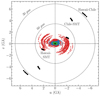 |
Fig. 1. (u, v)-coverage of 3C 84, as observed with the VLBA (15 GHz, green), VLBA (43 GHz, blue), GMVA (86 GHz, red), and EHT (228 GHz, black). Dashed circles indicate fringe spacings characterising the instrumental resolution of 60 μas and 30 μas. ‘Chile’ denotes stations ALMA and APEX. ‘Hawaii’ denotes stations SMA and JCMT. With the higher frequency observations and longer baselines of the EHT, we improve the angular resolution by a factor of > 2. |
For our analysis we assumed a BH mass of M• = 8 × 10⁸ M⊙ (Scharwächter et al. 2013), for which 100 μas corresponds to ∼500 Rs (∼800 Rs deprojected). We used H0 = 69.6 and ΩM = 0.286 in a flat cosmology (Bennett et al. 2014), yielding a length scale of ψ = 0.36 pc mas−1. Hence, 250 RS ≈ 54 μas ≈ 0.02 pc (0.032 pc de-projected) at z = 0.0176.
2.2. Results
We find evidence of a highly ordered, strong magnetic field in the submas compact region of 3C 84. This region is best fitted by three circular Gaussian components, labelled core (‘C’), east (‘E’), and west (‘W’), as shown in Fig. 2 (the method we used is described in Appendix B). The extended flux density detected on the short ALMA-APEX and JCMT-SMA baselines, while resolved out on all long EHT baselines, was fitted by a ∼5000 microarcseconds (μas) circular Gaussian component with a flux density of  . Furthermore, by averaging1 the linear fractional polarisation measurements of these three components, we determined the net linear fractional polarisation in the compact region to be mnet = (17.0 ± 3.9)%. The short baseline between ALMA and APEX yielded an estimate for the linear fractional polarisation on larger arcsecond scales, of ∼6% (denoted in the bottom panel of Fig. 3 with the grey marker).
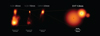 |
Fig. 2. Total intensity jet morphology of 3C 84 at different wavelengths. From left to right, we display the 15, 43, 86 (images), and 228 GHz (model) measurements. The horizontal line below each image represents the angular scale. The effective beam sizes, corresponding to these observations are, from left to right, 0.40 × 0.60 mas, 0.34 × 0.16 mas, 0.11 × 0.04 mas, and 107 × 14 μas. RS denotes the Schwarzschild radius. |
We cross-referenced the submas compact region model fit components at lower frequencies following the method detailed in Savolainen et al. (2008) and Appendix C. While at 15 GHz the submas region appears fully blended, we are able to recover the 228 GHz structure at 86 GHz and even at 43 GHz. The results are reported in Table A.1.
We also measured both the total intensity I and linearly polarised emission P in the submas region of 3C 84 in the 15, 43, and 86 GHz images. The values of linear fractional polarisation at these three lower frequencies are considered as upper limit estimates. The results are shown in Fig. 3. The VLBI total intensity increases up to the 86 GHz measurement, and then decreases towards 228 GHz.
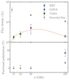 |
Fig. 3. VLBI and single-dish total intensity and fractional polarisation versus frequency for 3C 84, observed in March and April 2017. Top: green box markers, purple dot, and light blue diamond denote the total intensity, compact-scale VLBI flux density measurements at 15, 43, 86, and 228 GHz, respectively. The latter data point is the sum of components E, C, and W (see Table A.1). The orange line denotes the fit to the spectrum using Eq. (D.1). The grey star markers denote the single-dish (extended) flux density measurements at 8 (QUIVER), 86, and 228 GHz (POLAMI). The turnover frequency is between 86 and 228 GHz. The 8 GHz single-dish flux density is higher than at 86 GHz, because the parsec-scale jet flux density contributes to the measurement. Bottom: green and purple arrows indicate the upper limits of the fractional polarisation at 15, 43, and 86 GHz measured in the same region as the total intensity values in the upper panel. The light blue diamond marker again indicates the EHT measurement at 228 GHz. The grey star marker indicates the zero-baseline fractional polarisation on the baseline between ALMA and APEX. Error bars in both panels indicate the 68% confidence level. |
Close-in-time single-dish measurements at 8, 86, and 228 GHz are also shown in Fig. 3 (see also Table A.2). The 86 GHz flux density is higher than that at 228 GHz. However, the 8 GHz measurement is also higher than at 86 GHz, suggesting a significant contribution from the parsec-scale jet. Furthermore, at 228 GHz, the compact-scale VLBI flux density is significantly lower than the corresponding extended flux density, as long EHT baselines over-resolve the large-scale jet emission structure (similar to M 87, see e.g., The Event Horizon Telescope Collaboration 2019d). In terms of fractional polarisation, it is evident that there is a significant increase at 228 GHz, indicating a transition in the accretion flow to the optically thin regime.
3. Discussion
3.1. Insights from the synchrotron spectrum
Our analysis shows that the east–west elongated core structure (Giovannini et al. 2018) also persists at 1.3 mm, and in lower frequencies (as reported at 7 mm by Punsly et al. 2021 and 3 mm by Oh et al. 2022). Interpretation of the nature of the components comprising this broad core structure heavily depends on the uncertain jet viewing angle (ξ). An upper limit of ξ ∼ 40° was reported by Oh et al. (2022) based on a VLBI analysis of the compact region, but much lower values have also been found, for example based on γ-ray analysis (Abdo et al. 2009). The historically subluminal jet component velocities in the compact region (Punsly et al. 2021; Hodgson et al. 2021; Paraschos et al. 2022b) point towards an increased viewing angle. Moreover, different parts of the jet have been reported to be moving with different velocities, which is related to the so-called ‘Doppler crisis’ phenomenon (e.g., Henri & Saugé 2006) and jet stratification (Nagai et al. 2014).
The high-resolution, high-frequency EHT observation enables a novel diagnosis of the state of plasma surrounding the central black hole via calculation of the turnover frequency νm and the synchrotron self-absorption magnetic field strength BSSA. Assuming νm to be 86 GHz, Hodgson et al. (2018) and Kim et al. (2019) computed the BSSA to be ∼21 G. Using additional EHT flux density measurements, we can directly measure νm. While the different observations correspond to different (u, v) coverages, we fitted a focused Gaussian model to the high-signal-to-noise ratio (S/N) data at 228 GHz, finding core diameters within the order of magnitude of the diffraction limit. We also fixed the sizes of the components for all the frequencies in order to mitigate the effects of the different (u, v) coverages (see Table A.1). Subsequently, fitting, then, Eq. (5.90) from Condon & Ransom (2016) (see also Rybicki & Lightman 1979 and Appendix D) to the data yields νm = (113 ± 4) GHz (see also Türler et al. 2000). We computed a core brightness temperature of TB = (3.6 ± 1.5)×1011 K from νm, assuming that the angular size of the components at νm is the same as at 228 GHz (as the system is optically thin at both frequencies). Within the error budget, the system seems to be in equipartition (Singal 1986) between kinetic and magnetic energies (also reported by Paraschos et al. 2023, based on light-curve variability analysis).
Furthermore, we computed BSSA = (2.9 ± 1.6) G using Eq. (2) from Marscher (1983) (see also Appendix D). We also calculated an equipartition magnetic field strength of Beq = (5.2 ± 0.6) G. The uncertainties were calculated through standard error propagation. The two values agree with each other within the error budget. Our results also tentatively agree within the error budget with the magnetic field reported by Kim et al. (2019). The equipartition Doppler factor is δeq = 1.5 ± 0.4, suggesting that the acceleration happens further downstream, which is in line with lower frequency observations of 3C 84 (e.g., Hodgson et al. 2018; Paraschos et al. 2022b, and references therein).
Moreover, the equipartition magnetic field strength Beq in the vicinity of the jet apex was computed to reach up to 4 G in a core shift analysis carried out by Paraschos et al. (2021). However, the magnetic field value mentioned by these latter authors was calculated at the distance between the extrapolated jet apex and the 86 GHz core, resulting in a slightly lower estimate than that found in this work. Nevertheless, it is important to exercise caution when interpreting both νm and BSSA. 3C 84 is a variable source (recently up to 20–30% variation in total intensity and linear polarised flux density at 43 GHz within a year based on the monitoring program VLBA-BU-BLAZAR), which means that these observables might be time dependent (compare with the spectrum shown in, e.g., Hodgson et al. 2018). Moreover, our models still contain large uncertainties due to the sparsity of the (u, v) coverage, which may not be fully accounted for.
3.2. Model interpretation
Possible interpretations of the physical mechanisms driving the wide core structure largely depend on the exact location of the central engine with regard to the observed core. The current understanding is that the central engine is located north or northwest of the 86 GHz VLBI core (Giovannini et al. 2018; Paraschos et al. 2021). As its exact location is still ambiguous, it is unclear whether or not some of the identified components in this work correspond to the core (Case I) or a counter-jet (Case II).
Simulations of the radio jet of M 87 (Mościbrodzka et al. 2017) show that the linear polarisation is produced inside the approaching jet, while the dense accretion disc depolarises any radiation reaching us from the counter-jet. In 3C 84, circumnuclear free-free absorption has already been reported for example by Walker et al. (2000), who cite a possible connection to the accretion disc. It is thought that the presence of this disc obscures the counter-jet in the milliarcsecond (mas) region of 3C 84, which only becomes visible at a distance of > 2 mas at higher frequencies (as reported e.g., in Wajima et al. 2020 at 86 GHz). As both E and W in Fig. B.1 are highly linearly polarised (20–80%), this points towards Case I, meaning that the two components might be at the origin of the double-rail structure seen on larger scales, as opposed to a jet and counter-jet geometry. However, we note that this interpretation remains speculative, given the uncertainties.
This high fractional polarisation in E and W could be evidence for highly ordered magnetic field lines in the jet plasma with almost no Faraday depolarisation present. On the other hand, C has lower fractional polarisation and the synchrotron opacity should be nearly negligible at 228 GHz according to the Stokes I spectrum shown in Fig. 3. This may indicate that the main source of depolarisation in the compact region probed by the EHT is beam depolarisation of complex magnetic field patterns or mild Faraday depolarisation, rather than opacity effects. Consequently, a possible Faraday screen located in the compact region could be at most the size of C, which is ∼20 μas. However, it should be noted here that W is the most uncertain low-total-intensity component, hindering a reliable conclusion about its nature (see also Appendices A and B).
3C 84 is known to show high amounts of Faraday rotation (RM) and the presence of circular polarisation (see e.g., the POLAMI and QUIVER programmes as described in Agudo et al. 2018; Myserlis et al. 2018, respectively). Using the SMA and CARMA, Plambeck et al. (2014) reported an RM of as high as ∼ 9 × 10⁵ rad m−2, indicative of the presence of a strong magnetic field. This places 3C 84 in a small group of known radio sources exhibiting similarly high RMs, such as Sgr A* (∼ 5 × 10⁵ rad m−2; Wielgus et al. 2022 and references therein), M 87 (∼ 105 rad m−2; Goddi et al. 2021), and PKS 1830-211 (∼ 108 rad m−2; Martí-Vidal et al. 2015). However, whether this RM occurs in the medium surrounding the jet (e.g. from a disc wind) or is connected to the accretion flow remains unknown. The origin of the RM can be explored by determining its dependence on the observing frequency (Plambeck et al. 2014; Goddi et al. 2021) or the distance from the central engine (Park et al. 2015).
The density of the accretion flow, which is a related quantity that can be estimated via the RM, is required in order to constrain the mass-accretion rate around BHs (see Nagai et al. 2017, for a relevant discussion about 3C 84) for different accretion flow models, such as advection-dominated accretion flows (ADAFs; see Narayan & Yi 1995) and convection-dominated accretion flows (CDAFs; see Narayan et al. 2000).
Different plausible depolarisation mechanisms have been proposed for 3C 84, that is, originating from such an accretion flow and the jet itself (Li et al. 2016; Kim et al. 2019). Combining the single-dish data presented in Fig. 3, which were taken quasi-simultaneously with the EHT observations, allows us to estimate an estimate of the RM present in 3C 84. We find that RM = (6.06 ± 0.01)×106 rad m−2 by determining the gradient of the EVPAs as a function of the wavelength squared (see also Kim et al. 2019). The nπ ambiguity was resolved beforehand, as described in Hovatta et al. (2012). Such large RM values could be produced by the presence of relativistic and thermal electrons in the boundary layer between the jet and the interstellar medium, as reported in Goddi et al. (2021) for the jet in M 87.
3.3. Physical consequences
The high fractional linear polarisation in the innermost region of 3C 84, revealed at 228 GHz, clearly indicates that we are probing a previously elusive region, as we are able to achieve higher resolution while being less affected by opacity effects. We are probing the innermost region of 3C 84 at ∼500 Rs, which appears to be an optically thin region with an ordered magnetic field framing the core.
Furthermore, this region is so compact that an association between the broad jet of 3C 84 and the accretion disk can be ruled out. However, it should be pointed out that both a BH-driven jet and a disc-driven wind could coexist and the present EHT observations are a better probe of the former. In a BH-driven jet scenario, jet launching in 3C 84 might be attributed to a magnetically arrested disc (MAD; see similar simulations carried out for M 87 in Chael et al. 2019), as opposed to a thin, broad disc structure (Liska et al. 2019). Jets in MAD ADAF systems are likely launched by the Blandford–Znajek mechanism Blandford & Znajek (1977), which is the case where a powerful jet spine is powered directly by the energy extracted from the ergosphere of the BH.
Using our estimate of the RM at 228 GHz, it is possible to test whether the magnetic field reaches saturation strength; that is, whether the system is in the MAD state (Narayan et al. 2000; Tchekhovskoy et al. 2011). Under the assumptions described in Appendix E, we find that the dimensionless magnetic flux ϕ = 41 − 93 (Tchekhovskoy et al. 2011). Values above the saturation value ϕmax = 50 indicate that the jet is in a magnetically arrested state, and therefore our analysis suggests that jet launching in 3C 84 is MAD. As higher BH spin values and β = 1.5 produce values close to ϕmax, our result indicates a preference for a high BH spin and the ADAF model. 3C 84 is also classified as a low-luminosity AGN for which ADAF models are commonly invoked (de Menezes et al. 2020), further strengthening our conclusion. The mass-accretion rate estimated in Appendix E corresponds to Ṁ ∼ 10−5 − 10−4 ṀEdd, which is somewhat larger than in the case of M 87 MAD models (see e.g. The Event Horizon Telescope Collaboration 2021b). This suggests that a non-negligible dynamical impact of radiation is possible, which could challenge the applicability of the presented analysis. It should be pointed out here that it is unclear whether Faraday rotation takes place exclusively inside the accretion flow. Our analysis described in Appendix E is based on the assumption that the accretion flow is dominant.
If a spine-sheath geometry (Tavecchio & Ghisellini 2014) is present, manifested in the observations as a transverse velocity gradient, it could also be the underlying depolarising structure. In this case the rotation of the central BH leads to an inhomogeneous and twisted magnetic field topology (see for example Tchekhovskoy 2015). Furthermore, this scenario would also provide an explanation for the Doppler crisis. As discussed in Hodgson et al. (2021), so-called ‘jet-in-jet’ formations (Giannios et al. 2009) associated with velocity stratification in the bulk jet flow could be responsible for the enhanced γ-ray emission observed in 3C 84. Such a spine-sheath geometry has already been shown by the EHT to exist on small scales in the jet-launching region of Centaurus A (Janssen et al. 2021).
Ultimately, our detection of the exceptionally high fractional polarisation at 228 GHz, the peculiar jet morphology, and the detailed radio spectrum suggest that the jet in 3C 84 might be launched from both the central BH and the surrounding accretion disc (e.g., Blandford & Globus 2022). As shown by the present findings, millimetre VLBI observations pave the way towards probing the ultimate vicinity of BHs. Future 3C 84 EHT observations with added antennas on short and intermediate baselines will help to constrain the jet morphology and improve the fidelity of the model.
4. Conclusions
In this work we present the first detection of microarcsecond-scale polarised structures with the EHT. Our findings can be summarised as follows:
-
We report the first ever 228 GHz VLBI model of 3C 84, which reveals that the compact region is made up of three components.
-
We find a high degree of net fractional polarisation mnet = (17.0 ± 3.9)%. The brightness temperature is Tb = (3.6 ± 1.5)×1011 K, which suggests that the system is in equipartition.
-
Using quasi-simultaneous observations of 3C 84 at 15, 43, 86, and 228 GHz, we compute a turnover (optical depth τ = 1) frequency of νm = (113 ± 4) GHz, a synchrotron self-absorbed magnetic field of BSSA = (2.9 ± 1.6) G, and an equipartition magnetic field of Beq = (5.2 ± 0.6) G. However, these values might be influenced by the known variability of the source.
-
The increased values of linear polarisation suggest that the observed structure is the approaching jet, which is consistent with the large opening angle. Such a geometry can be produced by a thick disc associated with a Blandford & Znajek (1977) jet-launching scenario.
-
We find indications of a preference for higher values of BH spin and the ADAF model in the context of the MAD jet launching prevalent in 3C 84.
The EHT is an excellent instrument for probing AGN cores in nearby radio galaxies. Combined with lower frequency VLBI arrays, such as the GMVA and the VLBA, the EHT makes it possible to conduct multi-frequency studies, which provide valuable insights into jet formation and jet launching. New EHT and GMVA observations have already been carried out, with 3C 84 as the main target. The increased sensitivity and (u, v) coverage will enable us to conduct follow-up studies with higher fidelity. Total intensity images of the compact region will shed more light on whether or not the components we were able to identify here correspond to the broad structure seen with RadioAstron (Giovannini et al. 2018). Spectral index maps of EHT and GMVA images observed quasi-simultaneously might also assist in pinpointing the exact location of the BH (see e.g., Fig. 4 in Paraschos et al. 2022a) and in discriminating between jet launching-scenarios.
We used the formula 100%×|∑(Q + ιU)|/∑I, with I, Q, and U being the image domain Stokes parameters, and performed the pixel-wise summation over the whole field of view.
Here, we assume equipartition between cosmic-ray and magnetic energy density.
Acknowledgments
We thank the anonymous referee for the constructive suggestions which improved this manuscript. The Event Horizon Telescope Collaboration thanks the following organizations and programs: the Academia Sinica; the Academy of Finland (projects 274477, 284495, 312496, 315721); the Agencia Nacional de Investigación y Desarrollo (ANID), Chile via NCN19_058 (TITANs) and Fondecyt 1221421, the Alexander von Humboldt Stiftung; an Alfred P. Sloan Research Fellowship; Allegro, the European ALMA Regional Centre node in the Netherlands, the NL astronomy research network NOVA and the astronomy institutes of the University of Amsterdam, Leiden University, and Radboud University; the ALMA North America Development Fund; the Astrophysics and High Energy Physics programme by MCIN (with funding from European Union NextGenerationEU, PRTR-C17I1); the Black Hole Initiative, which is funded by grants from the John Templeton Foundation and the Gordon and Betty Moore Foundation (although the opinions expressed in this work are those of the author(s) and do not necessarily reflect the views of these Foundations); the Brinson Foundation; “la Caixa” Foundation (ID 100010434) through fellowship codes LCF/BQ/DI22/11940027 and LCF/BQ/DI22/11940030; Chandra DD7-18089X and TM6-17006X; the China Scholarship Council; the China Postdoctoral Science Foundation fellowships (2020M671266, 2022M712084); Consejo Nacional de Ciencia y Tecnología (CONACYT, Mexico, projects U0004-246083, U0004-259839, F0003-272050, M0037-279006, F0003-281692, 104497, 275201, 263356); the Consejería de Economía, Conocimiento, Empresas y Universidad of the Junta de Andalucía (grant P18-FR-1769), the Consejo Superior de Investigaciones Científicas (grant 2019AEP112); the Delaney Family via the Delaney Family John A. Wheeler Chair at Perimeter Institute; Dirección General de Asuntos del Personal Académico-Universidad Nacional Autónoma de México (DGAPA-UNAM, projects IN112417 and IN112820); the Dutch Organization for Scientific Research (NWO) for the VICI award (grant 639.043.513), the grant OCENW.KLEIN.113, and the Dutch Black Hole Consortium (with project No. NWA 1292.19.202) of the research programme the National Science Agenda; the Dutch National Supercomputers, Cartesius and Snellius (NWO grant 2021.013); the EACOA Fellowship awarded by the East Asia Core Observatories Association, which consists of the Academia Sinica Institute of Astronomy and Astrophysics, the National Astronomical Observatory of Japan, Center for Astronomical Mega-Science, Chinese Academy of Sciences, and the Korea Astronomy and Space Science Institute; the European Research Council (ERC) Synergy Grant “BlackHoleCam: Imaging the Event Horizon of Black Holes” (grant 610058); the European Union Horizon 2020 research and innovation programme under grant agreements RadioNet (No. 730562) and M2FINDERS (No. 101018682); the Horizon ERC Grants 2021 programme under grant agreement No. 101040021; the Generalitat Valenciana (grants APOSTD/2018/177 and ASFAE/2022/018) and GenT Program (project CIDEGENT/2018/021); MICINN Research Project PID2019-108995GB-C22; the European Research Council for advanced grant ‘JETSET: Launching, propagation and emission of relativistic jets from binary mergers and across mass scales’ (grant No. 884631); the FAPESP (Fundação de Amparo á Pesquisa do Estado de São Paulo) under grant 2021/01183-8; the Institute for Advanced Study; the Istituto Nazionale di Fisica Nucleare (INFN) sezione di Napoli, iniziative specifiche TEONGRAV; the International Max Planck Research School for Astronomy and Astrophysics at the Universities of Bonn and Cologne; DFG research grant “Jet physics on horizon scales and beyond” (grant No. FR 4069/2-1); Joint Columbia/Flatiron Postdoctoral Fellowship (research at the Flatiron Institute is supported by the Simons Foundation); the Japan Ministry of Education, Culture, Sports, Science and Technology (MEXT; grant JPMXP1020200109); the Japan Society for the Promotion of Science (JSPS) Grant-in-Aid for JSPS Research Fellowship (JP17J08829); the Joint Institute for Computational Fundamental Science, Japan; the Key Research Program of Frontier Sciences, Chinese Academy of Sciences (CAS, grants QYZDJ-SSW-SLH057, QYZDJSSW-SYS008, ZDBS-LY-SLH011); the Leverhulme Trust Early Career Research Fellowship; the Max-Planck-Gesellschaft (MPG); the Max Planck Partner Group of the MPG and the CAS; the MEXT/JSPS KAKENHI (grants 18KK0090, JP21H01137, JP18H03721, JP18K13594, 18K03709, JP19K14761, 18H01245, 25120007); the Malaysian Fundamental Research Grant Scheme (FRGS) FRGS/1/2019/STG02/UM/02/6; the MIT International Science and Technology Initiatives (MISTI) Funds; the Ministry of Science and Technology (MOST) of Taiwan (103-2119-M-001-010-MY2, 105-2112-M-001-025-MY3, 105-2119-M-001-042, 106-2112-M-001-011, 106-2119-M-001-013, 106-2119-M-001-027, 106-2923-M-001-005, 107-2119-M-001-017, 107-2119-M-001-020, 107-2119-M-001-041, 107-2119-M-110-005, 107-2923-M-001-009, 108-2112-M-001-048, 108-2112-M-001-051, 108-2923-M-001-002, 109-2112-M-001-025, 109-2124-M-001-005, 109-2923-M-001-001, 110-2112-M-003-007-MY2, 110-2112-M-001-033, 110-2124-M-001-007, and 110-2923-M-001-001); the Ministry of Education (MoE) of Taiwan Yushan Young Scholar Program; the Physics Division, National Center for Theoretical Sciences of Taiwan; the National Aeronautics and Space Administration (NASA, Fermi Guest Investigator grant 80NSSC20K1567, NASA Astrophysics Theory Program grant 80NSSC20K0527, NASA NuSTAR award 80NSSC20K0645); NASA Hubble Fellowship grants HST-HF2-51431.001-A, HST-HF2-51482.001-A awarded by the Space Telescope Science Institute, which is operated by the Association of Universities for Research in Astronomy, Inc., for NASA, under contract NAS5-26555; the National Institute of Natural Sciences (NINS) of Japan; the National Key Research and Development Program of China (grant 2016YFA0400704, 2017YFA0402703, 2016YFA0400702); the National Science Foundation (NSF, grants AST-0096454, AST-0352953, AST-0521233, AST-0705062, AST-0905844, AST-0922984, AST-1126433, AST-1140030, DGE-1144085, AST-1207704, AST-1207730, AST-1207752, MRI-1228509, OPP-1248097, AST-1310896, AST-1440254, AST-1555365, AST-1614868, AST-1615796, AST-1715061, AST-1716327, AST-1716536, OISE-1743747, AST-1816420, AST-1935980, AST-2034306); NSF Astronomy and Astrophysics Postdoctoral Fellowship (AST-1903847); the Natural Science Foundation of China (grants 11650110427, 10625314, 11721303, 11725312, 11873028, 11933007, 11991052, 11991053, 12192220, 12192223); the Natural Sciences and Engineering Research Council of Canada (NSERC, including a Discovery Grant and the NSERC Alexander Graham Bell Canada Graduate Scholarships-Doctoral Program); the National Youth Thousand Talents Program of China; the National Research Foundation of Korea (the Global PhD Fellowship Grant: grants NRF-2015H1A2A1033752, the Korea Research Fellowship Program: NRF-2015H1D3A1066561, Brain Pool Program: 2019H1D3A1A01102564, Basic Research Support Grant 2019R1F1A1059721, 2021R1A6A3A01086420, 2022R1C1C1005255); Netherlands Research School for Astronomy (NOVA) Virtual Institute of Accretion (VIA) postdoctoral fellowships; Onsala Space Observatory (OSO) national infrastructure, for the provisioning of its facilities/observational support (OSO receives funding through the Swedish Research Council under grant 2017-00648); the Perimeter Institute for Theoretical Physics (research at Perimeter Institute is supported by the Government of Canada through the Department of Innovation, Science and Economic Development and by the Province of Ontario through the Ministry of Research, Innovation and Science); the Princeton Gravity Initiative; the Spanish Ministerio de Ciencia e Innovación (grants PGC2018-098915-B-C21, AYA2016-80889-P, PID2019-108995GB-C21, PID2020-117404GB-C21); the University of Pretoria for financial aid in the provision of the new Cluster Server nodes and SuperMicro (USA) for a SEEDING GRANT approved toward these nodes in 2020; the Shanghai Pilot Program for Basic Research, Chinese Academy of Science, Shanghai Branch (JCYJ-SHFY-2021-013); the State Agency for Research of the Spanish MCIU through the “Center of Excellence Severo Ochoa” award for the Instituto de Astrofísica de Andalucía (SEV-2017- 0709); the Spanish Ministry for Science and Innovation grant CEX2021-001131-S funded by MCIN/AEI/10.13039/501100011033; the Spinoza Prize SPI 78-409; the South African Research Chairs Initiative, through the South African Radio Astronomy Observatory (SARAO, grant ID 77948), which is a facility of the National Research Foundation (NRF), an agency of the Department of Science and Innovation (DSI) of South Africa; the Toray Science Foundation; the Swedish Research Council (VR); the US Department of Energy (USDOE) through the Los Alamos National Laboratory (operated by Triad National Security, LLC, for the National Nuclear Security Administration of the USDOE, contract 89233218CNA000001); and the YCAA Prize Postdoctoral Fellowship. We thank the staff at the participating observatories, correlation centers, and institutions for their enthusiastic support. This paper makes use of the following ALMA data: ADS/JAO.ALMA#2016.1.01154.V. ALMA is a partnership of the European Southern Observatory (ESO; Europe, representing its member states), NSF, and National Institutes of Natural Sciences of Japan, together with National Research Council (Canada), Ministry of Science and Technology (MOST; Taiwan), Academia Sinica Institute of Astronomy and Astrophysics (ASIAA; Taiwan), and Korea Astronomy and Space Science Institute (KASI; Republic of Korea), in cooperation with the Republic of Chile. The Joint ALMA Observatory is operated by ESO, Associated Universities, Inc. (AUI)/NRAO, and the National Astronomical Observatory of Japan (NAOJ). The NRAO is a facility of the NSF operated under cooperative agreement by AUI. This research used resources of the Oak Ridge Leadership Computing Facility at the Oak Ridge National Laboratory, which is supported by the Office of Science of the U.S. Department of Energy under contract No. DE-AC05-00OR22725; the ASTROVIVES FEDER infrastructure, with project code IDIFEDER-2021-086; the computing cluster of Shanghai VLBI correlator supported by the Special Fund for Astronomy from the Ministry of Finance in China; We also thank the Center for Computational Astrophysics, National Astronomical Observatory of Japan. This work was supported by FAPESP (Fundacao de Amparo a Pesquisa do Estado de Sao Paulo) under grant 2021/01183-8. APEX is a collaboration between the Max-Planck-Institut für Radioastronomie (Germany), ESO, and the Onsala Space Observatory (Sweden). The SMA is a joint project between the SAO and ASIAA and is funded by the Smithsonian Institution and the Academia Sinica. The JCMT is operated by the East Asian Observatory on behalf of the NAOJ, ASIAA, and KASI, as well as the Ministry of Finance of China, Chinese Academy of Sciences, and the National Key Research and Development Program (No. 2017YFA0402700) of China and Natural Science Foundation of China grant 11873028. Additional funding support for the JCMT is provided by the Science and Technologies Facility Council (UK) and participating universities in the UK and Canada. The LMT is a project operated by the Instituto Nacional de Astrófisica, Óptica, y Electrónica (Mexico) and the University of Massachusetts at Amherst (USA). The IRAM 30-m telescope on Pico Veleta, Spain is operated by IRAM and supported by CNRS (Centre National de la Recherche Scientifique, France), MPG (Max-Planck-Gesellschaft, Germany), and IGN (Instituto Geográfico Nacional, Spain). The SMT is operated by the Arizona Radio Observatory, a part of the Steward Observatory of the University of Arizona, with financial support of operations from the State of Arizona and financial support for instrumentation development from the NSF. Support for SPT participation in the EHT is provided by the National Science Foundation through award OPP-1852617 to the University of Chicago. Partial support is also provided by the Kavli Institute of Cosmological Physics at the University of Chicago. The SPT hydrogen maser was provided on loan from the GLT, courtesy of ASIAA. This work used the Extreme Science and Engineering Discovery Environment (XSEDE), supported by NSF grant ACI-1548562, and CyVerse, supported by NSF grants DBI-0735191, DBI-1265383, and DBI-1743442. XSEDE Stampede2 resource at TACC was allocated through TG-AST170024 and TG-AST080026N. XSEDE JetStream resource at PTI and TACC was allocated through AST170028. This research is part of the Frontera computing project at the Texas Advanced Computing Center through the Frontera Large-Scale Community Partnerships allocation AST20023. Frontera is made possible by National Science Foundation award OAC-1818253. This research was done using services provided by the OSG Consortium (Pordes et al. 2007; Sfiligoi et al. 2009), which is supported by the National Science Foundation award Nos. 2030508 and 1836650. Additional work used ABACUS2.0, which is part of the eScience center at Southern Denmark University. Simulations were also performed on the SuperMUC cluster at the LRZ in Garching, on the LOEWE cluster in CSC in Frankfurt, on the HazelHen cluster at the HLRS in Stuttgart, and on the Pi2.0 and Siyuan Mark-I at Shanghai Jiao Tong University. The computer resources of the Finnish IT Center for Science (CSC) and the Finnish Computing Competence Infrastructure (FCCI) project are acknowledged. This research was enabled in part by support provided by Compute Ontario (http://computeontario.ca), Calcul Quebec (http://www.calculquebec.ca), and Compute Canada (http://www.computecanada.ca). The EHTC has received generous donations of FPGA chips from Xilinx Inc., under the Xilinx University Program. The EHTC has benefited from technology shared under open-source license by the Collaboration for Astronomy Signal Processing and Electronics Research (CASPER). The EHT project is grateful to T4Science and Microsemi for their assistance with hydrogen masers. This research has made use of NASA’s Astrophysics Data System. We gratefully acknowledge the support provided by the extended staff of the ALMA, from the inception of the ALMA Phasing Project through the observational campaigns of 2017 and 2018. Partly based on observations with the 100-m telescope of the MPIfR (Max-Planck-Institut für Radioastronomie) at Effelsberg. We would like to thank A. Deller and W. Brisken for EHT-specific support with the use of DiFX. We thank Jack Livingston for his comments. We acknowledge the significance that Maunakea, where the SMA and JCMT EHT stations are located, has for the indigenous Hawaiian people.
References
- Abdo, A. A., Ackermann, M., Ajello, M., et al. 2009, ApJ, 699, 31 [Google Scholar]
- Agudo, I., Thum, C., Molina, S. N., et al. 2018, MNRAS, 474, 1427 [NASA ADS] [CrossRef] [Google Scholar]
- Beck, R., & Krause, M. 2005, Astron. Nachr., 326, 414 [Google Scholar]
- Bell, A. R. 1978, MNRAS, 182, 443 [Google Scholar]
- Bennett, C. L., Larson, D., Weiland, J. L., & Hinshaw, G. 2014, ApJ, 794, 135 [Google Scholar]
- Biermann, P. L., & Strittmatter, P. A. 1987, ApJ, 322, 643 [Google Scholar]
- Blackburn, L., Chan, C.-K., Crew, G. B., et al. 2019, ApJ, 882, 23 [Google Scholar]
- Blandford, R., & Globus, N. 2022, MNRAS, 514, 5141 [NASA ADS] [CrossRef] [Google Scholar]
- Blandford, R. D., & Payne, D. G. 1982, MNRAS, 199, 883 [CrossRef] [Google Scholar]
- Blandford, R. D., & Znajek, R. L. 1977, MNRAS, 179, 433 [NASA ADS] [CrossRef] [Google Scholar]
- Chael, A. A., Johnson, M. D., Narayan, R., et al. 2016, ApJ, 829, 11 [Google Scholar]
- Chael, A., Narayan, R., & Johnson, M. D. 2019, MNRAS, 486, 2873 [NASA ADS] [CrossRef] [Google Scholar]
- Chamani, W., Savolainen, T., Hada, K., & Xu, M. H. 2021, A&A, 652, A14 [NASA ADS] [CrossRef] [EDP Sciences] [Google Scholar]
- Condon, J. J., & Ransom, S. M. 2016, Essential Radio Astronomy (Princeton: Princeton University Press) [Google Scholar]
- de Menezes, R., Nemmen, R., Finke, J. D., Almeida, I., & Rani, B. 2020, MNRAS, 492, 4120 [NASA ADS] [CrossRef] [Google Scholar]
- Gardner, F. F., & Whiteoak, J. B. 1966, ARA&A, 4, 245 [NASA ADS] [CrossRef] [Google Scholar]
- Giannios, D., Uzdensky, D. A., & Begelman, M. C. 2009, MNRAS, 395, L29 [NASA ADS] [CrossRef] [Google Scholar]
- Giovannini, G., Savolainen, T., Orienti, M., et al. 2018, Nat. Astron., 2, 472 [Google Scholar]
- Goddi, C., Martí-Vidal, I., Messias, H., et al. 2019, PASP, 131, 075003 [Google Scholar]
- Goddi, C., Martí-Vidal, I., Messias, H., et al. 2021, ApJ, 910, L14 [NASA ADS] [CrossRef] [Google Scholar]
- Henri, G., & Saugé, L. 2006, ApJ, 640, 185 [NASA ADS] [CrossRef] [Google Scholar]
- Hodgson, J. A., Rani, B., Lee, S.-S., et al. 2018, MNRAS, 475, 368 [NASA ADS] [CrossRef] [Google Scholar]
- Hodgson, J. A., Rani, B., Oh, J., et al. 2021, ApJ, 914, 43 [NASA ADS] [CrossRef] [Google Scholar]
- Hovatta, T., Lister, M. L., Aller, M. F., et al. 2012, AJ, 144, 105 [Google Scholar]
- Issaoun, S., Wielgus, M., Jorstad, S., et al. 2022, ApJ, 934, 145 [NASA ADS] [CrossRef] [Google Scholar]
- Janssen, M., Goddi, C., van Bemmel, I. M., et al. 2019, A&A, 626, A75 [NASA ADS] [CrossRef] [EDP Sciences] [Google Scholar]
- Janssen, M., Falcke, H., Kadler, M., et al. 2021, Nat. Astron., 5, 1017 [NASA ADS] [CrossRef] [Google Scholar]
- Jorstad, S. G., Marscher, A. P., Morozova, D. A., et al. 2017, ApJ, 846, 98 [Google Scholar]
- Jorstad, S., Wielgus, M., Lico, R., et al. 2023, ApJ, 943, 170 [NASA ADS] [CrossRef] [Google Scholar]
- Kim, J. Y., Krichbaum, T. P., Lu, R. S., et al. 2018, A&A, 616, A188 [NASA ADS] [CrossRef] [EDP Sciences] [Google Scholar]
- Kim, J. Y., Krichbaum, T. P., Marscher, A. P., et al. 2019, A&A, 622, A196 [NASA ADS] [CrossRef] [EDP Sciences] [Google Scholar]
- Kovalev, Y. Y., Lobanov, A. P., Pushkarev, A. B., & Zensus, J. A. 2008, A&A, 483, 759 [NASA ADS] [CrossRef] [EDP Sciences] [Google Scholar]
- Kraus, A., Krichbaum, T. P., Wegner, R., et al. 2003, A&A, 401, 161 [NASA ADS] [CrossRef] [EDP Sciences] [Google Scholar]
- Li, Y.-P., Yuan, F., & Xie, F.-G. 2016, ApJ, 830, 78 [NASA ADS] [CrossRef] [Google Scholar]
- Liska, M., Tchekhovskoy, A., Ingram, A., & van der Klis, M. 2019, MNRAS, 487, 550 [CrossRef] [Google Scholar]
- Lister, M. L., Aller, M. F., Aller, H. D., et al. 2018, ApJS, 234, 12 [CrossRef] [Google Scholar]
- Marrone, D. P., Moran, J. M., Zhao, J.-H., & Rao, R. 2006, ApJ, 640, 308 [NASA ADS] [CrossRef] [Google Scholar]
- Marscher, A. P. 1983, ApJ, 264, 296 [Google Scholar]
- Martí-Vidal, I., Krichbaum, T. P., Marscher, A., et al. 2012, A&A, 542, A107 [NASA ADS] [CrossRef] [EDP Sciences] [Google Scholar]
- Martí-Vidal, I., Muller, S., Vlemmings, W., Horellou, C., & Aalto, S. 2015, Science, 348, 311 [Google Scholar]
- Martí-Vidal, I., Mus, A., Janssen, M., de Vicente, P., & González, J. 2021, A&A, 646, A52 [NASA ADS] [CrossRef] [EDP Sciences] [Google Scholar]
- Mościbrodzka, M., Dexter, J., Davelaar, J., & Falcke, H. 2017, MNRAS, 468, 2214 [CrossRef] [Google Scholar]
- Myserlis, I., Angelakis, E., Kraus, A., et al. 2018, A&A, 609, A68 [NASA ADS] [CrossRef] [EDP Sciences] [Google Scholar]
- Nagai, H., Haga, T., Giovannini, G., et al. 2014, ApJ, 785, 53 [Google Scholar]
- Nagai, H., Fujita, Y., Nakamura, M., et al. 2017, ApJ, 849, 52 [NASA ADS] [CrossRef] [Google Scholar]
- Narayan, R., & Yi, I. 1995, ApJ, 452, 710 [NASA ADS] [CrossRef] [Google Scholar]
- Narayan, R., Igumenshchev, I. V., & Abramowicz, M. A. 2000, ApJ, 539, 798 [NASA ADS] [CrossRef] [Google Scholar]
- Oh, J., Hodgson, J. A., Trippe, S., et al. 2022, MNRAS, 509, 1024 [Google Scholar]
- Pacholczyk, A. G. 1970, Radio Astrophysics. Nonthermal Processes in Galactic and Extragalactic Sources (San Francisco: Freeman) [Google Scholar]
- Paraschos, G. F., Kim, J. Y., Krichbaum, T. P., & Zensus, J. A. 2021, A&A, 650, L18 [NASA ADS] [CrossRef] [EDP Sciences] [Google Scholar]
- Paraschos, G., Kim, J. Y., Krichbaum, T., et al. 2022a, European VLBI Network Mini-Symposium and Users’ Meeting, 2021, 43 [Google Scholar]
- Paraschos, G. F., Krichbaum, T. P., Kim, J. Y., et al. 2022b, A&A, 665, A1 [NASA ADS] [CrossRef] [EDP Sciences] [Google Scholar]
- Paraschos, G. F., Mpisketzis, V., Kim, J. Y., et al. 2023, A&A, 669, A32 [NASA ADS] [CrossRef] [EDP Sciences] [Google Scholar]
- Park, J. H., Trippe, S., Krichbaum, T. P., et al. 2015, A&A, 576, L16 [NASA ADS] [CrossRef] [EDP Sciences] [Google Scholar]
- Plambeck, R. L., Bower, G. C., Rao, R., et al. 2014, ApJ, 797, 66 [NASA ADS] [CrossRef] [Google Scholar]
- Pordes, R., Petravick, D., Kramer, B., et al. 2007, J. Phys. Conf. Ser., 78, 012057P [NASA ADS] [CrossRef] [Google Scholar]
- Punsly, B., Nagai, H., Savolainen, T., & Orienti, M. 2021, ApJ, 911, 19 [Google Scholar]
- Rafferty, D. A., McNamara, B. R., Nulsen, P. E. J., & Wise, M. W. 2006, ApJ, 652, 216 [NASA ADS] [CrossRef] [Google Scholar]
- Rybicki, G. B., & Lightman, A. P. 1979, Radiative Processes in Astrophysics (New York: Wiley) [Google Scholar]
- Savolainen, T., Wiik, K., Valtaoja, E., & Tornikoski, M. 2008, in Extragalactic Jets: Theory and Observation from Radio to Gamma Ray, eds. T. A. Rector, & D. S. De Young, ASP Conf. Ser., 386, 451 [NASA ADS] [Google Scholar]
- Scharwächter, J., McGregor, P. J., Dopita, M. A., & Beck, T. L. 2013, MNRAS, 429, 2315 [Google Scholar]
- Sfiligoi, I., Bradley, D. C., Holzman, B., et al. 2009, WRI World Congress on Computer Science and Information Engineering, 2, 428 [Google Scholar]
- Shepherd, M. C., Pearson, T. J., & Taylor, G. B. 1994, Bull. Am. Astron. Soc., 26, 987 [Google Scholar]
- Shepherd, M. C., Pearson, T. J., & Taylor, G. B. 1995, Bull. Am. Astron. Soc., 27, 903 [Google Scholar]
- Singal, A. K. 1986, A&A, 155, 242 [NASA ADS] [Google Scholar]
- Strauss, M. A., Huchra, J. P., Davis, M., et al. 1992, ApJS, 83, 29 [Google Scholar]
- Tavecchio, F., & Ghisellini, G. 2014, MNRAS, 443, 1224 [Google Scholar]
- Tchekhovskoy, A. 2015, in The Formation and Disruption of Black Hole Jets, eds. I. Contopoulos, D. Gabuzda, & N. Kylafis, Astrophys. Space Sci. Lib., 414, 45 [NASA ADS] [Google Scholar]
- Tchekhovskoy, A., Narayan, R., & McKinney, J. C. 2010, ApJ, 711, 50 [NASA ADS] [CrossRef] [Google Scholar]
- Tchekhovskoy, A., Narayan, R., & McKinney, J. C. 2011, MNRAS, 418, L79 [NASA ADS] [CrossRef] [Google Scholar]
- The Event Horizon Telescope Collaboration (Akiyama, K., et al.) 2019a, ApJ, 875, L1 [Google Scholar]
- The Event Horizon Telescope Collaboration (Akiyama, K., et al.) 2019b, ApJ, 875, L2 [Google Scholar]
- The Event Horizon Telescope Collaboration (Akiyama, K., et al.) 2019c, ApJ, 875, L3 [Google Scholar]
- The Event Horizon Telescope Collaboration (Akiyama, K., et al.) 2019d, ApJ, 875, L4 [Google Scholar]
- The Event Horizon Telescope Collaboration (Akiyama, K., et al.) 2021a, ApJ, 910, L12 [Google Scholar]
- The Event Horizon Telescope Collaboration (Akiyama, K., et al.) 2021b, ApJ, 910, L13 [Google Scholar]
- The Event Horizon Telescope Collaboration (Akiyama, K., et al.) 2022a, ApJ, 930, L12 [NASA ADS] [CrossRef] [Google Scholar]
- The Event Horizon Telescope Collaboration (Akiyama, K., et al.) 2022b, ApJ, 930, L13 [NASA ADS] [CrossRef] [Google Scholar]
- Thompson, A. R., Moran, J. M., Swenson, George W. J., 2017, Interferometry and Synthesis in Radio Astronomy, 3rd edn. (New York: Springer) [CrossRef] [Google Scholar]
- Thum, C., Wiesemeyer, H., Paubert, G., Navarro, S., & Morris, D. 2008, PASP, 120, 777 [NASA ADS] [CrossRef] [Google Scholar]
- Türler, M., Courvoisier, T. J. L., & Paltani, S. 2000, A&A, 361, 850 [Google Scholar]
- Virtanen, P., Gommers, R., Oliphant, T. E., et al. 2020, Nat. Methods, 17, 261 [Google Scholar]
- Wajima, K., Kino, M., & Kawakatu, N. 2020, ApJ, 895, 35 [Google Scholar]
- Walker, R. C., Dhawan, V., Romney, J. D., Kellermann, K. I., & Vermeulen, R. C. 2000, ApJ, 530, 233 [Google Scholar]
- Wielgus, M., Moscibrodzka, M., Vos, J., et al. 2022, A&A, 665, L6 [NASA ADS] [CrossRef] [EDP Sciences] [Google Scholar]
- Zamaninasab, M., Clausen-Brown, E., Savolainen, T., & Tchekhovskoy, A. 2014, Nature, 510, 126 [Google Scholar]
Appendix A: Additional methodology comments
The frequency setup of the EHT in 2017 consisted of two bands, each of 2 GHz in width, centred at 227.1 GHz (LO band) and 229.1 GHz (HI band): see The Event Horizon Telescope Collaboration (2019b) for details. For all the presented analyses, we combined data sets from both bands, using data points averaged over 2 GHz in frequency and for 120 s in time. In the EHT data sets, the polarimetric calibration relies on the calibration of ALMA (Goddi et al. 2019), which provides the absolute EVPA and serves as a reference site for the computation of the complex polarimetric gains for the entire EHT array (The Event Horizon Telescope Collaboration 2021a). As ALMA was present in only one-sixth of the observing scans of 3C 84, we only obtained the ALMA-based calibration for the single scan. The corresponding EVPA measurement on the short ALMA-APEX baseline is close to the north–south axis, consistent with POLAMI observations. This is in contrast to previous polarimetric analyses with the EHT (The Event Horizon Telescope Collaboration 2021a; Issaoun et al. 2022; Jorstad et al. 2023), where the absolute EVPA reference was always constrained by ALMA. As a consequence, the absolute EVPA calibration was found to be challenging and dependent on additional assumptions for the remaining part of the observations, with the additional difficulties related to APEX drop-outs in the HI band and JCMT observing only the right-hand circular polarisation component, which was used as as proxy for the total intensity in a similar way to in the previous EHT analyses (e.g. The Event Horizon Telescope Collaboration 2019a, 2022a). Hence, in the fitting to the linearly polarised source structure, we made a choice to only fit the absolute values of the fractional Fourier polarisation (corresponding to  , the amplitude ratio of cross-hand and parallel-hand visibility components, following the notation of The Event Horizon Telescope Collaboration 2021a), as shown in the right panel of Fig. A.1. We therefore neglect the corrupted linear polarisation phase information. As a consequence, we only interpret the absolute values of fractional polarisation of the fitted Gaussian components. In astrophysical synchrotron plasma, the following order of Stokes parameters magnitude is generally expected: I > |P|≫V; circular polarisation V is consequently neglected in the studies of total intensity I and linear polarisation P. Under this assumption, we can use single-polarisation JCMT data in the fitting to absolute values of Fourier fractional linear polarisation.
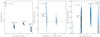 |
Fig. A.1. Best-fit model of 3C 84 compared to the data. Presented here from left to right are the data points (denoted with round blue markers) and models (denoted with dark orange crosses) of the visibility amplitudes, closure phases, and fractional polarisation as a function of the (u, v) distance. The combined (u, v) distance used in the middle panel is defined as the square root of the sum of squared lengths of all three baselines forming a triangle. Error bars in all panels indicate the 68% confidence level. |
The high quality of the fit is quantified with the reduced χ2, which is provided in Fig. A.1 for different data products used for the simultaneous fitting: visibility amplitudes, closure phases, and fractional Fourier linear polarisation (see e.g. The Event Horizon Telescope Collaboration 2021a, for the exact definition). Additionally, in Fig. A.2, the closure phases observed on the APEX-SMT-JCMT triangle are compared with our model (model 3g, with three Gaussian components representing the compact region emission). Non-zero closure phases are an immediate indication of a resolved structure, inconsistent with a circular symmetry of the source (Thompson et al. 2017).
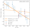 |
Fig. A.2. Closure phases as a function of the time of observation, detected on the APEX-SMT-JCMT non-trivial triangle, compared with the predictions of the model presented in this paper. Error bars indicate the 68% confidence level. The best-fit model 2g with two Gaussian components representing the compact emission region fails to adequately capture the trend in the data, unlike the 3g model with three components. The reported χ2 corresponds to the non-trivial subset of all measured closure phases. |
The dominant systematic uncertainty in the linear polarisation analysis results comes from the lack of the polarimetric leakage calibration (D-terms calibration; The Event Horizon Telescope Collaboration 2021a), which could not be directly employed for the 3C 84 data set, given the aforementioned data set issues pertaining to the uncertain, time-dependent EVPA calibration. In order to obtain a rough characterisation of the impact of the leakage on the resulting polarimetric quantities, we performed a small survey of data sets calibrated with different D-terms. We assumed the magnitude of the complex EHT array D-terms estimated and verified in previous EHT publications (The Event Horizon Telescope Collaboration 2021a; Issaoun et al. 2022; Jorstad et al. 2023), but generated ten random realisations of D-term phases, subsequently refitting the polarimetric source model to data sets with different leakage calibration variants. The fractional polarisation uncertainties reported in Table A.1 reflect the results of the D-term calibration survey.
Summary of the image parameters
Extended flux measurements
Appendix B: Modelling the EHT data
We modelled the EHT data with circular Gaussian components, because the (u, v) coverage is too sparse to reconstruct an image from it. Circular instead of elliptical Gaussian components were preferred in order to reduce the number of degrees of freedom. We used the forward modelling eht-imaging software (Chael et al. 2016) and leveraged heuristic optimisation tools implemented in SciPy (Virtanen et al. 2020) to search for the best-fit solution in terms of a minimum of an error function. Figure A.1 presents our best-fit model to the visibility amplitudes, closure phases, and fractional polarisation as a function of the (u, v) distance. Figure B.1 shows the fractional polarisation of the best-fit solution. See Appendix A for additional comments on the fitting procedure.
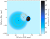 |
Fig. B.1. Fractional polarisation image. Shown here is a representation of the best-fit model to the fractional polarisation data in the image plane. Contours correspond to 0.5, 1, 5, 50, and 90% of the peak brightness temperature Tb = 3.6 × 10¹¹ K. We note the high net fractional linear polarisation of mnet = (17.0 ± 3.9)% in the compact region probed by the EHT. |
A certain degree of ambiguity in the compact source structure and the number of components is expected due to the large asymmetry of the EHT (u, v) coverage, which provides resolving power primarily along the south–east/north–west axis; see Fig. 1. In particular, we considered the choice between a two-component (2g) and a three-component (3g) model of the compact emission. The former corresponds to ten geometric degrees of freedom (i.e., not counting the amplitude gains) for the compact emission and three for the extended emission. The latter adds six degrees of freedom to the compact emission part. While in the data set used for fitting there are 86 visibility amplitudes, 14 non-trivial closure phases (all shown in Fig. A.2), and 80 absolute values of fractional linear polarisations, there are strong correlations between data points in time, frequency, and location on the (u, v) plane. The presence of such correlations reduces the effective constraining power of the data set. Hence, the model selection becomes a non-trivial problem. The best-fit 2g model essentially recovers the presented geometry of E and C components with the same fractional polarisation of C and around 35% polarisation of E. While the 2g model fits the amplitudes and fractional polarisations well, it is not capable of reproducing the closure phase measurements in a joint fit to all data products, which we demonstrate in Fig. A.2. This, along with earlier results obtained at lower observing frequencies (Punsly et al. 2021), motivates the selection of the 3g model for the presented analysis, despite it being slightly over-fitted according to the χ2 values reported in Fig. A.1. Such behaviour is generally expected for an accurate model given the strong correlations present in the data.
Appendix C: Multi-frequency template matching
We used circular Gaussian components to model the EHT data, determining the number of degrees of freedom required to accurately fit visibility amplitudes, closure phases, and fractional Fourier polarisation, including the modelling of station-based, time-dependent amplitude gains. This is made possible by using the template-matching technique (e.g. Savolainen et al. 2008; Kovalev et al. 2008), which leverages prior knowledge of the source’s brightness distribution from high-frequency measurements (here 228 GHz) to estimate the source structure at lower frequencies, even if they are closer together than the lower frequency beam size. Given sufficient S/N, structures smaller than the diffraction-limited interferometric resolution can be constrained (e.g. Martí-Vidal et al. 2012). For our observations, S/N ∼ 550 at 43 GHz and S/N ∼ 375 at 86 GHz, resulting in nominal resolution limits  and
and  , respectively. Therefore, we were able to apply the high-frequency template, given that the separation between the components comprising the template was sufficiently large. It should be noted here, that these calculations are performed under the assumption that the source’s morphology is a Gaussian. However, given the complex structure in the compact region of 3C 84 revealed here, the actual resolution may be worse. We therefore adopted the more conservative approach of restricting the resolution limit to the typical value of approximately one-fifth of the beam size (e.g. Oh et al. 2022). This was still possible in our case at 43 GHz (beam size ∼100 μas) and 86 GHz (beam size ∼50 μas). As in our work we investigate the overall spectral behaviour of the submas region, this approach is sufficient to get an estimate for the flux densities and fractional polarisations for each component. We also disregarded the core shift effects (see e.g. Paraschos et al. 2021; Oh et al. 2022; Paraschos et al. 2023) between the images at different frequencies, because their effect is negligible for our analysis (of the order of a few tens of μas). Our results are summarised in Table A.1. The uncertainties of the flux density measurements are on the order of 20% at 15 GHz, 30% at 43 GHz, 50% at 86 GHz, and 15% at 228 GHz (The Event Horizon Telescope Collaboration 2019c).
Appendix D: Magnetic field estimate
We estimated the magnetic field strength in the core via synchrotron turnover frequency fitting. The synchrotron spectrum takes the following form (Condon & Ransom 2016):
![Mathematical equation: $$ \begin{aligned} S(\nu ) = S_0 \left( \frac{\nu }{\nu _\text{1}} \right)^{\alpha _\text{thick}} \left\{ 1-\exp \left[ - \left( \frac{\nu }{\nu _\text{1}} \right)^{-(p+4)/2} \right] \right\} , \end{aligned} $$](/articles/aa/full_html/2024/02/aa48308-23/aa48308-23-eq5.gif) (D.1)
(D.1)
for a homogeneous and cylindrical source, where ν1 is the frequency where the opacity reaches unity, τ = 1, and S0 = 5.7 ± 0.3 Jy is a multiplication constant, determined from the fit. Subsequently, νm is calculated by determining the peak of the fitted spectrum. Following Kim et al. (2019), we set αthick = 0.51 ± 0.10. The parameter p is the power-law slope of the electron energy distribution function and is set to p = 2 (Condon & Ransom 2016).
We used two different prescriptions for the magnetic field strength. First we calculated the equipartition magnetic field Beq using Pacholczyk (1970) with the following form2:
![Mathematical equation: $$ \begin{aligned} \left(\frac{B_\text{eq}}{{\text{ G}}}\right)&= 2.7\times 10^{-7}\nonumber \\&\left[ \frac{\left(1+k_\text{u}\right)c_{12}\kappa _\nu }{f} \frac{S_\text{m}/\text{ Jy}}{(\theta /\text{ mas})^3}\frac{\nu _\text{m}/\text{ Hz}}{D_\text{L}/\text{ Gpc}} \frac{\left(1+z\right)^{10}}{\delta ^4} \right]^{2/7} . \end{aligned} $$](/articles/aa/full_html/2024/02/aa48308-23/aa48308-23-eq6.gif) (D.2)
(D.2)
We note that the exponent 2/7 only holds for αthin = 0.5 (see Beck & Krause 2005, for a relevant discussion). Here, ku is a ratio that provides an estimate of the energy in relativistic protons compared to electrons and f is a factor denoting the fraction of the total volume of the emitting region occupied by the plasma and magnetic field in equipartition. Under the assumption of an electron-positron pair plasma (see Paraschos et al. 2023, for a discussion about electron-positron pair plasma in the vicinity of the SMBH in 3C 84), which is volume filling, ku = 0 and f = 1. The uncertainties for ku and f are difficult to constrain; their impact on the magnetic field strength computation is discussed below. The constant c12 (in cgs units) is given by the following expression:
 (D.3)
(D.3)
where ![Mathematical equation: $ c_1 = \frac{3e}{4\pi m^3_\text{e}c^5} = 6.27\times10^{18}\,\text{[cgs]} $](/articles/aa/full_html/2024/02/aa48308-23/aa48308-23-eq8.gif) and
and ![Mathematical equation: $ c_2 = \frac{2e^4}{3 m^4_\text{e}c^7} = 2.37\times10^{-3}\,\text{[cgs]} $](/articles/aa/full_html/2024/02/aa48308-23/aa48308-23-eq9.gif) ; e and me are the charge and mass of the electron respectively and c is the speed of light. Furthermore, κν is defined as
; e and me are the charge and mass of the electron respectively and c is the speed of light. Furthermore, κν is defined as
 (D.4)
(D.4)
where νmin and νmax are the minimum and maximum frequency range of synchrotron radiation. We used νmin = 107 Hz (lowest possible frequency for synchrotron emission) and νmax = 3 × 10¹⁴ Hz (Biermann & Strittmatter 1987). As [νmin, νmax] constitute an assumed frequency range, their values are presented without uncertainties. The optically thin spectral index is αthin = −0.5 (Kim et al. 2019). The angular diameter is denoted as θ and the synchrotron peak flux density as Sm = 9.0 ± 0.5 Jy at the frequency νm, extrapolated from the optically thin flux density (see also Chamani et al. 2021). We assumed δ = 1.1 ± 0.1 for the Doppler factor based on observations presented in Kim et al. (2019), Punsly et al. (2021), Paraschos et al. (2021) and used θ = (144 ± 18) μas (this value already includes the geometric correction discussed in Marscher (1983)).
Additionally, using Eq. 2 in Marscher (1983):
 (D.5)
(D.5)
Our choice of αthin = −0.5 results in b(αthin) = 3.2. The resulting estimates for the magnetic field are BSSA = (2.9 ± 1.6) G and Beq = (5.2 ± 0.6) G for the core component C at 228 GHz. We point out that the BSSA calculation is strongly impacted by the value of νm. An increase or decrease of a few GHz would vary the value of BSSA by two orders of magnitude. Similarly, the Beq calculation strongly depends on the assumption of ku, that is, the particle composition of the jet. Alternative assumptions of the jet composition resulting in an increase in ku (diffusive shock acceleration would result in values of ku ≤ 50, see e.g. Bell 1978) would increase the value of Beq by up to a factor of 3. Likewise, decreasing the value of f (assuming a clumpier medium, filling only half of the total emitting region for example), would result in an increase in Beq by a factor of 1.2. However, we note that the good agreement between the two magnetic field estimates indicates that the choice of ku = 0 and f = 1 is reasonable. The equipartition Doppler factor required for BSSA to match Beq is δeq = 1.5 ± 0.4.
Finally, we can compare Beq and BSSA to the strength of the coherent field based on the observed RM. Using Eq. 15 from Gardner & Whiteoak (1966), written:
 (D.6)
(D.6)
we can compute the lower limit of the strength of the ordered field,  . Here, ne is the number density of the thermal electrons, which we set to ne = 3 × 104 cm−3 (Scharwächter et al. 2013). The path length of integration through the plasma is dl and can be approximated by ψ × θ. Using these values,
  , which is consistent as a lower limit to our calculations of Beq and BSSA.
Appendix E: Dimensionless magnetic flux
We calculated the dimensionless magnetic flux ϕ using the expression for the jet power Pjet Tchekhovskoy et al. (2010), which holds for black hole spin values α* ≤ 1:
![Mathematical equation: $$ \begin{aligned} \left(\frac{P_\text{jet}}{\dot{M}\text{ c}^2}\right) = \frac{\kappa }{4\pi }\phi ^2\Omega _\text{H}^2\left[1+1.38\Omega _\text{H}^2-9.2\Omega _\text{H}^4\right]. \end{aligned} $$](/articles/aa/full_html/2024/02/aa48308-23/aa48308-23-eq15.gif) (E.1)
(E.1)
Here,  , Ṁ is the mass-accretion rate of 3C 84, and κ = 0.05 is a constant depending on the initial field geometry.
To determine the mass-accretion rate, we use Eq. 9 from Marrone et al. (2006), in the following form (as also shown in Nagai et al. 2017):
 (E.2)
(E.2)
where β = 0.5 for CDAF or β = 1.5 for ADAF and rin and rout are the inner and outer effective radii of the accretion flow. Furthermore, ṀEdd = LEdd/(ϵc2), where ϵ is an efficiency factor. Using LEdd ∼ 1047 erg s−1 (Plambeck et al. 2014), ϵ = 0.1, rout ∼ 105 Rs (Nagai et al. 2017), rin ∼ 90 Rs (size of C), and RM = (6.06 ± 0.01)×106 rad m−2 yields Ṁ = 0.3 × 10⁻³ M⊙ yr−1 for β = 0.5 and Ṁ ∼ 1.1 × 10⁻³ M⊙ yr−1 β = 1.5. This computation rests on the assumption that the Faraday screen is external. Our assumption is physically motivated; the jet viewing angle used in our computations (ξ ∼ 40°) is larger than half of the intrinsic jet opening angle (i ≲ 20°; see e.g. Paraschos et al. 2021), suggesting that we are peering through the jet sheath and boundary layer (see also Plambeck et al. 2014; Nagai et al. 2017). Furthermore, at 1.3 mm, we are able to directly examine the environment of the central engine, because the opacity effects become comparatively minor.
Finally, the total luminosity of the jet in 3C 84 (Rafferty et al. 2006) is Pjet = 1.5 × 1044 erg s−1. Thus, setting a* = 1, we computed a range of ϕ = 41 − 93. Values of ϕ ≳ 50 refer to MAD models (Tchekhovskoy et al. 2011; Zamaninasab et al. 2014). We note here that the RM would need to be underestimated by more than an order of magnitude (e.g. due to the Faraday screen not being external) for ϕ to equal its MAD saturation value. Our investigation of different flow geometries and black hole spins supports an advection-dominated accretion flow in a magnetically arrested state as a model of the jet launching system in the core of 3C 84.
All Tables
All Figures
|
Fig. 1. (u, v)-coverage of 3C 84, as observed with the VLBA (15 GHz, green), VLBA (43 GHz, blue), GMVA (86 GHz, red), and EHT (228 GHz, black). Dashed circles indicate fringe spacings characterising the instrumental resolution of 60 μas and 30 μas. ‘Chile’ denotes stations ALMA and APEX. ‘Hawaii’ denotes stations SMA and JCMT. With the higher frequency observations and longer baselines of the EHT, we improve the angular resolution by a factor of > 2. |
| In the text | |
|
Fig. 2. Total intensity jet morphology of 3C 84 at different wavelengths. From left to right, we display the 15, 43, 86 (images), and 228 GHz (model) measurements. The horizontal line below each image represents the angular scale. The effective beam sizes, corresponding to these observations are, from left to right, 0.40 × 0.60 mas, 0.34 × 0.16 mas, 0.11 × 0.04 mas, and 107 × 14 μas. RS denotes the Schwarzschild radius. |
| In the text | |
|
Fig. 3. VLBI and single-dish total intensity and fractional polarisation versus frequency for 3C 84, observed in March and April 2017. Top: green box markers, purple dot, and light blue diamond denote the total intensity, compact-scale VLBI flux density measurements at 15, 43, 86, and 228 GHz, respectively. The latter data point is the sum of components E, C, and W (see Table A.1). The orange line denotes the fit to the spectrum using Eq. (D.1). The grey star markers denote the single-dish (extended) flux density measurements at 8 (QUIVER), 86, and 228 GHz (POLAMI). The turnover frequency is between 86 and 228 GHz. The 8 GHz single-dish flux density is higher than at 86 GHz, because the parsec-scale jet flux density contributes to the measurement. Bottom: green and purple arrows indicate the upper limits of the fractional polarisation at 15, 43, and 86 GHz measured in the same region as the total intensity values in the upper panel. The light blue diamond marker again indicates the EHT measurement at 228 GHz. The grey star marker indicates the zero-baseline fractional polarisation on the baseline between ALMA and APEX. Error bars in both panels indicate the 68% confidence level. |
| In the text | |
|
Fig. A.1. Best-fit model of 3C 84 compared to the data. Presented here from left to right are the data points (denoted with round blue markers) and models (denoted with dark orange crosses) of the visibility amplitudes, closure phases, and fractional polarisation as a function of the (u, v) distance. The combined (u, v) distance used in the middle panel is defined as the square root of the sum of squared lengths of all three baselines forming a triangle. Error bars in all panels indicate the 68% confidence level. |
| In the text | |
|
Fig. A.2. Closure phases as a function of the time of observation, detected on the APEX-SMT-JCMT non-trivial triangle, compared with the predictions of the model presented in this paper. Error bars indicate the 68% confidence level. The best-fit model 2g with two Gaussian components representing the compact emission region fails to adequately capture the trend in the data, unlike the 3g model with three components. The reported χ2 corresponds to the non-trivial subset of all measured closure phases. |
| In the text | |
|
Fig. B.1. Fractional polarisation image. Shown here is a representation of the best-fit model to the fractional polarisation data in the image plane. Contours correspond to 0.5, 1, 5, 50, and 90% of the peak brightness temperature Tb = 3.6 × 10¹¹ K. We note the high net fractional linear polarisation of mnet = (17.0 ± 3.9)% in the compact region probed by the EHT. |
| In the text | |
Current usage metrics show cumulative count of Article Views (full-text article views including HTML views, PDF and ePub downloads, according to the available data) and Abstracts Views on Vision4Press platform.
Data correspond to usage on the plateform after 2015. The current usage metrics is available 48-96 hours after online publication and is updated daily on week days.
Initial download of the metrics may take a while.