| Issue |
A&A
Volume 682, February 2024
|
|
|---|---|---|
| Article Number | A68 | |
| Number of page(s) | 9 | |
| Section | Numerical methods and codes | |
| DOI | https://doi.org/10.1051/0004-6361/202348048 | |
| Published online | 05 February 2024 | |
Numerical solutions to linear transfer problems of polarized radiation
IV. Efficient preconditioning in a physics-based framework
1
Istituto ricerche solari Aldo e Cele Daccò (IRSOL), Faculty of Informatics, Università della Svizzera italiana (USI),
6605
Locarno,
Switzerland
e-mail: This email address is being protected from spambots. You need JavaScript enabled to view it.
2
Euler Institute, Università della Svizzera italiana (USI),
6900
Lugano,
Switzerland
3
Simula Research Laboratory,
Oslo,
Norway
Received:
22
September
2023
Accepted:
28
November
2023
Abstract
Context. A relevant class of radiative transfer problems for polarized radiation is linear, or can be linearized, and can thus be reframed as linear systems once discretized. In this context, depending on the considered physical models, there are both highly coupled and computationally expensive problems, for which state-of-the-art iterative methods struggle to converge, and lightweight ones, for which solutions can be obtained efficiently.
Aims. This work aims to exploit lightweight physical models as preconditioners for iterative solution strategies to obtain accurate and fast solutions for more complex problems.
Methods. We considered a highly coupled linear transfer problem for polarized radiation, which we solved iteratively using a matrix-free generalized minimal residual (GMRES) method. Different preconditioners and initial guesses, designed in a physics-based framework, are proposed and analyzed. The action of preconditioners was also computed by applying GMRES. The overall approach thus consists of two nested GMRES iterations, one for the original problem and one for its lightweight version. As a benchmark, we considered the modeling of the intensity and polarization of the solar Ca I 4227 Å line, the Sr II 4077 Å line, and the Mg II h&k lines in a semi-empirical 1D atmospheric model, accounting for partial frequency redistribution effects in scattering processes and considering a general angle-dependent treatment.
Results. Numerical experiments show that using tailored preconditioners based on simplified models of the considered problem has a noticeable impact, reducing the number of iterations to convergence by a factor of 10–20.
Conclusions. By designing efficient preconditioners in a physics-based context, it is possible to significantly improve the convergence of iterative processes, obtaining fast and accurate numerical solutions to the considered problems. The presented approach is general, requiring only the selection of an appropriate lightweight model, and can be applied to a larger class of radiative transfer problems in combination with arbitrary iterative procedures.
Key words: polarization / radiative transfer / scattering / methods: numerical / Sun: atmosphere
© The Authors 2024
 Open Access article, published by EDP Sciences, under the terms of the Creative Commons Attribution License (https://creativecommons.org/licenses/by/4.0), which permits unrestricted use, distribution, and reproduction in any medium, provided the original work is properly cited.
This article is published in open access under the Subscribe to Open model. This email address is being protected from spambots. You need JavaScript enabled to view it. to support open access publication.
1 Introduction
Scattering polarization signals in strong resonance lines are a valuable observable for probing the magnetism of the upper layers of the Sun (e.g., Trujillo Bueno et al. 2017; Trujillo Bueno & del Pino Alemán 2022). A correct theoretical interpretation of such signals requires solving the radiative transfer problem for polarized radiation, taking partial frequency redistribution (PRD) effects into account (e.g., Stenflo 1994; Bommier 1997a,b, 2017; Belluzzi & Trujillo Bueno 2014; Casini et al. 2014, 2017a). Recently, Janett et al. (2021a) pointed out that a relevant class of radiative transfer problems involving scattering polarization can be reframed, once discretized, as linear systems through a convenient physical assumption (see also Trujillo Bueno & Manso Sainz 1999; Štěpán 2008; Janett et al. 2021b; Benedusi et al. 2022, 2023). Such linear problems can then be solved iteratively by exploiting powerful tools from numerical linear algebra, such as Krylov iterative methods. Moreover, it is well established that the preconditioning of linear systems can significantly increase the robustness and convergence speed of iterative methods. In order to be effective, the precondi-tioner has to be a good approximation of the original linear operator, and its action must be computationally inexpensive (e.g., Pearson & Pestana 2020). Unfortunately, the most common algebraic preconditioners – Jacobi, successive over-relaxation (SOR), symmetric SOR, incomplete LU factorization (ILU), and algebraic multigrid (AMG) – are inadequate (not effective or unfeasible) when applied to large, dense linear systems resulting from radiative transfer problems, such as those that include PRD effects in the general angle-dependent (AD) case. While modeling the scattering polarization of the Ca I 4227 Å line and accounting for AD PRD effects, Benedusi et al. (2022) outlined a much more effective preconditioner. This preconditioner was designed by approximating scattering processes in the limit of complete frequency redistribution (CRD), which is computationally much less demanding than the full PRD-AD description. Its efficiency can be intuitively explained by the fact that the intensity profile of the Ca I 4227 Å line is suitably modeled in the CRD limit. Although its effectiveness and range of validity were not tested in a more general setting, this innovative preconditioner paved the way for the development of a variety of effective preconditioners tailored to different linear radiative transfer problems.
In this work we aim to design and test efficient physics-based preconditioners and initial guesses tailored to solving specific linear radiative transfer problems of polarized radiation, including AD PRD effects. The structure of this paper is as follows: Sect. 2 outlines the formulation of the reference problem. Section 3 exposes the numerical solution strategy, while Sect. 4 focuses on the idea of designing preconditioners in a physics-based framework. In Sect. 5 the convergence of different preconditioning strategies is explored through numerical experiments, along with the impact of the initial guess. We consider the modeling of the scattering polarization of different chro-mospheric lines: Ca I 4227 Å, Sr II 4077 Å, and Mg II h&k at 2800 Å. Finally, Sect. 6 summarizes the main results and discusses their implications.
2 Reference problem
The intensity and polarization of a beam of radiation are fully described by the four-component Stokes vector
 (1)
(1)
with the intensity I being positive and the polarization being encoded in Q, U, and V. The propagation of a radiation beam through a given medium, such as the plasma of a stellar atmosphere, is described by the transfer equation for polarized radiation. Given a spatial domain D ⊂ ℝd with d ∈ {1,2,3}, the transfer equation for a beam of radiation of frequency v, propagating along the direction specified by the unit vector Ω = (θ,χ) ∈ [0, π] × [0,2π) can be written as
 (2)
(2)
where ∇Ω denotes the directional derivative along Ω, and r ∈ D. The propagation matrix K ∈ ℝ4×4 describes how the medium absorbs radiation and couples the different Stokes parameters. The emission vector

describes the radiation emitted by the plasma in the four Stokes parameters. The quantities K and ɛ depend on the state of the atomic system giving rise to the considered spectral line, which in turn depends on the radiation field I.
The state of the atom has to be determined by solving a set of statistical equilibrium equations (SEEs) that describe its interaction with the radiation field (radiative processes) and the other particles present in the plasma (collisional processes). Accordingly, the emission vector includes the contributions from atoms that are both collisionally (thermal term, label “th”) and radiatively (scattering term, label “sc”) excited, namely,

In the solar atmosphere, stimulated emission is often negligible and it is consequently neglected. In this work, we consider both two-level and two-term atomic models with an unpolarized lower level or lower term. For these models, the SEEs have an analytic solution, and the ɛsc term can be explicitly expressed as a function of the radiation field through the redistribution matrix formalism (e.g., Mihalas 1978; Bommier 1997a), namely
 (3)
(3)
where kL is the frequency-integrated absorption coefficient and the so-called redistribution matrix R ∈ ℝ4×4 encodes the physics of the scattering process, coupling all Stokes parameters, all directions, and all frequencies at each spatial point. We followed the convention that primed and unprimed quantities refer to the incident and scattered radiation, respectively. In summary, the radiative transfer problem is integro-differential and consists in finding a self-consistent solution for I, K, and ɛ. We note that the whole problem is nonlinear. In particular, the nonlinearity lies in the dependence of both K and ɛ on the coefficient kL. This quantity is proportional to the population of the lower level or lower term, which in turn nonlinearly depends on I through the SEEs (e.g., Landi Degl’Innocenti & Landolfi 2004).
The numerical applications shown in this paper are carried out using the redistribution matrices for a two-level and two-term atom with an unpolarized and infinitely sharp lower level or lower term, as derived in Bommier (1997b) and Bommier (2017), respectively. The expressions of ɛth for the same atomic models are taken from Alsina Ballester et al. (2017) and Alsina Ballester et al. (2022), respectively. Finally, the elements of K can be found in Landi Degl’Innocenti & Landolfi (2004). The contribution of continuum processes to K and ɛ is also included as explained, for instance, in Alsina Ballester et al. (2017) and Benedusi et al. (2022). We recall that continuum processes also contribute to the emissivity with a thermal and a scattering term. The latter can be expressed through a scattering integral fully analogous to Eq. (3), for a suitable redistribution matrix (we assumed continuum scattering to be coherent in frequency in the observer’s frame). Hereafter, the quantities ɛth and ɛsc refer to the sum of line and continuum contributions.
3 Numerical strategy
Similarly to Benedusi et al. (2022), we first expose a convenient physical assumption that enables the linearization of the radiative transfer problem. We then present a suitable discretization of the linearized problem and its corresponding algebraic formulation in terms of transfer and scattering operators. This simple and accessible formulation is then used to design a suitable iterative solution strategy, where the initial guess and the preconditioner are designed in a physics-based framework.
3.1 Linearization
In applied science, it is well known that nonlinear problems are significantly more challenging than linear ones. Luckily, by applying some suitable approximations, it is often possible to lead nonlinear problems back to linear ones. The class of radiative transfer problems described in the previous section is suitably linearized by fixing a priori the coefficient kL, which corresponds to assuming a fixed lower level population (see, e.g., Belluzzi & Trujillo Bueno 2014; Sampoorna et al. 2017; Alsina Ballester et al. 2017; Janett et al. 2021a; Benedusi et al. 2021, 2022). This makes the propagation matrix K independent of the radiation field I, whereas e depends on I linearly. The whole problem thus becomes linear in I, since it consists of the set of linear initial value problems (2), linearly coupled through the scattering integral (3). Equation (2) is equipped with suitable boundary conditions on ∂D, while integral (3) has to be evaluated via quadrature.
3.2 Discretization and algebraic formulation
We discretized the spatial domain, D, with Nr grid nodes, possibly unevenly spaced1. The angular grid is given by the tensor product of equally spaced nodes in the azimuthal interval [0,2π) for χ and Gauss-Legendre quadrature nodes in each inclination subinterval (−1,0) and (0,1) for µ = cos(θ), with a total of NΩ angular nodes. Finally, we considered a finite spectral interval [vmin, vmax] for v, discretized with Nv unevenly spaced nodes.
We use the following notation: vectors containing discrete quantities are represented by bold letters and matrices by non-bolded uppercase letters. Collecting the discretized Stokes parameters in the vector I ∈ ℝN, with N = 4NrNv NΩ the total number of degrees of freedom, the abovementioned radiative transfer problems can be expressed in a compact matrix form (see, e.g., Janett et al. 2021a; Benedusi et al. 2022),
 (4)
(4)
where Id ∈ ℝN×N is the identity matrix. The linear transfer operator,

encodes the formal solution, that is, the numerical solution of the set of initial value problems arising from Eq. (2). The linear scattering operator,

encodes the scattering contribution to emissivity given by Eq. (3). The vector t ∈ ℝN represents the radiation transmitted from the boundaries, while the vector ɛth e ℝN represents the thermal contributions to the emissivity.
3.3 Matrix-free Krylov methods
In practice, the use of direct matrix inversions is often unfeasible for large linear problems, because of the high computational complexity and storage costs. Thus, iterative methods are usually preferred. We remark that it is in general too expensive to explicitly assemble the dense operator Id –Λ Σ in Eq. (4), especially for large radiative transfer problems. However, iterative methods can be applied in a matrix-free context, where the action of the operator Id –Λ Σ is encoded in a routine and no direct access to the matrix entries is required. To solve the discrete linear problem (4), an iterative method starts with an initial guess I0 ∈ ℝN and generates a sequence of improving approximate solutions I1, I2,…, In, ∈ ℝN. An iterative method is convergent for a given I0 if the corresponding sequence of approximate solutions converges to the exact discrete solution I as the iteration process progresses, that is, if In → I for n → ∞. The structure of the linear system (4) suggests the use of a fixed point iteration (a.k.a. undamped Richardson method or Λ-iteration), namely,

However, experience showed that this iterative method converges too slowly for practical applications in optically thick media.
For this reason, more effective stationary iterative methods are usually employed, for instance by implementing Jacobi or block-Jacobi preconditioners (e.g., Trujillo Bueno & Manso Sainz 1999; Janett et al. 2021b). However, stationary iterative methods have been largely superseded by Krylov subspace methods (e.g., Ipsen & Meyer 1998; Saad 2003; Meurant & Duintjer Tebbens 2020; Pearson & Pestana 2020), which also gained popularity in the radiative transfer context (e.g., Warsa et al. 2003; Anusha et al. 2009; Ren et al. 2019; Badri et al. 2018, 2019; Benedusi et al. 2021). Lately, Benedusi et al. (2021, 2022, 2023) analyzed the application of Krylov methods to linear radiative transfer problems of polarized radiation, showing that they outperform standard stationary iterative methods in terms of convergence rate, time-to-solution, and are also favorable in terms of robustness with respect to the problem size. Moreover, Krylov methods can be applied in a matrix-free context, making them highly effective solution strategies for large linear systems. We finally recall that many available numerical libraries implement matrix-free Krylov routines, enabling a facilitated transition from stationary iterative methods to Krylov methods.
In this work we applied a particular Krylov solver, namely the generalized minimal residual (GMRES) method. However, we emphasize that the approach that will be described can be applied to any other iterative algorithm. The following sections give a brief overview of two well-known techniques that can improve the convergence of iterative methods, that is, the use of suitable preconditioners and initial guesses.
3.4 Preconditioning
It is well known that preconditioning linear systems can significantly improve the robustness and convergence speed of iterative solvers, and this is particularly true for Krylov methods. This section only recalls the idea that lies behind preconditioning, while we mention the surveys by Wathen (2015) and Pearson & Pestana (2020) for an extensive discussion on the topic.
Given a linear system of size N,

and a nonsingular matrix, P ∈ ℝN×N, left preconditioning is obtained considering the equivalent system

Effective preconditioning can be obtained if P approximates the operator A well. More precisely, this is equivalent to requiring the condition number of P−1 A to be close to one (or at least bounded with respect to N), resulting in few iterations to convergence. Robustness is obtained when this property is preserved, despite changing problem or discretization parameters. On the other hand, efficiency is obtained if applying P−1 to an input vector (i.e., solving a system with coefficient matrix P) is cheaper than solving the original system. Well-constructed pre-conditioners tend indeed to have all these features, which are often somehow opposing (e.g., Pearson & Pestana 2020).
Preconditioners can result from the algebraic manipulation of the operator of interest, for example P = diag(A) or P = tril(A) for the Jacobi and SOR preconditioners, respectively. It is worth remarking that state-of-the-art algebraic preconditioners (e.g., ILU or AMG) require direct access to matrix entries and are therefore unfeasible in the matrix-free context. Another option to design preconditioners is to consider P = Ã, where à is an operator corresponding to a simplified physical setting2. In this case, P can be labeled as a physics-based preconditioner. This option is viable if a hierarchy of physical models with increasing complexity is available. In the radiative context, standard choices for P, such as Jacobi and SOR, can usually be outperformed by tailored physics-based preconditioners (e.g., Benedusi et al. 2021, 2022), which become crucial in computationally challenging settings. Moreover, physics-based preconditioners do not require the explicit algebraic description of the operators of interest and are intuitive to implement. The drawback is that they cannot be applied in a black-box fashion (i.e., only on the numerical algebra level) and are problem-dependent.
3.5 Initial guess
It is known that the very early stage of convergence of a Krylov method could significantly depend on the initial guess (Liesen & Tichý 2004). The choice of the initial guess is, however, rarely studied in general terms because its impact is closely related to the particular application. It is therefore common to carry out empirical analyses. Moreover, practical experience in the community shows that the effect of a proper initial guess compared to the common zero vector is limited because it does not change the qualitative convergence behavior of Krylov methods. Therefore, struggling to produce suitable initial guesses is often not worth it. However, in certain situations, a good (or even excellent) initial guess is actually available with little effort. In the radiative transfer context, it is indeed usual to construct suitable initial guesses, by exploiting preliminary calculations or simplified settings.
4 Physics-based framework
As discussed in the previous sections, the numerical modeling of the generation and transfer of polarized radiation leads to a relevant class of discrete problems that can be framed as the linear system (4). In Sects. 4.1 and 4.2, we delineate a possible complexity hierarchy of these linear radiative transfer problems, fostering the identification of low cost models suited to design efficient preconditioners and initial guesses. A paradigmatic example for a preconditioner is given by Benedusi et al. (2022), which applies a CRD preconditioner to the AD PRD modeling of the Ca I 4227 Å spectral line. A paradigmatic example of an initial guess is the use of a converged solution of the unpolar-ized problem as an initial guess for the problem that includes polarization.
4.1 Complexity
The main parameters that contribute to increasing the computational complexity of the application of the full linear operator in Eq. (4), and thus the cost of the whole iterative process to solve the considered radiative transfer problem, are:
the dimensionality d ∈ {1,2,3} of the spatial domain D ⊂ ℝd, the size Nr of the spatial grid, and the spatial coupling between different positions r;
the size of the angular and spectral grids, NΩ and Nv respectively, and the coupling between frequencies and directions of the incoming and outgoing radiation (v, Ω, v′, Ω′) due to the scattering processes;
the number of allowed transitions in the considered atomic model, that is, the number of combinations of quantum numbers;
the number of multipolar components K and Q (see Sect. 4.4);
the number of considered Stokes parameters and their coupling.
4.2 Impact of approximations
We now analyze how the setting simplifications or physical approximations usually adopted in the polarized radiative transfer context impact the numerical complexity of the problem. Our depiction does not pretend to be exhaustive, but it aims at facilitating the idea that lies behind the so-called physics-based framework. We also note that the different simplifications can be also combined, further reducing the radiative transfer problem complexity.
- (i)
Approximations in the description of the scattering processes can loosen the coupling between the frequencies and directions of the incident and scattered radiation, and possibly lower the required size of the angular and spectral grids (b). Section 4.3 analyzes this aspect in more detail.
- (ii)
The presence of a magnetic field impacts the number of atomic transitions that must be explicitly considered. Indeed, in the absence of magnetic fields, the different magnetic sublevels pertaining to the same energy level are degenerate. An intermediate scenario is given by the weak field approximation (see, e.g., Landi Degl’Innocenti & Landolfi 2004), under which the magnetic field is considered, but the magnetic splittings are neglected in the calculations. Additionally, under the weak-field approximation, the propagation matrix for a two-level (or two-term) atom with an unpolarized lower level (or lower term) is diagonal, decoupling the transfer equation with respect to the Stokes components (c+e).
- (iii)
If polarization phenomena are not considered, simpler descriptions of the atomic system and of the radiation field are required. The atomic system is indeed fully described by the atomic level populations, while the radiation field is fully described by the specific intensity alone. Moreover, coarser angular and spectral grids are usually adopted for the unpolarized case (b+d+e). Section 4.4 analyzes this aspect in more detail.
- (iv)
Different atomic models can be applied in the considered class of linearized radiative transfer problems, from relatively simple two-level atoms to more complex two-term atoms, possibly with hyperfine structure. The considered atomic model impacts the number of atomic transitions that must be explicitly considered (c).
- (v)
The spatial domain directly impacts the size of the spatial grid. Moreover, the use of simplified geometries can significantly lower the complexity of the problem. For instance, in 1D axially-symmetric problems, taking the reference system with the z-axis parallel to the symmetry axis of the radiation field, the only nonzero multipolar components of the radiation field tensors are those with K even and Q = 0 (e.g., Chap. 5 of Landi Degl’Innocenti & Landolfi 2004). In this case, the problem is independent of the azimuth, thus reducing the size of the angular grid (a+b+d). Another example is given by the 1.5D geometry, which is a simplified version of the full 3D problem (e.g., Pereira & Uitenbroek 2015). In a 1.5D problem, the radiation emergent at any given point, for any line of sight, is treated independently, considering a plane-parallel atmospheric model corresponding to the vertical column below the emergence point. This removes the spatial coupling between different vertical columns (a).
- (vi)
A further drastic simplification of the whole problem is given by the so-called local thermodynamic equilibrium (LTE) approximation. Despite a global non-equilibrium situation, for the typical conditions of the solar atmospheric plasma, the local velocity distribution of the electrons is effectively Maxwellian, characterized by the effective temperature, Te. The LTE approximation consists in assuming that the (inelastic) electron-atom collisions are so efficient that they are able to thermalize the atomic populations at the local effective temperature, Te. The level population densities are then evaluated through the Saha-Boltzmann equation at temperature Te and both the line and continuum source functions reduce to the Planck function at temperature Te. Under the LTE approximation, the propagation matrix and the emission vector can be calculated through local quantities alone. Thus, the LTE approximation automatically decouples the transfer Eq. (2) from the SEEs, drastically simplifying the whole problem. In this case, the scattering operator in Eq. (4) vanishes and a single integration of the transfer Eq. (2) is thus required to synthesize the whole radiation field at each position, frequency, and direction. We note that this drastic simplification yields an ineffective preconditioner, P = Id, and it is thus useful to provide initial guesses only.
4.3 Scattering description
The scattering operator Σ in Eq. (4) describes a local process with no coupling between different spatial points, while it locally couples incident and scattered frequencies and directions at each spatial point r. If the collocation vector I is ordered along the spatial coordinates first, the operator Σ is a block diagonal matrix (Benedusi et al. 2022). As shown in Eq. (3), the scattering process can be treated statistically through the concept of the redistribution matrix (e.g., Mihalas 1978; Bommier 1997a), which describes any correlation between the absorbed and emitted radiation, determining the numerical complexity of the operator Σ. Using the formalism of the irreducible spherical tensors for polarimetry (e.g., Chap. 5 of Landi Degl’Innocenti & Landolfi 2004), the redistribution matrix can be written in the form

where the index i labels different multipolar components of the functions g, which encode the main geometrical aspects of the scattering processes, and of the so-called redistribution function, ℛ.
In the general PRD-AD approach (e.g., Stenflo 1994; Bommier 1997a,b; Casini et al. 2014, 2017a,b), the redistribution function ℛ depends on the following variables:

where Θ is the scattering angle, that is, the angle between the incoming Ω′ and outgoing Ω directions. The redistribution function RAD locally couples all frequencies and directions of incident and scattered radiation. The complexity of applying the scattering operator ΣAD is thus given by

This high computational complexity can be mitigated by the use of lightweight descriptions of the scattering process, yielding a variety of scattering models of different accuracy and computational cost. By applying the well-known angle-averaged (AA) approximation (e.g., Mihalas 1978; Leenaarts et al. 2012; Sampoorna et al. 2017; Alsina Ballester et al. 2017), the redistribution function is given by

Within this description, the redistribution function only couples the frequencies of the incident and scattered photons. The complexity of applying the scattering operator ΣAA is

allowing a dramatic reduction of the computational cost with respect to the AD case. In the CRD limit, the scattering process is simply modeled as a temporal succession of uncorrelated absorption and emission processes (e.g., Mihalas 1978; Landi Degl’Innocenti & Landolfi 2004; Casini & Landi Degl’Innocenti 2008). The corresponding redistribution matrix can be factorized as

In the CRD limit, the incident and scattered frequencies and directions are fully decoupled and the complexity of applying the operator ΣCRD is thus given by

The application of ΣCRD is considerably cheaper than that of ΣAA, which in turn is cheaper than that of ΣAD. The complexity of the different operators described above is summarized in Table 1.
Complexity of the application of different operators appearing in linear system (4).
4.4 Polarization
In this section we consider an atomic system composed of NL energy levels, where the nth energy level has a total angular momentum Jn and degeneracy (2Jn + 1), with n = 1,…, NL3. When considering polarization phenomena, the nth energy level is fully described by the (2Jn + 1)2 multipolar components of the density matrix (also known as spherical statistical tensors; e.g., Chap. 3 of Landi Degl’Innocenti & Landolfi 2004), namely,

with K = 0,…, 2Jn, and Q = −K,…, K. These tensors specify the population of each magnetic sub-level and the possible presence of quantum interference (or coherence) between pairs of magnetic sub-levels. Thanks to the conjugation property given by

the nth energy level at position r is fully specified by (2Jn + 1)2 real quantities. The atomic system at each position r is thus described by  real quantities. Moreover, the four components of the Stokes vector given by (1) are necessary to fully describe the properties of the polarized radiation field.
When neglecting polarization phenomena, a less detailed description of both the atomic system and the radiation field is required. The atomic system is fully specified by the population of each energy level

with n = 1,…, NL, which is proportional to the 0-rank element of the spherical statistical tensor of the considered level, namely,

Moreover, the unpolarized radiation field is fully described by the specific intensity, I, alone.
5 Numerical experiments
In this section we present concrete examples of the approach outlined in Sects. 3 and 4. As benchmark problems, we considered the modeling of the linear scattering polarization profiles of three chromospheric lines, including PRD effects in the general AD case, that is, with Σ = ΣAD in Eq. (4). Calculations were carried out in a 1D domain, D = [zmin, zmax], extracted from the plane-parallel 1D semi-empirical atmospheric model C of Fontenla et al. (1993), which fully contains the formation region of the considered spectral line. For the sake of simplicity, we neglected the impact of magnetic and bulk velocity fields. This allowed us to consider the simplified axially symmetric geometry, drastically reducing computational costs. No radiation is entering the domain, D, from the top boundary at zmax, and we considered an isotropic, spectrally flat, and unpolarized Planckian incident radiation from the bottom boundary at zmin. Boundary conditions are thus given by
![Mathematical equation: $\matrix{ {I\left( {{z_{\min }},\theta ,\chi ,v} \right) = {B_P},} & {{\rm{ for }}\theta \in [0,\pi /2),\forall \chi ,\forall v{\rm{,}}} \cr {I\left( {{z_{\max }},\theta ,\chi ,v} \right) = 0,} & {{\rm{ for }}\theta \in (\pi /2,\pi ],\forall \chi ,\forall v{\rm{,}}} \cr } $](/articles/aa/full_html/2024/02/aa48048-23/aa48048-23-eq26.png)
where BP is the Planck function at line-center frequency. We applied a suitable formal solver, namely the L-stable DELO-linear method, to solve the set of initial value problems arising from (2) (for details, see Janett et al. 2017, 2018; Janett & Paganini 2018). For the angular quadrature of the scattering integral (3), we used a tensor product quadrature composed of two 6-node Gauss-Legendre grids (and corresponding weights) for the inclination and an equidistant 8-node (or 9-node) grid (with corresponding trapezoidal weights) for the azimuth (e.g., Alsina Ballester et al. 2017; Janett et al. 2021b). In particular, we modeled the Ca I 4227 Å (Jℓ = 0, Ju = 1) and the Sr II 4077 Å (Jℓ = 1/2, Ju = 3/2), considering a two-level atom with an unpolarized and infinitely sharp lower level. Additionally, we modeled the Mg II h&k lines (Lℓ = 0, Lu = 1, and S = 1/2), considering a two-term atom with an unpolarized and infinitely sharp lower term. The sizes of the spatial, angular, and spectral grids depend on the spectral line; we used Nr = 40, NΩ = 96, and Nv = 101 for the Ca I 4227 Å, Nr = 38, NΩ = 96, and Nv = 101 for the Sr II 4077 Å, and Nr = 55, NΩ = 108, and Nv = 210 for the Mg II h&k lines.
For the iterative solution of the linear system (4), we applied the matrix-free GMRES method (see Sect. 3.3). To monitor convergence, we considered the preconditioned relative residual given by
 (5)
(5)
which is a scalar indicating how accurate the approximate solution I is. We thus adopted the inequality res <10−8 as a stopping criterion. We note that definition (5) includes the preconditioner P in the relative residual calculation. We remark that the essence of this work would remain the same using the un-preconditioned residual. A second application of the GMRES method is needed for the evaluation of P−1, which is obtained by iteratively solving a linear system of the form

that is approximating with arbitrary accuracy x = P−1y. The proposed solver as a whole thus consists of two nested GMRES iterations, for which we used the same threshold tolerance and no restart (for details, see Benedusi et al. 2022). We note that the GMRES method is designed for linear preconditioning and, in our strategy, P−1 is linear only up to the inner tolerance. For this reason, in practical studies where high accuracy is needed, the inner GMRES tolerance should be small enough, providing an accurate representation of P−1. Alternatively, the flexible GMRES (FGMRES) method (Saad 2003), supporting nonlinear preconditioning, can be used for the outer iteration, with no constraints on the inner GMRES tolerance.
We considered preconditioners in the form

where X ∈ {AA, CRD}, both for the polarized and unpolarized case. Benedusi et al. (2022) show that such a preconditioning strategy is robust with respect to the discrete problem size, that is, the number of outer iterations to convergence remains bounded when the number of unknowns increases. We constructed initial guesses by considering the same simplified settings (with the addition of X = AD), which are summarized in Table 2.
For the considered problem, the overall computational complexity of the iterative solution thus scales as
![Mathematical equation: ${\rm{ its }} \cdot \left[ {c(\Lambda ) + c\left( {{\Sigma ^{{\rm{AD}}}}} \right) + {{{\mathop{\rm its}\nolimits} }_P} \cdot \left( {c(\Lambda ) + c\left( {{\Sigma ^{\rm{X}}}} \right)} \right)} \right]{\rm{,}}$](/articles/aa/full_html/2024/02/aa48048-23/aa48048-23-eq30.png) (6)
(6)
where c(·) represents the complexity of operator evaluation, with reference to Table 1, while “its” and “itsP” indicate outer (i.e., evaluations of operator Id – ΛΣ) and inner (i.e., evaluations of operator P) iterations, respectively. Intuitively, the presented strategy is based on trading expensive outer iterations for cheaper inner ones, that is, increasing “itsP” to reduce “its.” As an illustrative example, for X = CRD, the overall complexity (6) becomes
![Mathematical equation: ${\rm{its}} \cdot {\cal O}\left( {{N_r}{N_\Omega }{N_v}} \right) \cdot \left[ {{\cal O}\left( {{N_\Omega }{N_v}} \right) + {\rm{it}}{{\rm{s}}_P}} \right],$](/articles/aa/full_html/2024/02/aa48048-23/aa48048-23-eq31.png)
highlighting the importance of choosing an efficient preconditioner.
The logical structure of the remainder of this section is as follows: we first present the impact of different preconditioners on the GMRES iterative method, with a zero-vector initial guess. We then present the impact of different initial guesses, using the GMRES iterative method with no preconditioning. We finally analyze the combined effect of preconditioning and an initial guess for a few specific cases.
Labels of the different simplified settings used to design both preconditioners and initial guesses for the iterative solution of the full problem, which considers polarization phenomena and accounts for PRD effects in the general AD case.
5.1 Impact of preconditioning
As presented in Sect. 3.4, an effective way to improve Krylov methods convergence properties is to provide suitable precon-ditioners. Crucially, using a preconditioner does not affect the accuracy of the solution, once the iterative process is converged to the desired tolerance. We analyzed the impact of precon-ditioners by considering the GMRES solution of Eq. (4) with different settings and a zero-vector initial guess. We constructed preconditioners by considering simplified settings: by neglecting polarization and/or using a lightweight scattering description.
Figure 1 illustrates the convergence history for preconditioned and un-preconditioned GMRES iterative methods, considering the modeling of the Ca I 4227 Å, Sr II 4077 Å, and Mg II h&k lines. In general, all preconditioners based on CRD and PRD-AA scattering descriptions strongly reduce the number of outer iterations to convergence. Moreover, the inclusion of polarization in the preconditioner has small impact with respect to the unpolarized version of the preconditioner in all the considered cases. Thus, the preconditioner must be able to approximate the intensity of the radiation field well, while its capability of reproducing the polarization is almost irrelevant. This can be heuristically explained by the fact that, under typical solar conditions, the numerical problem is dominated by the intensity parameter I, and the feedback of Q, U, and V on the intensity I is usually negligible. For the Ca I 4227 Å and Sr II 4077 Å cases, the preconditioned GMRES solvers outperform the un-preconditioned ones, reducing the number of outer iterations to convergence by a factor of 6–10. For the Mg II h&k case, the number of outer iterations required to reach convergence with no preconditioning is considerably higher and the impact of the PRD-AA based preconditioners is even stronger, up to a factor of 40. By contrast, the impact of the CRD based pre-conditioners is limited to a factor of 10. This difference can be heuristically explained by the fact that the description of the scattering process in the CRD limit is notoriously inadequate for the modeling of the intensity profiles of the Mg II h&k lines (e.g., Sukhorukov & Leenaarts 2017). Table 3 summarizes the number of outer iterations to convergence for each considered case, while also reporting the average number of GMRES inner iterations needed for the evaluation of P−1, which is applied at any outer iteration.
5.2 Impact of the initial guess
As presented in Sect. 3.5, a direct way to improve the efficiency of Krylov methods is to provide a suitable initial guess. We analyzed the impact of the initial guess by considering the GMRES solution of Eq. (4) with different settings and no preconditioning. We constructed initial guesses by considering simplified settings, that is, by neglecting polarization and/or by using a lightweight scattering description.
Table 4 reports the number of iterations to convergence for different initial guesses, considering the modeling of the Ca I 4227 Å, Sr II 4077 Å, and Mg II h&k lines, respectively. The results indicate that the initial guess has a noticeable impact, allowing GMRES to effectively reduce the number of iterations to convergence. In all cases, the use of an initial guess reduces the number of iterations to convergence by a factor of less than 2. The only exception is the unpolarized PRD-AD based initial guess for the Mg II h&k case, which is able to lower the number of iterations to convergence by a factor of 6. We also observe that the inclusion of polarization in the initial guess has small (sometimes negligible) impact with respect to the unpolarized version of the initial guess.
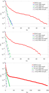 |
Fig. 1 Convergence history of GMRES for the iterative solution of linear system (4), modeling the Ca I 4227 Å (upper panel), Sr II 4077 Å (middle panel), and Mg II h&k lines (lower panel), including PRD effects in the general AD case. We exploit different preconditioners and a zero-vector initial guess, reporting in square brackets the number of outer iterations to convergence (its). The horizontal dashed line represents the tolerance of 10−8. |
Number of outer GMRES iterations (its) and average number of inner GMRES iterations (itsP), exploiting different preconditioners (P) and a zero-vector initial guess (IG).
Number of outer GMRES iterations to convergence (its), exploiting different initial guesses (IG) with no preconditioning (P).
5.3 Combined impact of preconditioning and the initial guess
We next analyzed the combined impact of preconditioners and initial guesses by considering the GMRES solution of Eq. (4) with different settings. For the sake of simplicity, we only analyzed the case where both the initial guess and the preconditioner are constructed with the same low-cost model.
Table 5 reports the number of outer and inner iterations to convergence for different combinations of preconditioners and initial guesses, considering the modeling of the Ca I 4227 Å, Sr II 4077 Å, and Mg II h&k lines, respectively. In all cases, we note that the application of the preconditioner is predominant with respect to the use of a nonzero initial guess. With a suitable initial guess, the preconditioned GMRES method usually requires one iteration fewer than with the zero-vector initial guess.
Number of outer GMRES iterations (its) and average number of inner GMRES iterations (itsP), exploiting different preconditioners (P) and different initial guesses (IG).
6 Conclusions
In this work we have exploited an innovative approach to designing efficient physics-based preconditioners and initial guesses tailored to the iterative solution of computationally challenging linear transfer problems of polarized radiation. As benchmark problems, we considered the modeling of three different chromospheric lines in a 1D semi-empirical atmospheric model, accounting for PRD effects in scattering processes, with a general AD treatment.
By devising physics-based preconditioners and initial guesses, we considerably improved the convergence of the iterative method, ensuring a fast solution of the considered linear transfer problems. Numerical experiments show that a suitable initial guess is able to enhance the un-preconditioned GMRES solution efficiency, but usually by a factor of less than 2. More impressive is the impact of well-constructed preconditioners, which can reduce the number of iterations to convergence by a factor of 10–20. When the two strategies are combined, the effect of a suitable preconditioning clearly prevails over the impact of the initial guess. Given these results, a zero initial guess is still a viable option if an effective preconditioner is provided. To be effective, the preconditioner should provide a good approximation for the intensity. This is because, under typical solar conditions, the feedback of Q, U, and V on the intensity is usually negligible. It is essential that the preconditioner include an appropriate description of the scattering processes (e.g., it accounts for PRD effects, even under the AA approximation, if they have an important impact on the intensity profile), while it can safely neglect polarization. In all the considered cases, using a preconditioner does not affect the accuracy of the converged solution or the behavior of emerging profiles.
We note that the design of efficient iterative schemes can be crucial in the case of more complex settings, such as for 3D geometries, which can be incredibly challenging from the computational point of view (see, e.g., Štěpán & Trujillo Bueno 2013; Benedusi et al. 2023). We stress that the effectiveness of physics-based preconditioners strongly depends on their ability to cheaply capture the dominant physical processes of the problem under consideration. Therefore, this strategy allows us to fully exploit the expertise of the radiative transfer community in the search for the most effective preconditioners.
Although we only focused on a specific model problem, this innovative approach to numerical radiative transfer is general. This work is meant to pave the way for the development of a variety of effective preconditioners for a larger class of problems. Finally, although we only considered the GMRES method, the approach to preconditioning described in this article can certainly be applied to other iterative algorithms, including the traditional fixed-point iterative method (also known as the Richardson iteration method).
Acknowledgements
The financial support by the Swiss National Science Foundation (SNSF) through grant CRSII5_180238 is gratefully acknowledged. Special thanks are extended to L. Belluzzi for particularly enriching discussions.
References
- Alsina Ballester, E., Belluzzi, L., & Trujillo Bueno, J. 2017, ApJ, 836, 6 [Google Scholar]
- Alsina Ballester, E., Belluzzi, L., & Trujillo Bueno, J. 2022, A&A, 664, A76 [NASA ADS] [CrossRef] [EDP Sciences] [Google Scholar]
- Anusha, L., Nagendra, K., Paletou, F., & Léger, L. 2009, ApJ, 704, 661 [NASA ADS] [CrossRef] [Google Scholar]
- Badri, M., Jolivet, P., Rousseau, B., & Favennec, Y. 2018, J. Comput. Phys., 360, 74 [NASA ADS] [CrossRef] [Google Scholar]
- Badri, M., Jolivet, P., Rousseau, B., & Favennec, Y. 2019, Comput. Math. Appl., 77, 1453 [Google Scholar]
- Belluzzi, L., & Trujillo Bueno, J. 2014, A&A, 564, A16 [NASA ADS] [CrossRef] [EDP Sciences] [Google Scholar]
- Benedusi, P., Janett, G., Belluzzi, L., & Krause, R. 2021, A&A, 655, A88 [NASA ADS] [CrossRef] [EDP Sciences] [Google Scholar]
- Benedusi, P., Janett, G., Riva, G., Belluzzi, L., & Krause, R. 2022, A&A, 664, A197 [NASA ADS] [CrossRef] [EDP Sciences] [Google Scholar]
- Benedusi, P., Riva, S., Zulian, P., et al. 2023, J. Comput. Phys., 479, 112013 [NASA ADS] [CrossRef] [Google Scholar]
- Bommier, V. 1997a, A&A, 328, 706 [NASA ADS] [Google Scholar]
- Bommier, V. 1997b, A&A, 328, 726 [NASA ADS] [Google Scholar]
- Bommier, V. 2017, A&A, 607, A50 [NASA ADS] [CrossRef] [EDP Sciences] [Google Scholar]
- Casini, R., & Landi Degl’Innocenti, E. 2008, Astrophys. Plasmas, 44, 247 [NASA ADS] [Google Scholar]
- Casini, R., Landi Degl'Innocenti, M., Manso Sainz, R., Land i Degl’Innocenti, E., & Landolfi, M. 2014, ApJ, 791, 94 [NASA ADS] [CrossRef] [Google Scholar]
- Casini, R., del Pino Alemán, T., & Manso Sainz, R. 2017a, ApJ, 835, 114 [NASA ADS] [CrossRef] [Google Scholar]
- Casini, R., del Pino Alemán, T., & Manso Sainz, R. 2017b, ApJ, 848, 99 [NASA ADS] [CrossRef] [Google Scholar]
- Fontenla, J. M., Avrett, E. H., & Loeser, R. 1993, ApJ, 406, 319 [Google Scholar]
- Ipsen, I. C., & Meyer, C. D. 1998, Am. Math. Monthly, 105, 889 [CrossRef] [Google Scholar]
- Janett, G., & Paganini, A. 2018, ApJ, 857, 91 [Google Scholar]
- Janett, G., Carlin, E. S., Steiner, O., & Belluzzi, L. 2017, ApJ, 840, 107 [NASA ADS] [CrossRef] [Google Scholar]
- Janett, G., Steiner, O., & Belluzzi, L. 2018, ApJ, 865, 16 [NASA ADS] [CrossRef] [Google Scholar]
- Janett, G., Ballester, E. A., Guerreiro, N., et al. 2021a, A&A, 655, A13 [NASA ADS] [CrossRef] [EDP Sciences] [Google Scholar]
- Janett, G., Benedusi, P., Belluzzi, L., & Krause, R. 2021b, A&A, 655, A87 [NASA ADS] [CrossRef] [EDP Sciences] [Google Scholar]
- Landi Degl’Innocenti, E., & Landolfi, M. 2004, Astrophys. Space Sci. Lib., 307, 1 [Google Scholar]
- Leenaarts, J., Pereira, T., & Uitenbroek, H. 2012, A&A, 543, A109 [NASA ADS] [CrossRef] [EDP Sciences] [Google Scholar]
- Liesen, J., & Tichý, P. 2004, GAMM-Mitteilungen, 27, 153 [CrossRef] [Google Scholar]
- Meurant, G., & Duintjer Tebbens, J. 2020, Krylov Methods for Nonsymmetric Linear Systems: From Theory to Computations (Berlin: Springer) [CrossRef] [Google Scholar]
- Mihalas, D. 1978, Stellar Atmospheres, 2nd edn. (San Francisco: W.H. Freeman and Company) [Google Scholar]
- Pearson, J. W., & Pestana, J. 2020, GAMM-Mitteilungen, 43, e202000015 [CrossRef] [Google Scholar]
- Pereira, T. M. D., & Uitenbroek, H. 2015, A&A, 574, A3 [NASA ADS] [CrossRef] [EDP Sciences] [Google Scholar]
- Ren, K., Zhang, R., & Zhong, Y. 2019, J. Comput. Phys., 399, 108958 [NASA ADS] [CrossRef] [Google Scholar]
- Saad, Y. 2003, Iterative Methods for Sparse Linear Systems (USA: SIAM) [Google Scholar]
- Sampoorna, M., Nagendra, K. N., & Stenflo, J. O. 2017, ApJ, 844, 97 [NASA ADS] [CrossRef] [Google Scholar]
- Stenflo, J. 1994, Solar Magnetic Fields: Polarized Radiation Diagnostics, 189 (Berlin: Springer) [Google Scholar]
- Štěpán, J. 2008, Theses, Observatoire de Paris, France [Google Scholar]
- Štěpán, J., & Trujillo Bueno, J. 2013, A&A, 557, A143 [NASA ADS] [CrossRef] [EDP Sciences] [Google Scholar]
- Sukhorukov, A. V., & Leenaarts, J. 2017, A&A, 597, A46 [NASA ADS] [CrossRef] [EDP Sciences] [Google Scholar]
- Trujillo Bueno, J., & Manso Sainz, R. 1999, ApJ, 516, 436 [NASA ADS] [CrossRef] [Google Scholar]
- Trujillo Bueno, J., Landi Degl'Innocenti, E., & Belluzzi, L. 2017, Space Sci. Rev., 210, 183 [CrossRef] [Google Scholar]
- Trujillo Bueno, J., & del Pino Alemán, T. 2022, ARA&A, 60, 415 [NASA ADS] [CrossRef] [Google Scholar]
- Warsa, J., Thompson, K., & Morel, J. 2003, Trans. Am. Nucl. Soc., 449, 25 [Google Scholar]
- Wathen, A. J. 2015, Acta Numer., 24, 329 [CrossRef] [Google Scholar]
In radiative transfer problems, the spatial discretization is usually provided by the considered atmospheric model.
In the multigrid context, Ã corresponds to coarser discretizations.
In general, the SEEs for such a multilevel atomic model (NL > 2) do not have an analytic solution. Therefore, the problem cannot be formulated through the redistribution matrix formalism, and it cannot be linearized in the form of linear system (4).
All Tables
Complexity of the application of different operators appearing in linear system (4).
Labels of the different simplified settings used to design both preconditioners and initial guesses for the iterative solution of the full problem, which considers polarization phenomena and accounts for PRD effects in the general AD case.
Number of outer GMRES iterations (its) and average number of inner GMRES iterations (itsP), exploiting different preconditioners (P) and a zero-vector initial guess (IG).
Number of outer GMRES iterations to convergence (its), exploiting different initial guesses (IG) with no preconditioning (P).
Number of outer GMRES iterations (its) and average number of inner GMRES iterations (itsP), exploiting different preconditioners (P) and different initial guesses (IG).
All Figures
|
Fig. 1 Convergence history of GMRES for the iterative solution of linear system (4), modeling the Ca I 4227 Å (upper panel), Sr II 4077 Å (middle panel), and Mg II h&k lines (lower panel), including PRD effects in the general AD case. We exploit different preconditioners and a zero-vector initial guess, reporting in square brackets the number of outer iterations to convergence (its). The horizontal dashed line represents the tolerance of 10−8. |
| In the text | |
Current usage metrics show cumulative count of Article Views (full-text article views including HTML views, PDF and ePub downloads, according to the available data) and Abstracts Views on Vision4Press platform.
Data correspond to usage on the plateform after 2015. The current usage metrics is available 48-96 hours after online publication and is updated daily on week days.
Initial download of the metrics may take a while.