| Issue |
A&A
Volume 682, February 2024
|
|
|---|---|---|
| Article Number | A103 | |
| Number of page(s) | 10 | |
| Section | Astrophysical processes | |
| DOI | https://doi.org/10.1051/0004-6361/202347836 | |
| Published online | 07 February 2024 | |
Detection of the relativistic Shapiro delay in a highly inclined millisecond pulsar binary PSR J1012−4235
1
Max-Planck-Institut für Radioastronomie, Auf dem Hügel 69, 53121 Bonn, Germany
2
National Radio Astronomy Observatory, 520 Edgemont Rd., Charlottesville, VA 22903, USA
e-mail: This email address is being protected from spambots. You need JavaScript enabled to view it.
3
Centre for Astrophysics and Supercomputing, Swinburne University of Technology, PO Box 218 VIC 3122, Australia
4
ARC – Centre of Excellence for Gravitational Wave Discovery (OzGrav), Swinburne University of Technology, PO Box 218 VIC 3122, Australia
Received:
30
August
2023
Accepted:
28
October
2023
Abstract
PSR J1012−4235 is a 3.1 ms pulsar in a wide binary (37.9 days) with a white dwarf companion. We detect, for the first time, a strong relativistic Shapiro delay signature in PSR J1012−4235. Our detection is the result of a timing analysis of data spanning 13 yr and collected with the Green Bank, Parkes, and MeerKAT Radio Telescopes and the Fermiγ-ray space telescope. We measured the orthometric parameters for Shapiro delay and obtained a 22σ detection of the h3 parameter of 1.222(54) μs and a 200σ detection of ς of 0.9646(49). With the assumption of general relativity, these measurements constrain the pulsar mass (Mp = 1.44−0.12+0.13 M⊙), the mass of the white dwarf companion (Mc = 0.270−0.015+0.016 M⊙), and the orbital inclination (i = 88.06−0.25+0.28 deg). Including the early γ-ray data in our timing analysis facilitated a precise measurement of the proper motion of the system of 6.58(5) mas yr−1. We also show that the system has unusually small kinematic corrections to the measurement of the orbital period derivative, and therefore has the potential to yield stringent constraints on the variation of the gravitational constant in the future.
Key words: relativistic processes / binaries: general / stars: neutron / pulsars: individual: PSR J1012–4235 / gamma rays: stars
© The Authors 2024
 Open Access article, published by EDP Sciences, under the terms of the Creative Commons Attribution License (https://creativecommons.org/licenses/by/4.0), which permits unrestricted use, distribution, and reproduction in any medium, provided the original work is properly cited.
This article is published in open access under the Subscribe to Open model .
Open Access funding provided by Max Planck Society.
1. Introduction
Due to their rotational stability and high spin frequencies, millisecond pulsars (MSPs) provide remarkable timing precision and have therefore proven to be excellent probes of gravity theories and the physics of dense matter in neutron stars (NSs; see Özel & Freire 2016), and have been used to constrain the nHz gravitational wave background (Agazie et al. 2023; Reardon et al. 2023; EPTA Collaboration 2023; Xu et al. 2023). These diverse applications are a result of modelling the physical phenomena that influence the times of arrival (ToAs) of pulses at the telescope or receiver.
In the case of binary pulsars, the modelling of the ToAs can lead to the detection of several relativistic effects, which either appear as deviations from the Keplerian orbital motion of the pulsar, or as additions to the propagation time of the radio waves to the Earth. These relativistic effects can be quantified (and therefore parameterised) in a theory-independent way with the so-called “post-Keplerian (PK) parameters” (Damour & Taylor 1992). Assuming a theory of gravity, such as general relativity (GR), these PK parameters become functions of the Keplerian parameters of the orbit of the pulsar as well as its mass and that of its companion. Therefore, measurements of two PK parameters can – with the assumption of a specific gravity theory – directly constrain the masses of the two component stars of the system. A detection of three or more PK parameters will provide additional ways to determine the same two masses, providing consistency tests of the gravity theory being assumed (see e.g. Kramer et al. 2021a, and references therein).
In this work, we discuss our timing analysis of the MSP system PSR J1012−4235, and our detection of a Shapiro delay (Shapiro 1964) in its timing. This effect is observed when the radio pulses are delayed as they propagate through a space-time curved by the pulsar’s companion; it is more easily observed in edge-on binaries, where the companion passes close to the pulsar’s line of sight. The variation of the Shapiro delay with orbital phase allows the measurement of two PK parameters (see details below), which are sufficient for a determination of the component masses (Shamohammadi et al. 2023).
PSR J1012−4235 is a 3.1 ms pulsar discovered using the Parkes radio telescope in a survey (Camilo et al. 2015) that targeted unidentified γ-ray sources found with the Large Area Telescope (LAT; Atwood et al. 2009) on board the Fermiγ-ray space telescope. In the discovery paper, by fitting for the changes in the barycentric period due to changes in the Doppler shift (caused by the changing orbital velocity), the orbital parameters of the binary were determined, although with low precision. The pulsar has a low-eccentricity (e < 0.001) orbit with a period of 37.9 days around a companion with a minimum mass of 0.26 M⊙. This suggests it is likely a helium-core white dwarf (He WD). This minimum companion mass is very close to the companion mass predicted by Tauris & Savonije (1999) for a He WD companion for a system with this orbital period. This indicates that, if the companion is indeed a He WD and the model is correct, the system is probably being viewed edge-on, that is, with an orbital inclination (i) of close to 90 deg.
From 2013 to 2015, additional timing observations were carried out with the 64 m Parkes “Murriyang” radio telescope and the Green Bank Telescope (GBT), and a phase-connected timing solution was derived with much improved constraints on the position, spin-down, and orbital parameters. The eccentricity and orbital period of the system were found to be consistent with the MSP-He WD relationship given by Phinney & Kulkarni (1994).
The detection of the Shapiro delay in this system, made possible by the high sensitivity of the MeerKAT telescope (Jonas & MeerKAT Team 2016), confirmed the high predicted orbital inclination. This 64-dish array provides excellent timing sensitivity for pulsars in the southern hemisphere (Bailes et al. 2020). With the aim of performing high-precision timing for a large number of pulsar systems, a Large Science Project (LSP) called MeerTIME (Bailes et al. 2016, 2020) is being carried out. One program under this project is the relativistic binary program (referred to as “RelBin”). RelBin specifically targets relativistic binary pulsars for the purpose of measuring relativistic effects, constraining NS masses, and testing GR, along with constraining alternative theories of gravity (Kramer et al. 2021b). Another MeerTIME program is the “pulsar timing array” (PTA), the aim of which is to use MSPs for the detection of nHz gravitational waves (Parthasarathy et al. 2021; Spiewak et al. 2022; Miles et al. 2023). The PSR J1012−4235 system was observed regularly from 2019 to 2022 under the PTA and RelBin programs.
In this paper, we present a phase-connected timing solution for PSR J1012−4235, which in this case is derived from the timing observations obtained with the Parkes, GBT, and MeerKAT radio telescopes, and γ-ray data collected by Fermi-LAT. We obtained precise measurements of the proper motion, position, and orbital parameters. The detection of a strong Shapiro delay signature was made possible by dedicated orbital campaigns carried out under the RelBin program, especially around superior conjunction and the extrema of the unabsorbed component of the Shapiro delay signal. This provides good measurements of the orbital inclination of the binary and the pulsar and companion masses.
The present paper is organised as follows: in Sect. 2 we describe the radio data set used for the analysis in this work, in Sect. 3 we discuss the data reduction procedure of both radio and γ-ray data, and in Sect. 4 we discuss the polarisation profile of the pulsar and the fit of its linear polarisation using the Rotating Vector Model (RVM; Radhakrishnan & Cooke 1969). In Sect. 5 we discuss the timing analysis and its results, in Sect. 6 we discuss the γ-ray pulse profile and compare its features with the radio profile, and finally in Sect. 7 we summarise our results.
2. Observations
We now describe the radio data set analysed in this work. The details of all the radio observations used in this work are listed in Table 1.
Details of radio observations.
2.1. Parkes and GBT observations
Discovery observations and follow-up timing observations (continued until January 2015) of this pulsar were carried out with the Parkes radio telescope. Stokes-I data were recorded in search mode with the central beam of the 20 cm multi-beam receiver (Staveley-Smith et al. 1996). For a detailed description of this data set, we refer the reader to Kerr et al. (2012) and Camilo et al. (2015).
To further refine the timing solution of the pulsar, timing observations were also carried out with the GBT in 2013 and 2014. For these observations, search-mode data were obtained with the 820 MHz receiver covering 200 MHz of bandwidth. Only Stokes-I data were recorded, which were sampled at 40.96 μs with 2048 frequency channels.
2.2. MeerKAT observations
The instrumentation and setup for pulsar observations with MeerKAT are explained in detail in Bailes et al. (2020). The timing observations with MeerKAT for this pulsar were performed as part of both PTA and RelBin programs. All the observations were carried out with the L-band receiver and used the PTUSE backend (Bailes et al. 2020). Typical observation times of PTA observations were ∼5 min, while RelBin observations (which focused on getting a better orbital coverage) were typically ∼34 min. In addition, we carried out one long observation of ∼5 h covering superior conjunction under the RelBin program. All the observations covered an effective bandwidth of 775.75 MHz divided across 928 frequency channels. The MeerKAT data used in this work were taken from April 2019-January 2022, and amounted to a total of 73 observations covering 13.2 h. The integrated pulse profile from MeerKAT observations is shown in Fig. 1.
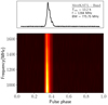 |
Fig. 1. MeerKAT L-Band profile obtained by integrating a total of 13.2 h of data. Top plot: Intensity versus rotation phase. Bottom plot: Radio frequency versus rotation phase. In this latter plot, we can see how the pulse profile evolves with radio frequency. The number of phase bins was 1024 and the S/N is 977. |
3. Data reduction
3.1. Radio data
All the earlier Parkes and GBT data available in the folded psrchive format were reloaded with a consistent phase-connected timing solution in order to improve the signal-to-noise ratio (S/N) of the pulse profiles. To enhance the S/N of individual ToAs, each Parkes epoch was integrated in frequency, while two frequency sub-bands were formed for each GBT epoch.
The entire MeerKAT data reduction was performed using the standard pulsar analysis software PSRCHIVE1 (Hotan et al. 2004; van Straten et al. 2012). All the MeerKAT L-Band data were passed through a data-reduction pipeline: MEERPIPE2 (Parthasarathy et al. 2021), which first performs the RFI excision using a modified version of COASTGUARD (Lazarus et al. 2016), and then carries out the polarisation and flux calibration. In this process, to remove the low power levels at the edges of the bandpass, all the observations were reduced from their original bandwidth of 856–775.75 MHz. The pipeline outputs a consistent data set, with similar bandwidth and central frequency, which can be readily used for the timing analysis.
To calculate the pulse ToAs of all high-S/N integrations in the MeerKAT data, we cross-correlated them with a standard template of the pulse profile. As the intrinsic profile shape of a pulse can vary with frequency – and this is certainly the case for PSR J1012−4235, as we see in Fig. 1, using a single template created by integrating in frequency can smear some of the profile features and lead to increased ToA uncertainty. Therefore, a template with multiple frequency sub-bands can provide smaller ToA uncertainties. Additionally, sharp features in the profiles with different polarisation can help improve the timing precision further, and therefore a template with non-integrated polarisation can be useful in some cases. In order to identify the best-suited standard template for our case, and one that would give the smallest residual RMS from the fit, we created four different types of template and produced ToAs with each of them:
-
1F1P: Simple one-dimensional profile, where we integrated in both frequency and polarisation, created with the paas routine of psrchive.
-
8F1P: Eight-frequency band profile, sub-banded to eight frequency channels and integrated completely in polarisation; to generate ToAs in this case we used the Fourier domain with Markov chain Monte Carlo (FDM) algorithm of the pat routine.
-
1F4P: One-dimensional profile with polarization information. We integrated in frequency but with full Stokes parameter profiles created using the matrix template matching (MTM) algorithm of the pat routine to generate ToAs.
-
8F4P: Sub-banded to eight frequency channels and non-integrated polarisation profiles with full Stokes parameters.
In addition to these, templates with four rather than eight frequency channels in schemes (ii) and (iv) were also created for comparison. We find that the best template for MeerKAT data that provides minimum parameter uncertainties for our dataset is (2), that is, integrated in polarisation but sub-banded to eight frequency channels. For the earlier dataset (both Parkes and GBT), the best resulting reduced  comes from individual templates formed with integrated frequency.
Datasets taken from different telescopes (GBT, Parkes, and MeerKAT in this case) lead to additional time delays due to different instruments, which differ both in terms of their design and their geographic location. To account for these delays, we fit for an arbitrary phase offset (“JUMPS”) between each telescope datum. Additionally, an inconsistent definition of templates can lead to unreliable prediction of orbital parameters and high timing parameter uncertainties (as discussed in detail in Guo et al. 2021). For this reason, we aligned all three standard templates created for the three datasets with a consistent phase reference point.
Typically, for MeerKAT data, we generated ToAs for one-minute subintegrations, leading to eight ToAs per minute. The total number of ToAs extracted from each data set is given in Table 1. The table also provides values for the EFAC parameter, which is used to rescale the uncertainties of ToAs in order to avoid unmodelled systematic effects; it was calculated so that the reduced χ2 of the fit for each data set is 1. This increase in the ToA uncertainties results in more conservative estimates of the uncertainties of the timing parameters.
3.2. γ-ray data
The Parkes survey by Camilo et al. (2015) was designed to search for unidentified γ-ray sources. PSR J1012−4235 was found in the γ-ray source 3FGL J1012−4235 presented in the third Fermi-LAT catalogue (Acero et al. 2015). With the preliminary timing solution obtained using only radio data, we can see that, as is the case for ∼300 other pulsars (Smith et al. 2023), PSR J1012−4235 is pulsating in γ-rays, confirming the association between the radio pulsar and the γ-ray source.
To determine the likelihood of each photon being a signal or background, we applied a simplified weighted method developed by Bruel (2019), which considers factors such as photon energy and angular separation from the pulsar position. This method allowed us to assign a probability (or weight) to each photon for the length of the entire Fermi mission – more specifically, from Mission Elapsed Time (MET) 239558000 (MJD 54682.66202546) and MET 667972000 (MJD 59641.15734954) – within the 0.1–3 GeV energy range and within 1° of the pulsar position.
Using the weighted photon set, we calculated the pulse phase for every γ-ray photon based on the best radio timing solution available, using the TEMPO2 Fermi plugin3. We examined the resulting folded γ-ray profile to assess the adequacy of the initial timing solution for further analysis.
As discussed in Sect. 6, this folded γ-ray profile is characterised by a double peak consisting of strong and narrow pulses. These provide precise, albeit sparse γ-ray ToAs: in total, we extracted 32 γ-ray ToAs (each with uniform S/N) using a multi-component Gaussian template employing the maximum likelihood methods described in Ray et al. (2011). These ToAs nicely complement the radio data, and are especially useful for constraining parameters with long-term trends in residuals, such as the spin-period derivative and the proper motion. Their addition especially helps to constrain long-term DM variations to which the γ-ray ToAs are immune. They also confirm that we have not missed a single rotation in the four-year gap of radio observations between 2015 and 2019.
4. Polarisation
As for almost all MSPs with nearly circular orbits, the spin axis of the pulsar is likely to be aligned with the orbital angular momentum; the reason for this is that the pulsar was spun up from orbiting material, and there has been no violent event to change the orbital plane (Tauris & van den Heuvel 2023). The high inclination angle of the system (see discussion in Sect. 5) therefore implies that our line of sight to the system is nearly perpendicular to the spin axis, which suggests the possibility that the pulsar is an orthogonal rotator. In such cases, we should expect to see emission from both magnetic poles in the form of an inter-pulse about 180 deg away from the main pulse.
Figure 2 shows the polarisation-calibrated profile of this pulsar created by integrating all the 73 observations covering a total of 13.2 h of MeerKAT L-band data. A description of the polarisation calibration of the MeerKAT data of this pulsar is provided by Spiewak et al. (2022); the linear polarisation was derotated using the pulsar’s well-known rotation measure (RM) of 61.80 rad m−2.
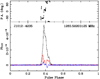 |
Fig. 2. Polarisation calibrated profile of PSR J1012−4235 formed from MeerKAT L-band data. Bottom panel: Intensity in arbitrary units as a function of rotational phase. The red colour shows linear polarisation and the blue colour shows circular polarisation across the rotational phase. Top panel: Variation of the position angle of the linear polarisation with spin phase. |
Only 11% of the total flux is polarised, of which the majority is linearly polarised, with a fractional linear polarisation of L/I = 23%, and a fractional circular polarisation of V/I = 1.7% (|V|/I = 6.3%). The circular polarisation reverses its sign exactly at the centre of the on-pulse region. The position angle (PA) swing (see top panel of Fig. 2) shows steep transitions, which are likely caused by changes between orthogonal polarisation modes (OPMs). As we can see in Fig. 2, all flux is concentrated in a narrow region, with no additional low-level components detectable anywhere else. After reducing the detection threshold for total intensity and polarised components, we can confirm that we do not detect any signature of the expected inter-pulse, which would be seen as emission at both poles. This refutes the idea of a simple orthogonal rotator.
In order to gain some independent insight into the geometry of the system, we performed an RVM (see Radhakrishnan & Cooke 1969) fit to the variation of the PA of linear polarisation with spin phase. Given the unknown complexities of the emission of radio pulsars, these results should be taken with some caution.
We performed the fit as described in Guo et al. (2021), to which we refer for further details. Briefly, we determined the geometry of the pulsar by fitting the RVM model using a Bayesian optimisation method as described by Johnston & Kramer (2019) and Kramer et al. (2021b). For this fit, we need four parameters, where the most important are the angle between the spin axis and the magnetic axis (α), and the angle between the line of sight and the spin axis (ζ), which is given by ζ = α + β, where β is the minimum angle between the line of sight and the magnetic axis. The other two angles are Φ0, the spin phase where the magnetic pole is closest to the line of sight, and Ψ0, which is the position angle of the linear polarisation at Φ0. In our modelling, we constrain ζ by determination of the orbital inclination (from the assumption that the spin and orbital angular momenta are aligned). For the other parameters, we use uniform priors. The code we used allows the possible existence of OPMs, that is, sudden 90 deg jumps in the PA values. The resulting parameters and their correlations are shown in Fig. 3.
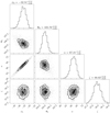 |
Fig. 3. Corner plot with the parameters of the RVM fit to the polarisation profile of PSR J1012−4235. Φ0 is the spin phase where the magnetic pole is closest to the line of sight, Ψ0 is the position angle of the linear polarisation at Φ0, α is the angle between the spin axis and the magnetic axis, and ζ is the angle between the line of sight and the spin axis, which is given by ζ = α + β, where β is the minimum angle between the line of sight and the magnetic axis. |
In the middle panel of Fig. 4, we can see how the prediction of this model compares with the observed PA of the linearly polarised emission as a function of spin phase, with the lower panel displaying the differences (residuals). As we can see, the observed PA follows the model reasonably well: the sudden 90 deg changes in the PA are, as mentioned above, likely to be caused by changes of dominant OPMs. This notion is supported by the simultaneous drops in linear polarisation at those longitudes. Apart from these drops, the PA changes slowly with spin phase.
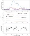 |
Fig. 4. RVM fit with the polarised pulse profile. Top plot: Zoom into the region of the radio pulse of PSR J1012−4235; we can see more clearly how the polarised emission changes with spin phase, or longitude. The colours are as in Fig. 2. Middle plot: Position angle as a function of the longitude. The black dots indicate the measured PA angles for the linearly polarised emission, and the smooth red curves (solid and dashed) indicate the prediction of the best-fit model. Polarisations that are 180 deg apart are identical. Polarisations 90 deg apart correspond to changes to OPMs. Lower plot: Differences between the measured PAs and the nearest model prediction accounting for possible OPM changes, i.e. the PA residuals. |
In the best-fit model, the reason for this slow change is that, even at closest approach, the magnetic axis passes far (β ∼ 20 deg) away from the line of sight. The fitted α ∼ 67 deg shows that this pulsar is not an orthogonal rotator (which would require α ∼ 90 deg). This also means that we are looking at the edge of a wide (> 20 deg) emission cone. To some extent, this could explain why we see no inter-pulse: if the emission cone at the other magnetic pole is not as wide, we will not see radio emission from it.
However, even if the emission cone from the other magnetic pole is as wide as the cone from the pole we see, we might still miss it. This is because, in this system, the best-fit value of Φ0 at a longitude of ∼106 deg is, unusually, before the start of the phase of strong radio emission. This geometry means that the earlier half of this emission cone has no associated emission; that is, it is clear that this emission cone is not fully illuminated. If this is the case, then the same might be happening in the parts of the emission cone from the other pole that cross our line of sight.
In summary, although the orbital inclination is close to 90 deg, the pulsar is not an orthogonal rotator, a condition that is common among the systems timed by RelBin (Kramer et al. 2021b). The fact that we see radio emission at > 20 deg from the magnetic field axis is common among MSPs, which generally have wide emission patterns (as shown by their generally long and complex pulse profiles). These broad emission patterns result in their large (∼1) beaming fractions.
The Shapiro delay measures only sin i. This means that for each measurement of sin i, there are two possible solutions for i that are equidistant from edge-on (90 deg). We repeated the polarisation analysis for ζ ∼ 92 deg, and obtain very similar results: in this case, we obtain α ∼ 71 deg, which again results in β ∼ 20 deg. The quality of the fit is indistinguishable from the previous case (ζ ∼ 88 deg), which means that the polarimetry data do not allow a choice between the two possible values of the orbital inclination.
5. Timing analysis
For the timing analysis, we used pulsar timing software TEMPO4, because the specific orbital model we use in the analysis (i.e. ELL1H+, discussed in Sect. 5.1) is only available in this timing package. The software first transfers all the ToAs from UTC to terrestrial time standard “TT(BIPM)”, which is defined by the International Astronomical Union (IAU). We use NASA’s JPL Solar System ephemeris, DE436 (Folkner & Park 2016), to account for the motion of the Earth. For each ToA, the varying position of the radio telescope relative to the Solar System Barycentre (SSB) was then used to calculate the barycentric times of arrival. TEMPOthen calculates the phase residuals of each of the ToAs by comparing them to ToAs predicted by an initial timing model; we used the ephemeris presented in Camilo et al. (2015) as our initial model. TEMPOthen adjusts the timing parameters to minimise the residual χ2. To compensate for the underestimated ToA uncertainties, which are possibly due to left-over systematic effects, we used separate weighting factors for each dataset; these are multiplied by their respective ToA uncertainties before the fit (see Table 1).
5.1. Binary models
To fit for the binary parameters, we used the ELL1H+ binary model (Guo et al. 2021), which is implemented in the latest versions of TEMPO (> 13.102). This is a theory-independent model based on the ELL1 model (Lange et al. 2001), which is designed to avoid the correlation between the epoch of periastron, T0, and the longitude of periastron, ω, in low-eccentricity binaries by reparameterising the orbit and measuring the epoch of the ascending node, Tasc, instead of T0. Instead of fitting for ω and the orbital eccentricity e, this model fits for the Laplace-Lagrange parameters: ϵ1 = e cos ω and ϵ2 = e sin ω. In addition to the ELL1 model, the ELL1H+ model includes an extra term of the order of xe2 in the expansion of the Römer delay (Zhu et al. 2019), which makes it applicable to most binary pulsars. As the next-order term for PSR J1012−4235 – namely 𝒪(xe3) ∼ 0.9 ns – is much smaller than the uncertainty in our measurement of the h3 parameter (∼55 ns), ignoring it does not affect our measurement of the Shapiro delay.
The ELL1 model measures the Shapiro delay in the form of two PK parameters, namely range (r) and shape (s), which according to GR are given by r = T⊙Mc and s = sin i and where  s is an exact quantity, and represents the solar mass parameter (
 ; Prša et al. 2016) in time units. The ELL1H+ model instead uses the orthometric parameterisation of Shapiro delay (Freire & Wex 2010), which removes the high correlation between the r and s parameters, leading to a robust quantification of this effect. The Shapiro delay parameters are the orthometric amplitude, h3, and the orthometric ratio, ς, which in GR are given by:
 (1)
(1)
To fit for these parameters, the ELL1H+ model uses the exact expression for the Shapiro delay, that is, Eq. (29) in Freire & Wex (2010).
5.2. Results from radio and γ-ray timing
From the fit of the ELL1H+ binary model to all the radio and γ-ray data, we derived a phase-connected timing solution for this system (see Table 2). This is a unique solution for the binary that correctly predicts the pulse arrival times for every rotation of the pulsar in the data set. Figure 5a shows the post-fit ToA residuals as a function of time. The addition of Fermi-LAT ToAs (detailed in Sect. 3.2) is especially useful in precisely constraining the long-term astrometric parameters for the system. We get a reduced χ2 of 1.0084 after adding the EFAC parameter. The resulting residuals show a Gaussian distribution with no trends (or structure), indicating that there are no detectable unmodelled effects.
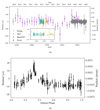 |
Fig. 5. Residuals obtained from the fit of the timing model for PSR J1012−4235. Top plot: Post-fit residuals showing ToAs from Parkes, GBT, MeerKAT, and Fermi-LAT data, with error bars representing 1σ uncertainty in ToAs. Bottom plot: Residuals of MeerKAT ToAs, excluding the fit for Shapiro delay effect but fixing all the other system and orbital parameters obtained from the full fit. The orbital phase is measured from periastron and the peak in the Shapiro delay signature occurs around the phase of superior conjunction of the pulsar. |
Phase-connected timing solution for PSR J1012−4235, making use of combined radio and γ-ray data.
The resulting best-fit solution includes precise astrometric, spin, and orbital parameters. The astrometric parameters include a precise proper motion in right ascension (RA) and declination (Dec) directions, resulting in a total heliocentric proper motion (μT) of 6.58(5) mas yr−1, as well as a parallax of 0.85(50) mas. This measurement is important, because it excludes one of the distance estimates of the YMW16 model (see Sect. 5.4). The spin parameters include two significant DM derivatives and one spin frequency derivative.
Regarding the orbital parameters, we find a strong detection of Shapiro delay with h3 = 1.222(54) μs and ς = 0.9646(49). The variation of the Shapiro delay with orbital phase can be clearly seen in Fig. 5b. This detection implies a companion mass of Mc = 0.276(16) M⊙, and a sin i = 0.99937(18), meaning an inclination i of  . The pulsar mass (Mp) derived from these measurements using the mass function is 1.44(13) M⊙. Our measurement of the companion mass aligns well with the ∼0.27 M⊙ predicted by the Porb–MWD relationship of Tauris & Savonije (1999) for He WDs. The eccentricity of 3.45 × 10⁻⁴ agrees well with the theoretical range predicted by Phinney & Kulkarni (1994) for a MSP–WD binary with an orbital period of 37.9 days.
Regarding the measurement of the advance of periastron,  in this binary, its prediction from GR gives a value of 6.5 × 10⁻⁴ deg yr−1, while our fit for this parameter yields (1.4 ± 1.5)×10−3 deg yr−1. Although the measurement is consistent with the expected value, its uncertainty is still about two times larger than the expected effect, which means that we cannot yet measure this effect. However, measuring this parameter should be feasible in the near future with continued timing with MeerKAT observations.
5.3. Mass constraint from the Shapiro delay detection
In order to better understand the correlations between the Shapiro delay parameters and better estimate their uncertainties and the uncertainties on the masses and orbital inclination, we performed a Bayesian study of the masses and orbital inclination of the system. First, we created a uniform grid of points on the (cos i − Mc) plane and derived the best-fit χ2 values from the TEMPO fit of this model on each of the points in this grid. Second, these χ2 values are then converted to a Bayesian likelihood using the relation by Splaver et al. (2002):  , where
  is the minimum χ2 value. These likelihoods are then used in the calculation of joint posterior probability density functions (PDFs), both in the original plane and also in the (Mp − Mc) plane.
Figure 6 shows the Shapiro delay parameters derived from the ELL1H+ model on the (cos i − Mc) and (Mp − Mc) planes. Black contours represent the 39% (inner) and 85% (outer) confidence ellipses on the joint posterior PDFs, which represent the 1σ and 2σ error bars in 1D PDFs. Using this method, we get  , implying an inclination of 88.06
 ,
,  M⊙, and
  M⊙, with errors representing 1σ uncertainties. These values and uncertainties agree very well with those derived in Sect. 5.2.
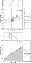 |
Fig. 6. Constraints on Mc, Mp, and cos i derived from the measurement of Shapiro delay. Coloured dashed lines depict the 1σ uncertainty on the measurement. Black contours show the likelihood or 2D PDFs at 39% (inner) and 85% (outer) confidence ellipse from the |

5.4. Kinematic effects on the spin and orbital period
The two most broadly accepted Galactic electron density models are the models YMW16 (Yao et al. 2017) and NE2001 (Cordes & Lazio 2002). These models can predict the distance to the pulsar based on the line-of-sight electron density and the DM of the pulsar. For this pulsar, YMW16 predicts a distance of 0.37 kpc, while NE2001 predicts 2.51 kpc. These estimates are generally thought to be accurate to ∼20%, but in this case it is clear that they do not agree at this level (see Fig. 7). However, in the timing solution, we fit for a parallax and obtain 0.85(50) mas, indicating a distance (d = 1/ϖ) of 1.18 kpc, a value in between the predictions from both the models but more aligned with NE2001 model within 1σ.
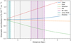 |
Fig. 7. Acceleration contributions to the orbital period derivative due to kinematic effects as a function of distance. Orange and green curves show the vertical and differential accelerations from the Galactic disc, while the red curve shows the contribution from the proper motion of the pulsar. The blue curve represents the total acceleration contribution. A distance uncertainty of 20% is assumed on the DM distance predictions from the NE2001 model (purple shaded region) and the YMW16 model (teal shaded region), while the 1σ uncertainty is shown for the parallax measurement from timing (grey shaded region). |
The observed spin period derivative of the pulsar (Ṗobs) includes contributions not only from the intrinsic spin period derivative but also from the derivative of the Doppler factor. The later includes two terms, representing (a) the proper motion of the pulsar, an effect known as the Shklovskii effect (the first term in the equation below) and (b) the Galactic acceleration (Lorimer & Kramer 2012):
 (2)
(2)
where Ṗint is the intrinsic spin period derivative, agal, disc is the vertical acceleration contribution from the Galactic disc, and agal, rot is the acceleration due to the differential rotation of the galaxy.
These Galactic accelerations are calculated from the analytical expressions given by Damour & Taylor (1991), Nice & Taylor (1995), Lazaridis et al. (2009):
 (3)
(3)
 (4)
(4)
where β ≡ (d/R0) cos b − cos l and zkpc ≡ |d sin b| in kpc. R0 is the distance to the Galactic centre, 8.275(34) kpc, and Θ0 is the Galactic rotation velocity, 240.5(41) km s−1 (values taken from Guo et al. 2021). This approximation is valid given the fact that the pulsar is relatively nearby and likely has a low Galactic height.
Assuming the distance predicted by our parallax measurement, we obtain an acceleration of  for the sum of kinematic corrections. Using this, we get the value of kinematic correction to Ṗ, Ṗkin = 6 × 10⁻²⁴. Thus
  , which is very close to the Ṗobs because Ṗkin is 100–1000 times smaller. With this estimate of Ṗint, we estimate the surface magnetic field, Bs, the characteristic age, τc, and the spin-down luminosity of the system, Ė, of the pulsar using the equations in Lorimer & Kramer (2012). Table 3 presents the estimates for the derived parameters along with their 1σ uncertainties.
Derived astrometric, spin, and orbital parameters for PSR J1012−4235.
Similar kinematic effects to those discussed above affect the measurement of the observed orbital period derivative, Ṗb,obs, as well. Assuming the distance from the parallax, we estimate the total kinematic contribution  . The expected orbital decay due to the quadrupolar GW emission from this system is
  (assuming GR). The observed Ṗb is 1.4 ± 4.3 × 10⁻¹² s s−1. Although this measurement is consistent with expectations, its uncertainty is still two orders of magnitude higher than the expected contributions from kinematic effects and is nearly five orders of magnitude larger than the orbital decay from GW emission. Therefore, we cannot yet constrain the kinematic effects from timing.
Figure 7 shows each of the contributions to Ṗb,obs from the kinematic effects as a function of distance. As we can see, the total contribution to Ṗb from the kinematic effects (blue curve) is extremely flat. This turns out to be one of the most interesting features of this system. Even with the relatively large distance uncertainty, this contribution is not only small but it has a small associated uncertainty, δṖb,kin = 9 × 10⁻¹⁴ s s−1. This has an important consequence: it means we will be able to obtain a tight constraint on the variation of the gravitational constant  (Will 1993; Uzan 2011). Furthermore, this will happen relatively soon, because the precision of Ṗb,obs will continue to improve, and relatively quickly, with the relative error scaling as T−5/2, where T is the timing baseline; it will, in reality, improve even faster because the precise MeerKAT observations started only very recently. This will result in improved estimates of the intrinsic Ṗb, which will only be limited by the Ṗb,kin. The constraint on
  will then be proportional to δṖb,kin/Pb = 8.6 × 10⁻¹³ yr−1.
6. γ-ray and radio pulse profiles
With our new timing solution obtained from radio data, we refolded the γ-ray data to create a γ-ray pulse profile. We use a single phase-connected solution on both the radio and γ-ray data such that the profiles are phase-aligned; that is, the start of the rotational phase indicates the same reference epoch.
Figure 8 shows a comparison of the two profiles. Unlike in radio, we do see a second peak in the pulsed emission, which is superficially consistent with the previously mentioned idea of the orthogonal rotator. However, like the radio polarisation, this γ-ray profile does not support the idea of an orthogonal rotator: the pulse morphology seen here is similar to that of most γ-ray pulsars (Smith et al. 2023), where a single radio pulse, after a small offset in phase (which is visible here), is followed by two strong peaks in the γ-ray emission, linked by a bridge of emission, which is also faintly visible here.
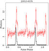 |
Fig. 8. Comparison of the γ-ray pulse profile (red) with the radio profile (black) of PSR J1012−4235. The profile is formed using a phase-connected solution (ephemeris) such that both the folds take the same reference epoch as the start of the profile. |
This is clear evidence supporting the idea that the radio and γ-ray emission do not generally originate from the same region of the pulsar magnetosphere. There are a few exceptions, such as the first MSP (PSR B1937+21) and the first “black widow” pulsar, PSR B1957+20, where both the radio and γ-ray emission show a precisely co-located pulse and inter-pulse (for a detailed discussion on these topics, see e.g., Guillemot et al. 2012). The radio emission of those systems is more consistent with that of an orthogonal rotator. Further analysis in an attempt to constrain the pulsar magnetosphere using γ-ray data will be carried out in the future.
7. Conclusion
In this paper, we present the results of our timing analysis of PSR J1012−4235, which we performed with data obtained with the Parkes (1.5 yr), GBT (7 months), and MeerKAT (2.7 yr) radio telescopes, and the Fermiγ-ray space telescope (13 yr), covering a total time baseline of 13 yr. We present the phase-connected timing solution of this pulsar, including refined estimates of astrometric, kinematic, and orbital parameters. We measured the proper motion of the pulsar to be 6.5 mas yr−1. With the help of dense MeerKAT observations that cover the superior conjunction of the pulsar, we detect a significant Shapiro delay signature in the binary, the first relativistic effect in this system. We obtain a 22σ detection of the h3 parameter of 1.222(54) μs and a ∼200σ detection of ς = 0.9646(49). This yields measurements of the component masses and the orbital inclination:  M⊙,
M⊙,  M⊙, and
  .
.
Using the phase-connected solution, we also phase-aligned the radio- and γ-ray profiles of the pulse. This alignment shows that the pulse peak of the radio profile precedes the peak in the γ profile, which in turn aligns with one of the features of the radio profile.
Lastly, with the proper motion and parallax measurements from timing, we constrained the kinematic contributions to the observed spin period and orbital period derivatives. We note that the curve for the contribution of the kinematic effects to Ṗb,obs is nearly flat within the range of distances allowed by our measurement of the parallax. Therefore, despite the large uncertainty in the distance measurement, we obtain a very small uncertainty in the kinematic contributions to Ṗb. This represents the limiting factor for estimating the intrinsic Ṗb of the system from future timing measurements. Therefore, continued timing of this system might eventually result in a limit on  of 8.6 × 10⁻¹³ yr−1. For PSR J1713+0747, which currently provides the best limit on this parameter, this parameter is 8.1 × 10⁻¹³ yr−1 (Zhu et al. 2019). Thus, the improvement of the Ṗb measurement of PSR J1012−4235 has the potential to provide a limit on
  comparable to that provided by PSR J1713+0747.
However, with continued timing, the measurement of timing parallax will improve and therefore the distance uncertainty will decrease in future. If the distance to the pulsar is near the best current estimate, then a two-fold improvement in the measurement of the parallax (with δϖ ∼ 0.25 mas) will result in an order-of-magnitude improvement in the uncertainty of Ṗb,kin for this system, which will mean a similar improvement in  .
.
Acknowledgments
The MeerKAT telescope is operated by the South African Radio Astronomy Observatory, which is a facility of the National Research Foundation, an agency of the Department of Science and Innovation. SARAO acknowledges the ongoing advice and calibration of GPS systems by the National Metrology Institute of South Africa (NMISA) and the time space reference systems department of the Paris Observatory. PTUSE was developed with support from the Australian SKA Office and Swinburne University of Technology, with financial contributions from the MeerTime Collaboration members. This work used the OzSTAR national facility at Swinburne University of Technology. OzSTAR is funded by Swinburne University of Technology and the National Collaborative Research Infrastructure Strategy (NCRIS). The National Radio Astronomy Observatory is a facility of the National Science Foundation operated under cooperative agreement by Associated Universities, Inc. V.V.K. acknowledges financial support from the European Research Council (ERC) starting grant “COMPACT” (Grant agreement number 101078094). Parts of this research were conducted by the Australian Research Council Centre of Excellence for Gravitational Wave Discovery (OzGrav), through project number CE170100004.
References
- Acero, F., Ackermann, M., Ajello, M., et al. 2015, ApJS, 218, 23 [Google Scholar]
- Agazie, G., Anumarlapudi, A., Archibald, A. M., et al. 2023, ApJ, 951, L8 [NASA ADS] [CrossRef] [Google Scholar]
- Atwood, W. B., Abdo, A. A., Ackermann, M., et al. 2009, ApJ, 697, 1071 [CrossRef] [Google Scholar]
- Bailes, M., Barr, E., Bhat, N. D. R., et al. 2016, MeerKAT Science: On the Pathway to the SKA, 11 [Google Scholar]
- Bailes, M., Jameson, A., Abbate, F., et al. 2020, PASA, 37, e028 [NASA ADS] [CrossRef] [Google Scholar]
- Bruel, P. 2019, A&A, 622, A108 [NASA ADS] [CrossRef] [EDP Sciences] [Google Scholar]
- Camilo, F., Kerr, M., Ray, P. S., et al. 2015, ApJ, 810, 85 [NASA ADS] [CrossRef] [Google Scholar]
- Cordes, J. M., & Lazio, T. J. W. 2002, ArXiv e-prints [arXiv:astro-ph/0207156] [Google Scholar]
- Damour, T., & Taylor, J. H. 1991, ApJ, 366, 501 [NASA ADS] [CrossRef] [Google Scholar]
- Damour, T., & Taylor, J. H. 1992, Phys. Rev. D, 45, 1840 [NASA ADS] [CrossRef] [Google Scholar]
- EPTA Collaboration (Antoniadis, J., et al.) 2023, A&A, 678, A48 [Google Scholar]
- Folkner, W. M., & Park, R. S. 2016, JPL Planetary and Lunar Ephemeris DE436 (Pasadena, CA: Jet Propulsion Laboratory), https://naif.jpl.nasa.gov/pub/naif/JUNO/kernels/spk/de436s.bsp.lbl [Google Scholar]
- Freire, P. C. C., & Wex, N. 2010, MNRAS, 409, 199 [NASA ADS] [CrossRef] [Google Scholar]
- Guillemot, L., Johnson, T. J., Venter, C., et al. 2012, ApJ, 744, 33 [NASA ADS] [CrossRef] [Google Scholar]
- Guo, Y. J., Freire, P. C. C., Guillemot, L., et al. 2021, A&A, 654, A16 [NASA ADS] [CrossRef] [EDP Sciences] [Google Scholar]
- Hotan, A. W., van Straten, W., & Manchester, R. N. 2004, PASA, 21, 302 [Google Scholar]
- Johnston, S., & Kramer, M. 2019, MNRAS, 490, 4565 [NASA ADS] [CrossRef] [Google Scholar]
- Jonas, J., & MeerKAT Team 2016, MeerKAT Science: On the Pathway to the SKA, 1 [Google Scholar]
- Kerr, M., Camilo, F., Johnson, T. J., et al. 2012, ApJ, 748, L2 [NASA ADS] [CrossRef] [Google Scholar]
- Kramer, M., Stairs, I. H., Manchester, R. N., et al. 2021a, Phys. Rev. X, 11, 041050 [NASA ADS] [Google Scholar]
- Kramer, M., Stairs, I. H., Venkatraman Krishnan, V., et al. 2021b, MNRAS, 504, 2094 [CrossRef] [Google Scholar]
- Lange, C., Camilo, F., Wex, N., et al. 2001, MNRAS, 326, 274 [NASA ADS] [CrossRef] [Google Scholar]
- Lazaridis, K., Wex, N., Jessner, A., et al. 2009, MNRAS, 400, 805 [NASA ADS] [CrossRef] [Google Scholar]
- Lazarus, P., Karuppusamy, R., Graikou, E., et al. 2016, MNRAS, 458, 868 [Google Scholar]
- Lorimer, D. R., & Kramer, M. 2012, Handbook of Pulsar Astronomy (Cambridge University Press) [Google Scholar]
- Miles, M. T., Shannon, R. M., Bailes, M., et al. 2023, MNRAS, 519, 3976 [NASA ADS] [CrossRef] [Google Scholar]
- Nice, D. J., & Taylor, J. H. 1995, ApJ, 441, 429 [NASA ADS] [CrossRef] [Google Scholar]
- Özel, F., & Freire, P. 2016, ARA&A, 54, 401 [Google Scholar]
- Parthasarathy, A., Bailes, M., Shannon, R. M., et al. 2021, MNRAS, 502, 407 [NASA ADS] [CrossRef] [Google Scholar]
- Phinney, E. S., & Kulkarni, S. R. 1994, ARA&A, 32, 591 [NASA ADS] [CrossRef] [Google Scholar]
- Prša, A., Harmanec, P., Torres, G., et al. 2016, AJ, 152, 41 [Google Scholar]
- Radhakrishnan, V., & Cooke, D. J. 1969, Astrophys. Lett., 3, 225 [NASA ADS] [Google Scholar]
- Ray, P. S., Kerr, M., Parent, D., et al. 2011, ApJS, 194, 17 [NASA ADS] [CrossRef] [Google Scholar]
- Reardon, D. J., Zic, A., Shannon, R. M., et al. 2023, ApJ, 951, L6 [NASA ADS] [CrossRef] [Google Scholar]
- Shamohammadi, M., Bailes, M., Freire, P. C. C., et al. 2023, MNRAS, 520, 1789 [NASA ADS] [CrossRef] [Google Scholar]
- Shapiro, I. I. 1964, Phys. Rev. Lett., 13, 789 [Google Scholar]
- Smith, D. A., Abdollahi, S., Ajello, M., et al. 2023, ApJ, 958, 191 [NASA ADS] [CrossRef] [Google Scholar]
- Spiewak, R., Bailes, M., Miles, M. T., et al. 2022, PASA, 39, e027 [NASA ADS] [CrossRef] [Google Scholar]
- Splaver, E. M., Nice, D. J., Arzoumanian, Z., et al. 2002, ApJ, 581, 509 [NASA ADS] [CrossRef] [Google Scholar]
- Staveley-Smith, L., Wilson, W. E., Bird, T. S., et al. 1996, PASA, 13, 243 [NASA ADS] [CrossRef] [Google Scholar]
- Tauris, T. M., & Savonije, G. J. 1999, A&A, 350, 928 [NASA ADS] [Google Scholar]
- Tauris, T. M., & van den Heuvel, E. P. J. 2023, Physics of Binary Star Evolution. From Stars to X-ray Binaries and Gravitational Wave Sources (Princeton University Press) [Google Scholar]
- Taylor, J. H. 1987, Gen. Relativ. Gravit., 209 [Google Scholar]
- Taylor, J. H., & Weisberg, J. M. 1989, ApJ, 345, 434 [NASA ADS] [CrossRef] [Google Scholar]
- Uzan, J.-P. 2011, Liv. Rev. Relat., 14, 2 [Google Scholar]
- van Straten, W., Demorest, P., & Oslowski, S. 2012, Astron. Res. Technol., 9, 237 [NASA ADS] [Google Scholar]
- Will, C. M. 1993, Theory and Experiment in Gravitational Physics (Cambridge, UK: Cambridge University Press), 396 [Google Scholar]
- Xu, H., Chen, S., Guo, Y., et al. 2023, Res. Astron. Astrophys., 23, 075024 [CrossRef] [Google Scholar]
- Yao, J. M., Manchester, R. N., & Wang, N. 2017, ApJ, 835, 29 [NASA ADS] [CrossRef] [Google Scholar]
- Zhu, W. W., Desvignes, G., Wex, N., et al. 2019, MNRAS, 482, 3249 [NASA ADS] [CrossRef] [Google Scholar]
All Tables
Phase-connected timing solution for PSR J1012−4235, making use of combined radio and γ-ray data.
All Figures
|
Fig. 1. MeerKAT L-Band profile obtained by integrating a total of 13.2 h of data. Top plot: Intensity versus rotation phase. Bottom plot: Radio frequency versus rotation phase. In this latter plot, we can see how the pulse profile evolves with radio frequency. The number of phase bins was 1024 and the S/N is 977. |
| In the text | |
|
Fig. 2. Polarisation calibrated profile of PSR J1012−4235 formed from MeerKAT L-band data. Bottom panel: Intensity in arbitrary units as a function of rotational phase. The red colour shows linear polarisation and the blue colour shows circular polarisation across the rotational phase. Top panel: Variation of the position angle of the linear polarisation with spin phase. |
| In the text | |
|
Fig. 3. Corner plot with the parameters of the RVM fit to the polarisation profile of PSR J1012−4235. Φ0 is the spin phase where the magnetic pole is closest to the line of sight, Ψ0 is the position angle of the linear polarisation at Φ0, α is the angle between the spin axis and the magnetic axis, and ζ is the angle between the line of sight and the spin axis, which is given by ζ = α + β, where β is the minimum angle between the line of sight and the magnetic axis. |
| In the text | |
|
Fig. 4. RVM fit with the polarised pulse profile. Top plot: Zoom into the region of the radio pulse of PSR J1012−4235; we can see more clearly how the polarised emission changes with spin phase, or longitude. The colours are as in Fig. 2. Middle plot: Position angle as a function of the longitude. The black dots indicate the measured PA angles for the linearly polarised emission, and the smooth red curves (solid and dashed) indicate the prediction of the best-fit model. Polarisations that are 180 deg apart are identical. Polarisations 90 deg apart correspond to changes to OPMs. Lower plot: Differences between the measured PAs and the nearest model prediction accounting for possible OPM changes, i.e. the PA residuals. |
| In the text | |
|
Fig. 5. Residuals obtained from the fit of the timing model for PSR J1012−4235. Top plot: Post-fit residuals showing ToAs from Parkes, GBT, MeerKAT, and Fermi-LAT data, with error bars representing 1σ uncertainty in ToAs. Bottom plot: Residuals of MeerKAT ToAs, excluding the fit for Shapiro delay effect but fixing all the other system and orbital parameters obtained from the full fit. The orbital phase is measured from periastron and the peak in the Shapiro delay signature occurs around the phase of superior conjunction of the pulsar. |
| In the text | |
|
Fig. 6. Constraints on Mc, Mp, and cos i derived from the measurement of Shapiro delay. Coloured dashed lines depict the 1σ uncertainty on the measurement. Black contours show the likelihood or 2D PDFs at 39% (inner) and 85% (outer) confidence ellipse from the |
| In the text | |
|
Fig. 7. Acceleration contributions to the orbital period derivative due to kinematic effects as a function of distance. Orange and green curves show the vertical and differential accelerations from the Galactic disc, while the red curve shows the contribution from the proper motion of the pulsar. The blue curve represents the total acceleration contribution. A distance uncertainty of 20% is assumed on the DM distance predictions from the NE2001 model (purple shaded region) and the YMW16 model (teal shaded region), while the 1σ uncertainty is shown for the parallax measurement from timing (grey shaded region). |
| In the text | |
|
Fig. 8. Comparison of the γ-ray pulse profile (red) with the radio profile (black) of PSR J1012−4235. The profile is formed using a phase-connected solution (ephemeris) such that both the folds take the same reference epoch as the start of the profile. |
| In the text | |
Current usage metrics show cumulative count of Article Views (full-text article views including HTML views, PDF and ePub downloads, according to the available data) and Abstracts Views on Vision4Press platform.
Data correspond to usage on the plateform after 2015. The current usage metrics is available 48-96 hours after online publication and is updated daily on week days.
Initial download of the metrics may take a while.