| Issue |
A&A
Volume 682, February 2024
|
|
|---|---|---|
| Article Number | A47 | |
| Number of page(s) | 12 | |
| Section | Extragalactic astronomy | |
| DOI | https://doi.org/10.1051/0004-6361/202347598 | |
| Published online | 31 January 2024 | |
Nine lensed quasars and quasar pairs discovered through spatially extended variability in Pan-STARRS
1
Institute of Physics, Laboratoire d’Astrophysique, École Polytechnique Fédérale de Lausanne (EPFL), Observatoire de Sauverny, 1290 Versoix, Switzerland
e-mail: This email address is being protected from spambots. You need JavaScript enabled to view it.
2
Instituto de Astrofisica, Facultad de Ciencias Exactas, Universidad Andres Bello, Av. Fernandez Concha 700, Las Condes, Santiago, Chile
3
Millennium Institute of Astrophysics, Monseñor Nuncio Sotero Sanz 100, Oficina 104, 7500011 Providencia, Santiago, Chile
4
Technical University of Munich, TUM School of Natural Sciences, Department of Physics, James-Franck-Straße 1, 85748 Garching, Germany
5
Max Planck Institute for Astronomy, Königstuhl 17, 69117 Heidelberg, Germany
6
Pontificia Universidad Católica de Chile, Avda. Libertador Bernardo O’Higgins 340, Santiago, Chile
Received:
28
July
2023
Accepted:
2
November
2023
Abstract
We present the proof of concept of a method for finding strongly lensed quasars using their spatially extended photometric variability through difference imaging in cadenced imaging survey data. We applied the method to Pan-STARRS, starting with an initial selection of 14 107 Gaia multiplets with quasar-like infrared colours from WISE. We identified 229 candidates showing notable spatially extended variability during the Pan-STARRS survey period. These include 20 known lenses and an additional 12 promising candidates for which we obtained long-slit spectroscopy follow-up. This process resulted in the confirmation of four doubly lensed quasars, four unclassified quasar pairs, and one projected quasar pair. Only three are pairs of stars or quasar+star projections. The false-positive rate accordingly is 25%. The lens separations are between 0.81″ and 1.24″, and the source redshifts lie between z = 1.47 and z = 2.46. Three of the unclassified quasar pairs are promising dual-quasar candidates with separations ranging from 6.6 to 9.3 kpc. We expect that this technique is a particularly efficient way to select lensed variables in the upcoming Rubin-LSST, which will be crucial given the expected limitations for spectroscopic follow-up.
Key words: gravitation / gravitational lensing: strong / quasars: general
© The Authors 2024
 Open Access article, published by EDP Sciences, under the terms of the Creative Commons Attribution License (https://creativecommons.org/licenses/by/4.0), which permits unrestricted use, distribution, and reproduction in any medium, provided the original work is properly cited.
This article is published in open access under the Subscribe to Open model. This email address is being protected from spambots. You need JavaScript enabled to view it. to support open access publication.
1. Introduction
Gravitationally lensed quasars span a vast range of astrophysical and cosmological applications. These include time-delay cosmography, with which it may be possible to reliably address the so-called Hubble tension (e.g. Verde et al. 2019). The method relies on the photometric variability of quasars. This enables measuring the time delays between the lensed images, which in turn is a quantity that is directly and inversely proportional to the Hubble constant (Refsdal 1964). Currently, only seven lensed quasars have been used (Wong et al. 2020; Shajib et al. 2020), in part because only a few lensed quasars with sufficient variability are known. This scarcity has triggered a variety of searches in recent wide-field datasets for lensed quasars, and the number of systems has doubled in the last few years alone (e.g. Chan et al. 2022; Lemon et al. 2023). These searches have also generated useful byproducts, such as dual quasars, which are physically associated quasars that are thought to be the progenitors of supermassive binary black holes that cause the nano-hertz gravitational wave background (e.g. Mingarelli 2019), and they are a crucial element for understanding galaxy evolution (e.g. Kormendy et al. 2009). On the other hand, as with any search for rare cosmic objects, contaminants often outnumber the targeted objects by several orders of magnitude. Two of the most common contaminants are quasar-star projections and star-forming galaxies (e.g. Treu et al. 2018). These contaminants typically feature only one or no variable point sources, therefore it can be highly effective to search for variability in more than one point source (hereafter “extended variability”) to remove contaminants, as originally suggested by Kochanek et al. (2006).
Lacki et al. (2009) performed such a search with difference imaging in the SDSS Supernovae Survey region, recovering known lensed quasars with a false-positive rate of ∼1 in 4000. Kostrzewa-Rutkowska et al. (2018) presented the first variability-selected lensed quasar discovery. This was not done through difference imaging (as in the present work), but through similar variability features in their light curves, using the field of the Optical Gravitational Lensing Experiment with its field of 700 square degrees and a three-day cadence (Udalski et al. 1992, OGLE). Their initial selection required quasar-like mid-infrared colours. Two candidates were confirmed as quasar-star projections. Chao et al. (2020) applied a search based on difference-imaging to the Hyper Suprime Cam (HSC) Transient Survey data, which was designed to effectively identify quadruply lensed quasars. However, application to preselected variables only reduced the candidate list by ∼20%, highlighting the need for additional visual inspection and further analysis (Chao et al. 2021). Lemon et al. (2020) extracted the Dark Energy Survey multi-epoch photometry of lensed quasars, quasar pairs, and quasar-star projections and showed that a simple cut in the less variable point-source component of each system is indeed an effective way to recover all known lenses in the considered footprint while removing 94% of contaminants.
The Pan-STARRS 3π survey (Chambers et al. 2016; Waters et al. 2020) offers an unprecedented dataset for lensed quasar searches, and it has imaged three-quarters of the sky 7.6 times on average (Magnier et al. 2013) in each of five filters between 2009 and 2012, with further observing epochs between 2012 and 2014. Furthermore, Oguri & Marshall (2010, hereafter OM10) predicted that just under 2000 lensed quasars should be found in the Pan-STARRS dataset, to be compared with the only ∼300 systems that are currently known1.
In this paper, we present a difference-imaging algorithm and its application to the identification of lensed quasar candidates in Pan-STARRS. We demonstrate that the algorithm is efficient in identifying lensed quasar candidates, discuss the byproducts of our search, and explore potential applications for future surveys. We first describe the details of the difference-imaging method we used in Sect. 2. Next, we describe the available datasets and selection of candidates in Sect. 3. In Sect. 4 we present follow-up imaging and spectroscopy and discuss individual systems. We draw our conclusions in Sect. 5.
We assume a flat ΛCMD cosmology throughout, with H0 = 70 km s−1 Mpc−1 and Ωm = 0.3.
2. Difference-imaging pipeline
Detecting photometric variations of astronomical objects implies that images are obtained at different times. The quality of the images therefore differs as well. The seeing conditions and sky level in particular are bound to vary from one image to the next. In order to detect an intrinsic difference in the total luminosity of a given object, the simplest strategy is to subtract a reference image from all other images in the set. In an ideal situation, the only signal rising above the noise in such a difference image would be that of the sought intrinsic variability. This is never the case because the sky seeing and sky brightness vary. A proper procedure therefore needs to be devised to account for the different point spread functions (PSFs) and overall brightnesses of the images.
In this section, we first introduce the main idea of difference imaging and introduce “variability maps”, which are the stacks of difference images that we used to assess extended variability. Lastly, we benchmark the method on real data. We make the resulting pipeline available online as a Python package2.
2.1. Basics of difference imaging
Given a 2-dimensional image I(x), and a reference image R(x) of the same size, we adopt the following simple model that blurs R(x) so that it matches the resolution of I(x),
 (1)
(1)
where the reference image R is convolved with the kernel K that minimises the following χ2:
![Mathematical equation: $$ \begin{aligned} \chi ^2 = \sum _{i=1}^{n}\frac{\left[I(x_i)- R_{\rm blurred}(x_i)\right]^2}{\sigma _R^2(x_i)+\sigma _I^2(x_i)}, \end{aligned} $$](/articles/aa/full_html/2024/02/aa47598-23/aa47598-23-eq2.gif) (2)
(2)
with n the total number of pixels in the image. The reference image typically is the image with the best seeing, such that K can be a low-pass filter, as detailed in Appendix A.1. The constant term B in Eq. (1) accounts for the background level of the sky and is assumed to be constant across the field of view. Additional terms (e.g. polynomials in the image coordinates) can potentially be added to better fit any significant light gradient, but the considered fields are small enough to make this unnecessary. Next, the kernel is decomposed onto a set of basis functions whose weights can be tuned to minimise Eq. (2). Gaussian basis functions yield the approach taken by Alard & Lupton (1998) for the analysis of Galactic microlensing light curves. We instead adopted the more robust (albeit slower) approach of Bramich (2008), and we set the kernel to be a sum of delta distributions, namely a pixelated kernel. With this kernel, the convolution (1) reads
 (3)
(3)
With Rij, the jth pixel of the reference image in the neighbourhood centred on the ith pixel, Kj are the values of the pixelated kernel, and N is the extent of the kernel. Now we can cast this last equation as a least-squares problem by requesting that the blurred reference should be equal to the target image:
 (4)
(4)
Each column of the matrix corresponds to a translation of the reference image, and each line corresponds to a pixel of the reference image. Eliminating bad pixels from the problem is thereby very easy: We just need to remove the corresponding line from the matrix equation. We also further refined the problem by dividing both the reference image and the target image with their respective noise maps before building the matrix. Finally, we can use the closed-form solution of Eq. (4) to obtain both the kernel values Ki and the background B, which minimise the χ2 of Eq. (2). This is much faster than using an iterative minimisation algorithm.
2.2. Variability maps
Provided the difference images at all observing epochs were computed perfectly, they can be combined into a variability map that we define as follows:
 (5)
(5)
where Rblurred → i is the blurred version of the reference image such that it matches the PSF and background of the ith target image. In other words, the variability map is the sum of the absolute difference images weighted by the corresponding noise maps. We also adapted the resolution of the noise map of the reference image (see Appendix A.3).
The overall difference-imaging process is illustrated using Pan-STARRS data in Fig. 1.
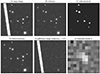 |
Fig. 1. Illustration of the difference-imaging process using a 65″ stamp of Pan-STARRS data. Panel A shows an image obtained at any given epoch (I(x) in the text or target image), and panel B shows the best-seeing image of the time series, i.e. the reference image. Panel C shows the pixels that are used in the least-squares procedure. Saturated pixels are not considered. The blurred reference image is show in panel D, and panel E shows the residuals after the blurred reference is subtracted from the target image. The kernel used to blur the reference image is shown in panel F. In the present case, it is simply a low-pass filter coupled to a small translation accounting for the shift between the target and reference images. |
2.3. Tests with Pan-STARRS data
We performed two types of tests of the method on real data. First, we applied it to known lensed quasars. Starting from the 191 lensed quasars in Lemon et al. (2019) that fall in the Pan-STARRS footprint, we find that 133 show extended variability. This is an encouraging performance, even though 34 of the variability maps were not reliable due to the high brightness of the targets themselves. In these cases, the transition kernel K was not properly constrained from the fainter stars in the field, causing a poor subtraction of the PSFs of the candidate and leaving non-PSF-like residuals. This experiment allowed us to set the reliability threshold of our method at a Gaia G-mag of 17, given the magnitude distribution of PSF stars available in practice.
Second, we examined the case of apparent quasar+star pairs, which are the most common contaminants to lens searches. Fortunately, the fraction of variable quasars is much higher than the fraction of variable stars because the majority of quasars tend to vary by more than 0.1 mag over two years (Cimatti et al. 1993). To benchmark the correct rejection of stars, we built a small selection of quasar+star systems by cross-matching the MILLIQUAS (Flesch 2021) and Gaia EDR3 (Gaia Collaboration 2021) catalogues and imposing additional restrictions: We requested that the proper motion significance (PMSIG; see Lemon et al. 2019 for the definition) of the companion be high enough to ensure that we did not include another quasar, and a small Gaia G-magnitude difference between the two. Ideally, the resulting systems should all produce variability in which one PSF is visible at most. This was achieved for 164 of the 170 test systems. Of the remaining 6 systems, 3 lack sufficient Pan-STARRS coverage for difference imaging, and the difference imaging performs poorly for the other 3 systems because too few reference stars are available even when we used large cutouts. In these cases, the variability maps incorrectly show variability. This shows that the method is able to efficiently reject quasar+star pairs, although care must still be taken to assess the quality of the difference imaging.
3. Candidate selection
To maximise the chances of lens discovery, we first built a catalogue of sources that were likely to contain a quasar. To do this, we combined the Gaia (Gaia Collaboration 2018) and WISE (Wright et al. 2010) catalogues. We started with all the WISE detections that were red enough, that is, whose WISE colour fulfilled

This criterion is stricter than that used by Lemon et al. (2019), but it helps to reduce the number of candidates to a manageable number for this proof of concept at the cost of losing bluer candidates. Then, we selected from the red WISE detections only those with a first Gaia detection within 3″ and a second Gaia detection between 0.8″ and 3″ away from the first detection. All the detections with a PMSIG larger than 3 are discarded. We also eliminated all the detections within 15° of the Galactic plane to reduce the likelihood of selecting stars. With these criteria, our final selection consisted of 14 591 objects, including 43 known lenses.
Next, we used all the available Pan-STARRS cutouts in the r and i band of the objects selected above. The choice of the r band was motivated by the fact that quasars are more variable in bluer bands (e.g. MacLeod et al. 2010), but the g band typically comes with harder-to-model PSFs. The i band was also included to patch the regions in which the r band was not available. We were unable to analyse 484 candidates because the data were insufficient: fewer than two epochs were available for these candidates. Consequently, a total of 14 107 variability maps were generated using our difference-imaging method. Out of these, 9692 maps were discarded due to the absence of any discernible signal above the background noise level. This left 4415 maps requiring visual inspection. We excluded 3300 more that showed a single PSF-like structure in the variability maps, but no extended variability. For the remaining maps displaying extended variation, we ensured that the stars in the rest of the field were indeed properly subtracted. This was not the case for 720 more maps, in which the difference-imaging procedure failed. This is usually caused by a lack of stars that are bright enough in the field, leading to a poor constraint of the transition kernel K, or other defects (see Appendix A.6). Lastly, we inspected the Pan-STARRS gri colour stamps of each candidate, giving priority to those showing consistent colour across PSFs. We excluded 166 more objects that clearly did not look like lenses. Ultimately, we identified a total of 229 variable objects, including 20 known lenses. From this subset, we further narrowed down our selection to 14 particularly promising candidates for spectroscopic follow-up. We also recovered 21 of the 43 known lenses in the preselection: This incompleteness is in part a result of our visual inspection, which favoured purity through the preferential selection of weaker objects with perfectly achieved difference imaging.
4. Follow-up observations and results
4.1. Spectroscopy
Eight systems were observed with grism 13 with the ESO Faint Object Spectrograph and Camera 2 (EFOSC2) on the ESO New Technology Telescope (NTT) over two runs in October 2020 and January 20213, providing a dispersion of 2.77 Å per pixel. Each object received between 900 and 1200 s of exposure time. Four other systems were observed with grism 4 and the Alhambra Faint Object Spectrograph and Camera (ALFOSC) on the Nordic Optical Telescope (NOT) in April 20214, providing a dispersion of 3.3 Å per pixel. Each object received between 900 and 1200 s of exposure time.
The general spectral reduction was carried out exactly as described in Lemon et al. (2023). The key steps are as follows. Each two-dimensional long-slit spectrum image is bias-subtracted, and cosmic rays are masked using a Laplacian threshold method. The threshold is adjusted based on the brightness of the objects and a visual inspection of the cosmic-ray mask. Next, the sky background is subtracted at each wavelength by determining the median value within the pixels surrounding the object trace, providing a sky-subtracted, debiased, cosmic-ray-masked two-dimensional long-slit spectrum image. A corresponding two-dimensional noise map is then generated, combining a Poisson noise map derived from the detector gain with the sky noise. Finally, a wavelength solution is established by fitting lines from a pre-observation arc exposure (HeNe or CuAr), and linearly shifted for each exposure to fit several major sky background emission lines. At each wavelength, a model of the 1D spatial profile of the two components is generated as two Moffat profiles separated by the Gaia separation, and integrated perpendicularly in the slit. The Moffat parameters as a function of wavelength are then determined by fitting this model to several bins across the wavelength. Finally, the flux of each component can be derived at each wavelength by using the best-fit Moffat parameters at each wavelength.
4.2. Imaging
The Pan-STARRS data are limited in depth when any potential lens galaxy between the quasar pairs is to be detected. Because of the narrow separations and faint magnitudes of our candidates, we obtained deeper images of the seven southern double-type candidates in the Rc band using the Wide Field Imager (WFI) on the Max-Planck-Institut für Astrophysik (MPIA) 2.2-m telescope (2p2) in nights of excellent seeing between March and June 2022. We obtained a total exposure time of 4 × 320 s per target.
Due to the complex PSF in these new images, we built a PSF model oversampled by a factor of 3, using up to six stars in each field. Next, we performed a joint deconvolution for each object, fitting the positions and amplitudes of two point sources as well as a Starlet-regularised pixelated background. Because galaxies are known to be sparse in Starlet space, we expect the lensing galaxy to naturally emerge in the background if it is detectable in the dataset. We used STARRED (Michalewicz et al. 2023) to perform both the PSF modelling and the image deconvolution.
When deeper Legacy Survey data or Hyper Suprime-Cam Subaru Strategic Program (HSC, Aihara et al. 2022) data were available, we performed a similar analysis, but replaced the pixelated background with an analytical Sérsic (Sérsic 1963) profile. The Legacy Survey and Pan-STARRS data were then fit jointly, but the HSC images were analysed on their own because their signal-to-noise ratio is vastly superior. We also make the code publicly available that we developed for this analysis5.
4.3. Discussion: Quasar pairs
Figure 3 shows the Pan-STARRS gri stacks and variability maps of all the double-type candidates for which we have follow-up imaging, ordered by right ascension. The variability of PS J0125−1012 clearly shows an artefact in one of the cutouts, but we still selected it given the general look of the Pan-STARRS gri cutout. We show the acquired spectra in Fig. 4. Eight of the 12 double-type candidates are spectroscopic quasar pairs (similar spectra in both components), one is a projected quasar pair, 2 are quasar+star pairs, and one is a pair of stars. Below, we tentatively classify the spectroscopic quasar pairs with comments referring to the spectra of Fig. 4, the 2p2 images of Fig. 2, and the available survey data of Fig. 5.
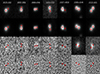 |
Fig. 2. MPIA 2.2-m telescope Rc-band data and models of the candidates visible from La Silla Observatory. First row: Stacked exposures (4 × 320 s). Second row: Modelling of the systems using the STARRED algorithm. Third row: Residuals after subtractions of the point-source component of the STARRED model. Last row: Residuals after subtraction of the complete STARRED model (PSFs + background). Each row shows a stack, but the data were deconvolved jointly. The red crosses indicate the positions of the PSFs, the separations of which are close to the Gaia separations down to 0.01″ (Table 1). At this depth and filter, the lensing galaxy is well detectable in only the two brightest objects. We provide the deconvolution-obtained magnitudes of this 2p2 data in Appendix B. |
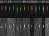 |
Fig. 3. Pan-STARRS Lupton-stretched (Lupton et al. 2004) gri views (top) and r+i variability maps (bottom) of the candidates selected for spectroscopic follow-up. Extended variability is still well visible for all the candidates, even though it sometimes barely rises above the noise. Candidates that are found to be false positives are displayed in grey, and the quasar pairs are displayed in white. The variability map of PS J0125−1012 includes an artefact. |
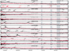 |
Fig. 4. Long-slit spectroscopy of double-type candidates performed using EFOSC2 on the ESO/NTT or ALFOSC on the Nordic Optical Telescope. The candidates are arranged in ascending order of right ascension, with lenses or quasar pairs written in bold and stars or projected quasars in grey. The shaded regions indicate wavelength ranges that are affected by atmospheric absorption. The spectra were reliably deblended using the procedure outlined in Sect. 4.1. The flux ratios of the quasar pairs can be found in Fig. C.1. |
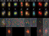 |
Fig. 5. Selection of the best-quality survey data and the modelling of these data. First row: Legacy Survey, Pan-STARRS (italicised), or HSC (bold) data. Second row: Models with 2 PSFs and an additional Sérsic profile when it significantly improves the modelling. Third row: Residuals after subtraction of the models. Fourth row: When the model has a Sérsic profile, residuals after subtraction of the PSFs alone. The bands are arranged by wavelength (redder first) and Lupton-stretched, highlighting the redder hue of the lensing galaxies seen in the fourth row compared to the quasar pairs. |
PS J0125−1012. The NTT/EFOSC2 resolved spectrum shows two quasars at redshift z = 1.22 with very similar continua and broad emission lines. We jointly fit the iz Legacy Survey and rzy Pan-STARRS bands. The data were well modelled with only two point sources, and the resulting image separation is 1.12″, compatible with the Gaia measurement. Although the reduced χ2 of the fit can be slightly improved by allowing for an additional Sersic profile, the improvement is not significant and the point sources are pushed further apart, breaking the compatibility with the Gaia separation. The similar 50 OM10 mock doubles, that is, those with source redshifts within Δz = 0.1 and image separations within 0.1″, their faintest lens galaxy magnitudes are i ∼ 21.1. This should be detectable at the depth of our Legacy Survey + Pan-STARRS cutouts. If this system is indeed a dual quasar, the physical separation would be 9.3 kpc. We suggest that this system is a dual quasar, but designate it as an unclassified quasar pair (UQP) until deeper high-resolution imaging can be obtained.
PS J0557−2959. The NTT/EFOSC2 resolved spectrum shows two quasars at redshift z = 2.04 with identical continua and broad emission lines. Even though our shallower r-band 2p2 data are well fit with two PSFs, the same fit of Legacy Survey data shows a clear sign of a lensing galaxy in the z-band data. This residual subsequently disappears when a Sérsic profile is included, which falls between the quasars. We also note that the PSF separation is 0.783″ when fitting without a galaxy, and 0.808″ when fitting with a galaxy, the latter of which agrees better with the Gaia separation of 0.810″, providing more evidence for the existence of the lensing galaxy. We therefore conclude that this system is a lensed quasar.
PS J0909−0749. The NTT/EFOSC2 resolved spectrum shows two quasars at redshift z = 1.08 with distinct differences in the ratio of the continuum and broad lines. There is no evidence for a lensing galaxy in the WFI 2p2 imaging. The simultaneous fit of Legacy Survey iz and Pan-STARRS grizy data with two point sources is good and does not significantly improve when a Sérsic profile is added. The Gaia separation is also recovered without the need for a model containing a galaxy. Moreover, the 38 similar OM10 mocks can have galaxies as faint as i ∼ 21.2, which should be detectable. Because of the slight differences in spectra and the lack of a lensing galaxy, we suggest that this system is a dual quasar with a physical separation 6.6 kpc. However, we conservatively designate this system as an UQP that needs deeper high-resolution imaging.
PS J1019−1322. The NTT/EFOSC2 resolved spectrum shows two quasars at redshift z = 2.32 with very similar shapes of the emission line profile. The flux ratio across the wavelength is ∼2.2, with some small variations around the emission lines. There is no evidence for a lensing galaxy in the WFI 2p2 imaging. Similarly, the simultaneous fit of the Pan-STARRS grizy and Legacy Survey griz data with two point sources does not leave significant residuals, and the Gaia separation is recovered as well. Similar mocks from the OM10 catalogue can have galaxy magnitudes as faint as i ∼ 22.6. We suggest that this system is a lensed quasar because of the similarity of the spectra, but a deep image detecting the lensing galaxy is still needed. We designate this system as an UQP.
PS J1037+0018. The NTT/EFOSC2 resolved spectrum shows two very similar quasars at redshift z = 2.46. The flux ratio is approximately 5.5 across all wavelengths, and both spectra show a damped Lyman-alpha system. The available HSC images are poorly fit with two point sources, but the subsequent introduction of a Sérsic profile produces much cleaner residuals. A subtraction of the two point sources then reveals the lensing galaxy close to the fainter point source. Moreover, the HSC images available here have a sufficient depth to produce a STARRED deconvolution of reliable appearance, which we show in Fig. 6. Based on all this evidence, we designate this system as a lens.
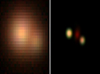 |
Fig. 6. HSC image of PS J1037+0018 and its STARRED deconvolution, both gry Lupton-stretched composites. The lens galaxy is well visible in the starlet-regularised background. Note the consistency of the fitted galaxy and point sources astrometry across filters. The measured magnitudes are given in Appendix B. |
PS J1225+4831. This system has also been discovered by Yue et al. (2023), who obtained Large Binocular Telescope LUCI1 imaging with an effective PSF of 0.35″ (FWHM). The images show no evidence for a lensing galaxy, and the authors further noted a possible flux ratio difference between the Hβ and [O III] lines. We present resolved NTT/EFOSC2 spectra of the system, which show two quasars at redshift z = 3.09 with a reasonably constant flux ratio of 3 across wavelength. Similar systems in the OM10 mock catalogue have lensing galaxies as faint as i ∼ 23.7. One possible explanation of these observations is that the lensing galaxy falls very close to one of the images and is being fit by the PSF subtraction of Yue et al. (2023), and the spectrum of the fainter component is too noisy to conclude incompatibility with the spectrum of the brighter object. Additionally, jointly fitting the available Pan-STARRS and Legacy Survey data produces slightly prominent residuals with a 2-PSF model, but the colour of these residuals matches that of the point sources. We thus attribute the poor fit to a defect in our PSF model, and thereby cannot find evidence for a lensing galaxy either. If this system were a dual quasar, its physical separation would be 6.87 kpc. We designate this system as an UQP, needing deeper imaging to confirm the presence or absence of the lensing galaxy.
PS J1800+0146. The NOT/ALFOSC resolved spectrum shows two very similar quasars at redshift z = 1.53. The flux ratio is roughly one across wavelength. Here, the 116 similar OM10 mocks suggest a lensing galaxy as faint as i ∼ 21.6 that is relatively bright and was blindly picked up by starlets in the 2p2 data. Fitting jointly the g and y Pan-STARRS images leaves residuals that disappear upon addition of a Sérsic profile. The Gaia separation of 1.12″ is also recovered by both 2p2 and Pan-STARRS fits. We designate this system as a lens.
PS J2122−1621. The NTT/EFOSC2 resolved spectrum shows two very similar quasars at redshift z = 1.47, with a flux ratio of ∼1.2 across the wavelength. Just like the case of PS J1800+0146, the lensing galaxy could be fitted blindly with STARRED in the 2p2 data. Moreover, even if the Pan-STARRS data can be modelled with two point sources alone, the separation is then underestimated by 0.05″. The addition of a Sérsic profile again recovers the Gaia separation. We designate this system as a lens.
Table 1 summarizes the outcome of the discussions for each candidate.
Confirmed quasar pairs. We show the separation between the two images from Gaia, the spectroscopic redshift, and the Gaia G magnitudes.
5. Conclusions
Our search using difference imaging in Pan-STARRS led to the identification of four new doubly lensed quasars and four UQPs that are either lenses or dual quasars, and one projected quasar pair. Notably, all of the lenses have a narrow separation between 0.81″ and 1.24″, and three have source redshifts above z = 1.5. This distribution is thereby starting to fill the gap pointed out by Lemon et al. (2023), where many small-separation high-redshift doubles are missing. Furthermore, Lemon et al. (2020) noted that there is a quad bias when variability is used to select lensed quasars, which can be understood by the fact that the more variable quasars are the least massive ones (MacLeod et al. 2010): They have fainter absolute magnitudes and would need to be highly magnified to reach a detectable threshold. This means that searching for lensed quasars through their variability introduces a high-magnification bias and is complementary to traditional search methods for the construction of a magnitude-limited lensed quasar catalogue. Because of the bias for strong magnification that our technique introduces, it may seem surprising that we do not find more quads. The reason is that all quads were already found at the Gaia limit (Lemon et al. 2019, 2023; Delchambre et al. 2019). As we extend the search to beyond the Gaia limit, we can expect that this time, quads will be detected at an increased rate.
In conclusion, we presented a difference-imaging technique and applied it to Pan-STARRS imaging with a Gaia+WISE preselection, focusing on detecting extended variability as an efficient method for the selection of lensed quasars. This work underlines the potential of extended variability and difference imaging as an effective method for the selection of lensed quasars, with great promise of uncovering highly magnified lenses in future surveys such as the forthcoming Vera Rubin Observatory’s Legacy Survey of Space and Time (Ivezić et al. 2019, LSST). When we consider the anticipated scarcity of spectroscopic resources in the future relative to the vast number of candidates expected to be uncovered by LSST, attaining a high level of purity in candidate selection through their variability will become increasingly important.
From a compilation of the literature, see also Lemon et al. (2020).
Timo Anguita, 106.218K.001 and 106.218K.002.
Cameron Lemon, 63-106.
Acknowledgments
This program is supported by the Swiss National Science Foundation (SNSF) and by the European Research Council (ERC) under the European Union’s Horizon 2020 research and innovation program (COSMICLENS: grant agreement No. 787886). T.A. acknowledges support from the Millennium Science Initiative ICN12_009 and the ANID BASAL project FB210003. 2p2: The 2p2 imaging was made possible by an agreement between MPIA and EPFL, the ESO program ID is 0108.A-9005(A). Pan-STARRS: The Pan-STARRS1 Surveys (PS1) and the PS1 public science archive have been made possible through contributions by the Institute for Astronomy, the University of Hawaii, the Pan-STARRS Project Office, the Max-Planck Society and its participating institutes, the Max Planck Institute for Astronomy, Heidelberg and the Max Planck Institute for Extraterrestrial Physics, Garching, The Johns Hopkins University, Durham University, the University of Edinburgh, the Queen’s University Belfast, the Harvard-Smithsonian Center for Astrophysics, the Las Cumbres Observatory Global Telescope Network Incorporated, the National Central University of Taiwan, the Space Telescope Science Institute, the National Aeronautics and Space Administration under Grant No. NNX08AR22G issued through the Planetary Science Division of the NASA Science Mission Directorate, the National Science Foundation Grant No. AST-1238877, the University of Maryland, Eotvos Lorand University (ELTE), the Los Alamos National Laboratory, and the Gordon and Betty Moore Foundation. HSC: The Hyper Suprime-Cam (HSC) collaboration includes the astronomical communities of Japan and Taiwan, and Princeton University. The HSC instrumentation and software were developed by the National Astronomical Observatory of Japan (NAOJ), the Kavli Institute for the Physics and Mathematics of the Universe (Kavli IPMU), the University of Tokyo, the High Energy Accelerator Research Organization (KEK), the Academia Sinica Institute for Astronomy and Astrophysics in Taiwan (ASIAA), and Princeton University. Funding was contributed by the FIRST program from Japanese Cabinet Office, the Ministry of Education, Culture, Sports, Science and Technology (MEXT), the Japan Society for the Promotion of Science (JSPS), Japan Science and Technology Agency (JST), the Toray Science Foundation, NAOJ, Kavli IPMU, KEK, ASIAA, and Princeton University. Legacy Survey: The Legacy Surveys consist of three individual and complementary projects: the Dark Energy Camera Legacy Survey (DECaLS; Proposal ID #2014B-0404; PIs: David Schlegel and Arjun Dey), the Beijing-Arizona Sky Survey (BASS; NOAO Prop. ID #2015A-0801; PIs: Zhou Xu and Xiaohui Fan), and the Mayall z-band Legacy Survey (MzLS; Prop. ID #2016A-0453; PI: Arjun Dey). DECaLS, BASS and MzLS together include data obtained, respectively, at the Blanco telescope, Cerro Tololo Inter-American Observatory, NSF’s NOIRLab; the Bok telescope, Steward Observatory, University of Arizona; and the Mayall telescope, Kitt Peak National Observatory, NOIRLab. Pipeline processing and analyses of the data were supported by NOIRLab and the Lawrence Berkeley National Laboratory (LBNL). The Legacy Surveys project is honored to be permitted to conduct astronomical research on Iolkam Du’ag (Kitt Peak), a mountain with particular significance to the Tohono O’odham Nation. NOIRLab is operated by the Association of Universities for Research in Astronomy (AURA) under a cooperative agreement with the National Science Foundation. LBNL is managed by the Regents of the University of California under contract to the US Department of Energy. This project used data obtained with the Dark Energy Camera (DECam), which was constructed by the Dark Energy Survey (DES) collaboration. Funding for the DES Projects has been provided by the US Department of Energy, the US National Science Foundation, the Ministry of Science and Education of Spain, the Science and Technology Facilities Council of the United Kingdom, the Higher Education Funding Council for England, the National Center for Supercomputing Applications at the University of Illinois at Urbana-Champaign, the Kavli Institute of Cosmological Physics at the University of Chicago, Center for Cosmology and Astro-Particle Physics at the Ohio State University, the Mitchell Institute for Fundamental Physics and Astronomy at Texas A&M University, Financiadora de Estudos e Projetos, Fundacao Carlos Chagas Filho de Amparo, Financiadora de Estudos e Projetos, Fundacao Carlos Chagas Filho de Amparo a Pesquisa do Estado do Rio de Janeiro, Conselho Nacional de Desenvolvimento Cientifico e Tecnologico and the Ministerio da Ciencia, Tecnologia e Inovacao, the Deutsche Forschungsgemeinschaft and the Collaborating Institutions in the Dark Energy Survey. The Collaborating Institutions are Argonne National Laboratory, the University of California at Santa Cruz, the University of Cambridge, Centro de Investigaciones Energeticas, Medioambientales y Tecnologicas-Madrid, the University of Chicago, University College London, the DES-Brazil Consortium, the University of Edinburgh, the Eidgenossische Technische Hochschule (ETH) Zurich, Fermi National Accelerator Laboratory, the University of Illinois at Urbana-Champaign, the Institut de Ciencies de l’Espai (IEEC/CSIC), the Institut de Fisica d’Altes Energies, Lawrence Berkeley National Laboratory, the Ludwig Maximilians Universitat Munchen and the associated Excellence Cluster Universe, the University of Michigan, NSF’s NOIRLab, the University of Nottingham, the Ohio State University, the University of Pennsylvania, the University of Portsmouth, SLAC National Accelerator Laboratory, Stanford University, the University of Sussex, and Texas A&M University. BASS is a key project of the Telescope Access Program (TAP), which has been funded by the National Astronomical Observatories of China, the Chinese Academy of Sciences (the Strategic Priority Research Program “The Emergence of Cosmological Structures” Grant # XDB09000000), and the Special Fund for Astronomy from the Ministry of Finance. The BASS is also supported by the External Cooperation Program of Chinese Academy of Sciences (Grant # 114A11KYSB20160057), and Chinese National Natural Science Foundation (Grant # 12120101003, # 11433005). The Legacy Survey team makes use of data products from the Near-Earth Object Wide-field Infrared Survey Explorer (NEOWISE), which is a project of the Jet Propulsion Laboratory/California Institute of Technology. NEOWISE is funded by the National Aeronautics and Space Administration. The Legacy Surveys imaging of the DESI footprint is supported by the Director, Office of Science, Office of High Energy Physics of the US Department of Energy under Contract No. DE-AC02-05CH1123, by the National Energy Research Scientific Computing Center, a DOE Office of Science User Facility under the same contract; and by the US National Science Foundation, Division of Astronomical Sciences under Contract No. AST-0950945 to NOAO.
References
- Aihara, H., AlSayyad, Y., Ando, M., et al. 2022, PASJ, 74, 247 [NASA ADS] [CrossRef] [Google Scholar]
- Alard, C., & Lupton, R. H. 1998, ApJ, 503, 325 [Google Scholar]
- Bertin, E., & Arnouts, S. 1996, A&AS, 117, 393 [NASA ADS] [CrossRef] [EDP Sciences] [Google Scholar]
- Blanton, M. R., & Roweis, S. 2007, AJ, 133, 734 [NASA ADS] [CrossRef] [Google Scholar]
- Bramich, D. M. 2008, MNRAS, 386, L77 [NASA ADS] [CrossRef] [Google Scholar]
- Bramich, D. M., Horne, K., Albrow, M. D., et al. 2012, MNRAS, 428, 2275 [Google Scholar]
- Chambers, K. C., Magnier, E. A., Metcalfe, N., et al. 2016, ArXiv e-prints [arXiv:1612.05560] [Google Scholar]
- Chan, J. H. H., Lemon, C., Courbin, F., et al. 2022, A&A, 659, A140 [NASA ADS] [CrossRef] [EDP Sciences] [Google Scholar]
- Chao, D. C. Y., Chan, J. H. H., Suyu, S. H., et al. 2020, A&A, 640, A88 [NASA ADS] [CrossRef] [EDP Sciences] [Google Scholar]
- Chao, D. C. Y., Chan, J. H. H., Suyu, S. H., et al. 2021, A&A, 655, A114 [NASA ADS] [CrossRef] [EDP Sciences] [Google Scholar]
- Cimatti, A., Zamorani, G., & Marano, B. 1993, MNRAS, 263, 236 [NASA ADS] [CrossRef] [Google Scholar]
- Delchambre, L., Krone-Martins, A., Wertz, O., et al. 2019, A&A, 622, A165 [NASA ADS] [CrossRef] [EDP Sciences] [Google Scholar]
- Flesch, E. W. 2021, ArXiv e-prints [arXiv:2105.12985] [Google Scholar]
- Gaia Collaboration (Brown, A. G. A., et al.) 2018, A&A, 616, A1 [NASA ADS] [CrossRef] [EDP Sciences] [Google Scholar]
- Gaia Collaboration (Brown, A. G. A., et al.) 2021, A&A, 649, A1 [NASA ADS] [CrossRef] [EDP Sciences] [Google Scholar]
- Ivezić, Ž., Kahn, S. M., Tyson, J. A., et al. 2019, ApJ, 873, 111 [Google Scholar]
- Kochanek, C. S., Mochejska, B., Morgan, N. D., & Stanek, K. Z. 2006, ApJ, 637, L73 [NASA ADS] [CrossRef] [Google Scholar]
- Kormendy, J., Fisher, D. B., Cornell, M. E., & Bender, R. 2009, ApJS, 182, 216 [Google Scholar]
- Kostrzewa-Rutkowska, Z., Kozłowski, S., Lemon, C., et al. 2018, MNRAS, 476, 663 [NASA ADS] [CrossRef] [Google Scholar]
- Lacki, B. C., Kochanek, C. S., Stanek, K. Z., Inada, N., & Oguri, M. 2009, ApJ, 698, 428 [NASA ADS] [CrossRef] [Google Scholar]
- Lemon, C. A., Auger, M. W., & McMahon, R. G. 2019, MNRAS, 483, 4242 [NASA ADS] [CrossRef] [Google Scholar]
- Lemon, C., Auger, M. W., McMahon, R., et al. 2020, MNRAS, 494, 3491 [NASA ADS] [CrossRef] [Google Scholar]
- Lemon, C., Anguita, T., Auger-Williams, M. W., et al. 2023, MNRAS, 520, 3305 [NASA ADS] [CrossRef] [Google Scholar]
- Lupton, R., Blanton, M. R., Fekete, G., et al. 2004, PASP, 116, 133 [NASA ADS] [CrossRef] [Google Scholar]
- MacLeod, C. L., Ivezić, Ž., Kochanek, C. S., et al. 2010, ApJ, 721, 1014 [Google Scholar]
- Magnier, E. A., Schlafly, E., Finkbeiner, D., et al. 2013, ApJS, 205, 20 [Google Scholar]
- Michalewicz, K., Millon, M., Dux, F., & Courbin, F. 2023, J. Open Source Softw., 8, 5340 [NASA ADS] [CrossRef] [Google Scholar]
- Mingarelli, C. M. F. 2019, Nat. Astron., 3, 8 [CrossRef] [Google Scholar]
- Oguri, M., & Marshall, P. J. 2010, MNRAS, 405, 2579 [NASA ADS] [Google Scholar]
- Refsdal, S. 1964, MNRAS, 128, 307 [NASA ADS] [CrossRef] [Google Scholar]
- Sérsic, J. L. 1963, Boletin de la Asociacion Argentina de Astronomia La Plata Argentina, 6, 41 [Google Scholar]
- Shajib, A. J., Birrer, S., Treu, T., et al. 2020, MNRAS, 494, 6072 [Google Scholar]
- Treu, T., Agnello, A., Baumer, M. A., et al. 2018, MNRAS, 481, 1041 [NASA ADS] [CrossRef] [Google Scholar]
- Udalski, A., Szymanski, M., Kaluzny, J., Kubiak, M., & Mateo, M. 1992, Acta Astron., 42, 253 [NASA ADS] [Google Scholar]
- Verde, L., Treu, T., & Riess, A. G. 2019, Nat. Astron., 3, 891 [Google Scholar]
- Waters, C. Z., Magnier, E. A., Price, P. A., et al. 2020, ApJS, 251, 4 [NASA ADS] [CrossRef] [Google Scholar]
- Wong, K. C., Suyu, S. H., Chen, G. C. F., et al. 2020, MNRAS, 498, 1420 [Google Scholar]
- Wright, E. L., Eisenhardt, P. R. M., Mainzer, A. K., et al. 2010, AJ, 140, 1868 [Google Scholar]
- Yue, M., Fan, X., Yang, J., & Wang, F. 2023, AJ, 165, 191 [NASA ADS] [CrossRef] [Google Scholar]
Appendix A: Technical details of the difference imaging
A.1. Choice of the reference image
It would be optimal for the transition kernel to be a low-pass filter. In the opposite case, the reference image is convoluted with a high-pass filter, which equates a deconvolution. This is not necessarily undesired because the operation is still photometric, but it will create ringing artefacts and instabilities. When possible, the reference image is therefore chosen to be the one with the best seeing, such that it needs to be blurred to be adapted onto the other images of the set. Because of the nature of Pan-STARRS data, however, this is not always possible: When a large portion of the best-seeing image is missing (see Section A.2), two or more images (in order of ascending seeing) are combined to provide enough reference stars because too few eligible pixels for the matching procedure decreases the condition number of the matrix of Eq. (4), leading to more numerical instability.
A.2. Masking bad and irrelevant pixels
The matrix in Eq. (4) can become very large, making the least-squares problem slower to solve. The complexity of this step is roughly ∼𝒪(N4(n + N2)). N is defined by the size of the kernel, but n can be advantageously reduced. Most of the pixels in an astronomical image are dark and do not carry information. Worse, the brightest stars in a field are usually burnt, contribute much to the χ2 due to their high intensity and do not contain valid information about the PSF. The first step is therefore to mask the background and the very bright pixels. These were identified using sextractor (Bertin & Arnouts 1996), which can produce segmentation maps that label each star and the background, together with the output catalogue of stars that links each label in the segmentation map with a magnitude. All stars brighter than a magnitude threshold are masked.
Next comes the Pan-STARRS specific masking: Pan-STARRS cutouts come with useful auxiliary data such as noise maps (used for the weighting of the pixels in the χ2 minimisation) and masks. The latter contain flags labelling each pixel with one of the 17 ways (as defined by Pan-STARRS) in which a pixel can be bad. Fig. A.1 shows a typical cutout where empty, dead, or burnt pixels are visible. We only selected the pixels that were flag-free. Overall, masking decreases n by up to three orders of magnitude and substantially increases the robustness of the algorithm.
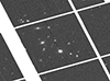 |
Fig. A.1. Typical cutout as delivered by the Pan-STARRS cutout server. The size of this field is 256″ × 256″ (1024 × 1024 pixels2). Throughout this work, we mostly used 128″ × 128″ cutouts, but allowed for the possibility of increasing the size of the field when we failed to find useful stars that were able to constrain the transition kernel. |
A.3. Noise map of a difference image
When blurring the reference image, in particular, as in Eq. (3), the transition kernel Kj was chosen in the sense of the least squares of the sum of Eq. (2) so as to blur the reference R(x) to match the resolution of the target image I(x). However, the weights  do not constitute a good noise map for the resulting difference image ΔI(x) = Rblurred(x)−I(x). The latter is the sum of PSF-matched images, whereas the former combines two different resolutions. As a first-order correction, we blurred
  ) with the optimised kernel Kj,
 (A.1)
(A.1)
where including the background B would not make sense because the variance is translation invariant. Then, the final noise map is
 (A.2)
(A.2)
After the algorithm completes, a new value of reduced χ2 is calculated using the corrected noise map (A.2) and is later used to select the best difference images. With this correction, the reduced χ2 value averages roughly one for kernel sizes from 7×7 to 13×13 pixels2.
A.4. Choice of the contributing difference images
When building variability maps, we need to maximise the chance that some variability is observed. We therefore enforced that exactly one difference image per available night of observation was chosen. Of the available images in each night, we chose the image that best covered the central region. If all of them offered a decent covering, we selected the image with the best seeing value. The difference images whose generation procedure failed (reduced χ2 over some threshold) were not candidates to this heuristic of the selection.
A.5. Kernel extent and overfitting
Matching two images with a large difference in their PSF requires a transfer kernel with a large spatial extent. In this implementation, extending the kernel by a factor Q increases the number of degrees of freedom in the fits Q2 folds. This often led to reduced χ2 values much smaller than 1, suggesting that the fit could be carried out meaningfully and faster with fewer degrees of freedom. In the present context, the process was unfolding fast enough and no further optimisation was undertaken. When working with very large images, however, one might want to implement the multi-resolution approach developed by Bramich et al. (2012). In this paradigm, the outer pixels of the kernel are binned to increase the spatial extent of the kernel without quadratically increasing the number of degrees of freedom.
A.6. Examples of corrupted variability maps
The proper classification of the variability maps posed a challenge because the maps can be corrupt in numerous ways. A few examples, both bad and good, are listed in Fig. A.2. The difference imaging sometimes simply fails even when the reduced χ2 values are in an acceptable range. This can arise, for example, when the candidate is much brighter than any of the stars in the field. The structure of the PSF is then under-determined, and the transition kernel will only guarantee the proper subtraction of sources near the noise level. This will also happen with meteors or satellites, or in the rarer case when one of the cutouts is not properly aligned with the others.
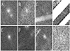 |
Fig. A.2. Different crops of variability maps and problems. A: A valid detection. B: One of the original images had normalisation problems. C: CCD bleeding in one of the original images because of a very bright star. D: Heavily banded region, missing data. E: Valid image, but only one variable patch. F: The original images contain a very bright star that cannot be properly subtracted at the edge. G: An uncaught cosmic. H: Valid image, no variability. |
Appendix B: Magnitudes from deconvolutions
In Table B.1 we give the Vega magnitude measurements from the fully fledged STARRED deconvolutions performed in this work. The zero-points of the 2p2 data were determined approximately using the Pan-STARRS r filter (which has a large overlap with the ESO Rc filter) stars. The HSC magnitudes were approximately converted from AB into Vega using the filter transformations from Blanton & Roweis (2007). The quoted uncertainties only include the statistical component of the fit and zero-point determination dispersion.
Vega magnitudes obtained from STARRED deconvolutions.
Appendix C: Spectral ratios
To highlight where the spectral differences might be important, we provide the ratios of the spectra presented in Fig. 4. The ratios are shown in Fig. C.1.
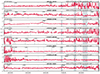 |
Fig. C.1. Flux ratios of the spectra of the quasar pairs presented in Fig. 4. The ratios were smoothed with an 8 Å wide (FWHM) Gaussian kernel for clarity. |
All Tables
Confirmed quasar pairs. We show the separation between the two images from Gaia, the spectroscopic redshift, and the Gaia G magnitudes.
All Figures
|
Fig. 1. Illustration of the difference-imaging process using a 65″ stamp of Pan-STARRS data. Panel A shows an image obtained at any given epoch (I(x) in the text or target image), and panel B shows the best-seeing image of the time series, i.e. the reference image. Panel C shows the pixels that are used in the least-squares procedure. Saturated pixels are not considered. The blurred reference image is show in panel D, and panel E shows the residuals after the blurred reference is subtracted from the target image. The kernel used to blur the reference image is shown in panel F. In the present case, it is simply a low-pass filter coupled to a small translation accounting for the shift between the target and reference images. |
| In the text | |
|
Fig. 2. MPIA 2.2-m telescope Rc-band data and models of the candidates visible from La Silla Observatory. First row: Stacked exposures (4 × 320 s). Second row: Modelling of the systems using the STARRED algorithm. Third row: Residuals after subtractions of the point-source component of the STARRED model. Last row: Residuals after subtraction of the complete STARRED model (PSFs + background). Each row shows a stack, but the data were deconvolved jointly. The red crosses indicate the positions of the PSFs, the separations of which are close to the Gaia separations down to 0.01″ (Table 1). At this depth and filter, the lensing galaxy is well detectable in only the two brightest objects. We provide the deconvolution-obtained magnitudes of this 2p2 data in Appendix B. |
| In the text | |
|
Fig. 3. Pan-STARRS Lupton-stretched (Lupton et al. 2004) gri views (top) and r+i variability maps (bottom) of the candidates selected for spectroscopic follow-up. Extended variability is still well visible for all the candidates, even though it sometimes barely rises above the noise. Candidates that are found to be false positives are displayed in grey, and the quasar pairs are displayed in white. The variability map of PS J0125−1012 includes an artefact. |
| In the text | |
|
Fig. 4. Long-slit spectroscopy of double-type candidates performed using EFOSC2 on the ESO/NTT or ALFOSC on the Nordic Optical Telescope. The candidates are arranged in ascending order of right ascension, with lenses or quasar pairs written in bold and stars or projected quasars in grey. The shaded regions indicate wavelength ranges that are affected by atmospheric absorption. The spectra were reliably deblended using the procedure outlined in Sect. 4.1. The flux ratios of the quasar pairs can be found in Fig. C.1. |
| In the text | |
|
Fig. 5. Selection of the best-quality survey data and the modelling of these data. First row: Legacy Survey, Pan-STARRS (italicised), or HSC (bold) data. Second row: Models with 2 PSFs and an additional Sérsic profile when it significantly improves the modelling. Third row: Residuals after subtraction of the models. Fourth row: When the model has a Sérsic profile, residuals after subtraction of the PSFs alone. The bands are arranged by wavelength (redder first) and Lupton-stretched, highlighting the redder hue of the lensing galaxies seen in the fourth row compared to the quasar pairs. |
| In the text | |
|
Fig. 6. HSC image of PS J1037+0018 and its STARRED deconvolution, both gry Lupton-stretched composites. The lens galaxy is well visible in the starlet-regularised background. Note the consistency of the fitted galaxy and point sources astrometry across filters. The measured magnitudes are given in Appendix B. |
| In the text | |
|
Fig. A.1. Typical cutout as delivered by the Pan-STARRS cutout server. The size of this field is 256″ × 256″ (1024 × 1024 pixels2). Throughout this work, we mostly used 128″ × 128″ cutouts, but allowed for the possibility of increasing the size of the field when we failed to find useful stars that were able to constrain the transition kernel. |
| In the text | |
|
Fig. A.2. Different crops of variability maps and problems. A: A valid detection. B: One of the original images had normalisation problems. C: CCD bleeding in one of the original images because of a very bright star. D: Heavily banded region, missing data. E: Valid image, but only one variable patch. F: The original images contain a very bright star that cannot be properly subtracted at the edge. G: An uncaught cosmic. H: Valid image, no variability. |
| In the text | |
|
Fig. C.1. Flux ratios of the spectra of the quasar pairs presented in Fig. 4. The ratios were smoothed with an 8 Å wide (FWHM) Gaussian kernel for clarity. |
| In the text | |
Current usage metrics show cumulative count of Article Views (full-text article views including HTML views, PDF and ePub downloads, according to the available data) and Abstracts Views on Vision4Press platform.
Data correspond to usage on the plateform after 2015. The current usage metrics is available 48-96 hours after online publication and is updated daily on week days.
Initial download of the metrics may take a while.