| Issue |
A&A
Volume 682, February 2024
|
|
|---|---|---|
| Article Number | A83 | |
| Number of page(s) | 12 | |
| Section | Extragalactic astronomy | |
| DOI | https://doi.org/10.1051/0004-6361/202347394 | |
| Published online | 02 February 2024 | |
Nearby galaxies in the LOFAR Two-metre Sky Survey
III. Influence of cosmic-ray transport on the radio-SFR relation
1
Hamburg University, Hamburger Sternwarte, Gojenbergsweg 112, 21029 Hamburg, Germany
e-mail: This email address is being protected from spambots. You need JavaScript enabled to view it.
2
Ruhr University Bochum, Faculty of Physics and Astronomy, Astronomical Institute (AIRUB), 44780 Bochum, Germany
3
INAF – Istituto di Radioastronomia, Via Gobetti 101, 40129 Bologna, Italy
4
Aix-Marseille Univ., CNRS, CNES, LAM, Marseille, France
5
INAF – Padova Astronomical Observatory, Vicolo dell’Osservatorio 5, 35122 Padova, Italy
6
Università di Milano-Bicocca, Piazza della scienza 3, 20100 Milano, Italy
7
INAF – Osservatorio Astronomico di Brera, Via Brera 28, 20121 Milano, Italy
Received:
7
July
2023
Accepted:
20
September
2023
Abstract
Context. To understand galaxy evolution, it is essential to measure star formation rates (SFRs) across cosmic time.
Aims. The use of radio continuum emission as an extinction-free tracer of star formation necessitates a good understanding of the influence of cosmic-ray electron (CRE) transport. Our aim in this work is to improve this understanding.
Methods. We analysed the spatially resolved radio continuum-star formation rate (radio-SFR) relation in 15 nearby galaxies using data from the LOw Frequency ARray (LOFAR) and the Westerbork Synthesis Radio Telescope (WSRT) at 144 and 1365 MHz, respectively. The hybrid SFR maps are based on observations with Spitzer at 24 μm and with GALEX at 156 nm. Our pixel-by-pixel analysis at 1.2 kpc resolution reveals the usual sublinear radio-SFR relation for local measurements. This can be linearised with a smoothing experiment, convolving the hybrid SFR map with a Gaussian kernel that provides us with the CRE transport length.
Results. CRE transport can be described as energy-independent isotropic diffusion. If we consider only young CREs as identified with the radio spectral index, we find a linear relation showing the influence of cosmic-ray transport. We then define the CRE calorimetric efficiency as the ratio of radio-to-hybrid SFR surface density and show that it is a function of the radio spectral index. If we correct the radio-SFR relation for the CRE calorimetric efficiency parametrised by the radio spectral index, it becomes nearly linear with a slope of 1.01 ± 0.02, independent of frequency.
Conclusions. The corrected radio-SFR relation is universal and it holds for both global and local measurements.
Key words: cosmic rays / galaxies: fundamental parameters / galaxies: magnetic fields / galaxies: star formation / radio continuum: galaxies
© The Authors 2024
 Open Access article, published by EDP Sciences, under the terms of the Creative Commons Attribution License (https://creativecommons.org/licenses/by/4.0), which permits unrestricted use, distribution, and reproduction in any medium, provided the original work is properly cited.
This article is published in open access under the Subscribe to Open model. This email address is being protected from spambots. You need JavaScript enabled to view it. to support open access publication.
1. Introduction
Cosmic rays and magnetic fields are important components in our understanding of galaxy evolution. Both have energy densities comparable to the thermal gas and so influence the dynamics of gas accretion and outflows. Cosmic rays are now suspected to play an important role in galactic winds and the dynamics of the circumgalactic medium (e.g. Pakmor et al. 2020; van de Voort et al. 2021). Magnetic fields regulate the transport of cosmic rays and, thus, they need to be taken into account as well; however, they are crucial in their own right, as they also play an important role during the early stages of star formation by regulating the transport of angular momentum during the collapse of molecular clouds. The number density of cosmic rays can be approximated by a power law in electronvolts (eV) reaching from GeV above many orders of magnitude, although more recent works have shown deviations from this, particularly at energies in excess of PeV (see Gaisser et al. 2013, for a review). While cosmic rays may reach energies beyond even EeV, it is widely known that GeV-cosmic rays are dynamically the most important for gas motions, as they contain the bulk of the cosmic-ray energy density. We can observe these cosmic rays via their electron component the cosmic-ray electrons (CREs) and the same electrons emit synchrotron emission while spiralling around magnetic field lines, allowing us to observe them in the radio continuum.
Radio continuum emission is the result of massive star formation. Stars of the O and B spectral classifications ionise hydrogen in their environment forming Strömgren spheres. This ionised gas is visible in the radio continuum via free-free emission of electrons deflected in the electric field of protons; this radiation is referred to as thermal emission. At gigahertz (and lower) frequencies, the second emission process is even more important and dominates at fractions of > 90% in late-type galaxies (Tabatabaei et al. 2017; Stein et al. 2023). Massive stars end their relatively short lifes in core-collapse supernovae. In the aftermath of that explosion, strong shocks are formed that are able to accelerate cosmic rays in supernova remnants as predicted by theory (Drury 1983) and confirmed by observations (Aharonian et al. 2007). In addition to these primary cosmic rays, hadronically interacting cosmic-ray protons with ambient gas generate charged pions that decay into secondary electrons and positrons, which also radiate synchrotron emission. These cosmic rays are able to diffuse in galaxies, while emitting synchrotron radiation from their electrons; this radiation is referred to as non-thermal emission. In summary, the radio continuum luminosity of a galaxy should be proportional to the number of massive stars. This would allow us to derive the star formation rate (SFR) of a galaxy by extrapolating from the massive stars that must have been recently formed giving rise to the radio continuum-star formation rate (radio-SFR) relation (Condon 1992; Bell 2003; Murphy et al. 2011).
The radio-SFR relation has been extensively studied in galaxies (Boselli et al. 2015; Li et al. 2016; Davies et al. 2017; Tabatabaei et al. 2017; Gürkan et al. 2018; Hindson et al. 2018; Smith et al. 2021; Heesen et al. 2022). For integrated, global studies the slope of the relation appears to be slightly super-linear, so that galaxies with higher SFRs have radio luminosities, Lν, that are higher in comparison with their SFR. This appears to be particularly the case at lower frequencies of hundreds of megahertz with the relation Lν ∝ SFR1.4 − 1.5 observed, where the escape of CRE plays an important role due to the longer electron lifetimes (Heesen et al. 2022). In contrast, the spatially resolved radio-SFR relation is significantly sub-linear. This means that areas with low SFR surface densities are bright in the radio continuum emission, whereas the opposite is the case for areas with high SFR surface densities. This is usually ascribed to cosmic-ray transport as well, where the CREs diffuse away from star-forming areas into the galaxy outskirts and inter-arm regions (Berkhuijsen et al. 2013; Heesen et al. 2014). Indeed, the radio continuum map of a galaxy can be approximated as the smoothed out version of the SFR map where the size of the smoothing kernel can be associated with the CRE transport length (Vollmer et al. 2020; Heesen et al. 2023a).
In addition, it has emerged that the age of the CRE is an important secondary parameter. If we restrict the analysis of the radio-SFR relation to areas with high SFR surface densities, the relation in individual galaxies becomes almost linear (Dumas et al. 2011; Basu et al. 2012). Such a linear relation is predicted if the galaxy is an electron calorimeter and the CREs lose all their energy before being transported away. This means that the radio-SFR relation for young CRE found near their sources (i.e. star-forming regions) is not yet affected by cosmic-ray transport. Heesen & Buie (2019) found tentative evidence that the radio-SFR relation is universal and close to linear across several galaxies if we consider only areas with radio spectral indices indicative of young CRE. However, they considered only four galaxies limiting their applicability of conclusions. Hence, what is thus far missing is a study of the spatially resolved radio-SFR relation in a representative sample of nearby galaxies. This has now become possible with data from the LOFAR Two-metre Sky Survey (LoTSS; Shimwell et al. 2017, 2019, 2022). Heesen et al. (2022) defined a sample of 76 nearby galaxies in LoTSS that forms the basis of our analysis.
Our aim is to measure star formation rates in nearby galaxies using radio continuum emission. There are two main motivations behind this: first, the existence of a universal radio-SFR relation, both between galaxies and within galaxies implies a direct link between radio emissions and star formation. Second, if such a link was established it could be used to measure SFRs in galaxies of the local Universe (Beswick et al. 2015). The fact that radio emission is extinction-free as opposed to ultraviolet, H α, and partially also mid-infrared based methods would allow astronomers to measure star formation rates in high redshift galaxies. On the other hand, radio continuum-based methods could be impaired by inverse Compton losses that become more important at higher redshifts (Murphy 2009). The use of LOFAR is especially helpful in this context. At lower frequencies the thermal component of the radio emissions is even smaller with fractions below 5% (Stein et al. 2023). Lower frequencies also allow us to inspect lower energy CREs. Since the CREs travel significant distances (while emitting synchrotron radiation at the same time), the resulting radio map is a smeared out version of the true star formation distribution, with the effect being even more pronounced at lower frequencies (Heesen & Buie 2019).
There are broadly speaking three ways of measuring cosmic-ray transport parameters in nearby galaxies. First, one can compare the luminosity of a galaxy either in the radio continuum or in the gamma rays with the SFR. These correlations are slightly superlinear which can be interpreted that galaxies are better cosmic-ray calorimeters at higher masses and sizes (Ackermann et al. 2012; Li et al. 2016; Heesen et al. 2022). Second, one can use spectral analyses. If the spectrum is a continuous power-law in agreement with the injection spectrum, we can deduce that energy-independent transport such as by advection is the dominant transport. This is observed in some galaxies, both in gamma rays (Abramowski et al. 2012) as well as in the radio continuum (Kapińska et al. 2017). However, in the latter case, the interpretation is compounded by the effect of various energy losses that tend to flatten the spectrum at low energies via ionisation losses and steepen the spectrum at high energies via synchrotron and inverse Compton losses. Thirdly, one can compare the distribution of cosmic rays with the distribution of their sources. This method has been employed in gamma rays (Murphy et al. 2012) and more widely in the radio continuum (Murphy et al. 2008; Vollmer et al. 2020). Results so far also seem to favour energy-independent transport via diffusion, streaming or advection (e.g. Heesen et al. 2023b; Stein et al. 2023).
Most cosmic-ray transport studies have concentrated on the Milky Way, where detailed cosmic-ray spectra can be measured. Here, we review some of the spectral properties of nearby galaxies found in the radio continuum. The radio continuum spectrum of nearby galaxies indicates a non-thermal radio spectral index of ≈ − 1.0 (Tabatabaei et al. 2017), which corresponds to an electron spectral index of γ = 3.01. This is a slightly flatter spectrum than what Galactic cosmic-ray electrons with energies 40–300 GeV show with γ ≈ 3.1 (Adriani et al. 2018), including results from the Calorimetric Electron Telescope (CALET), Alpha Magnetic Spectrometer (AMS-02), Fermi Large Area Telescope (Fermi-LAT), and Dark Matter Particle Explorer (DAMPE). In the Galaxy, the cosmic-ray spectrum flattens below 10 GeV. This can be attributed to a change from advection-dominated transport for low energies to diffusion-dominated transport at higher energies (Blasi et al. 2012). At higher energies of > 10 GeV the spectrum of cosmic-ray nuclei deviates from that of the protons where the proton spectrum tends to be about δγ = 0.1–0.2 steeper. Such a difference could be related either to the accelerating sources themselves or to a transport-related break (Becker Tjus & Merten 2020).
At the low energies of a few GeV that we observe in the radio continuum, we can assume that all cosmic rays are of Galactic origin and related to star formation (Gaisser et al. 2013). The most likely source class is that of supernova remnants where the radio spectral index is −0.5, corresponding to γ = 2.0 (Ranasinghe & Leahy 2023). Hence, we find significant evidence for spectral ageing as the spectrum is much steeper than the injection spectrum. It is particularly interesting to learn about the transport of cosmic-ray electrons as they may allow us to identify individual accelerators given their short transport distances, in particular, at energies in excess of 1 TeV (Mertsch 2018). On the other hand, the high energy losses of electrons complicates their transport analysis.
This paper is organised as follows. In Sect. 2, we present the data we have used and our methodology. Section 3 summarises our results. In Sect. 4, we present our discussion while we present our conclusions in Sect. 5.
2. Data and methodology
2.1. Data
Our galaxy sample consists of 15 galaxies that were included in LoTSS-DR2 and in SINGS (The SIRTF Nearby Galaxies Survey; Kennicutt et al. 2003). These maps at 144 MHz are available at resolutions of 6″ and 20″. The sample also includes galaxies that were already observed by LoTSS but have not yet been publicly released. These galaxies were observed and analysed in the same way as for LoTSS-DR2. Some of the physical properties can be found in Table 1. The hybrid SFR maps are created by a combination of GALEX far-UV 156 nm and Spitzer mid–IR 24 μm data (Leroy et al. 2008). Higher frequency radio maps are taken from the SINGS survey conducted at the Westerbork Synthesis Radio Telescope (WSRT–SINGS; Braun et al. 2007; Heald et al. 2009) with an observing frequency of 1365 MHz. For NGC 4254 we use a 1.4-GHz map from the MeerKAT telescope instead of WSRT that was obtained by Edler et al. (2023a). Although this galaxy is included in WSRT–SINGS, the MeerKAT map has superiour resolution and sensitivity.
Properties of galaxies in the sample.
Additional work was done on all of the maps. They were changed to have the same gridding (in pixel per arcsec) and in size (in pixel). Background sources such as active galactic nuclei (AGN) were masked. Finally, the maps were convolved to a circular Gaussian beam to change their resolution to 1.2 kpc where this was possible with a few exceptions. We adopted a spatial resolution of 1.2 kpc because it is the maximum achievable resolution possible for all our galaxies, where the limiting factor is the angular resolution of the WSRT. In the few cases where this was not possible due to the distance of the source or the angular resolution of the map, the maps were convolved to the nearest possible circular beam size. Heesen et al. (2014) tested resolutions of 0.7 and 1.2 kpc and found little impact on their results.
2.2. Radio star formation rates
The radio-SFR relation connects the radio continuum luminosity with the SFR for integrated i.e. global measurements. In the spatially resolved case we deal with SFR surface density ΣSFR and radio intensity Iν instead. To this end we adapt the widely used Condon’s relation (Condon 1992), although similar more recent incarnations exist as well (Murphy et al. 2011). Condon’s relation assumes a Salpeter initial mass function (IMF) to extrapolate from the number of massive stars (M > 5 M⊙) that show up in the radio continuum to that of all stars formed (0.1 < M/M⊙ < 100). The hybrid SFR maps are based on a broken power-law IMF (Calzetti et al. 2007), so their derived SFRs are a factor of 1.59 lower than using the Salpeter IMF. We have thus scaled Condon’s relation in this paper accordingly:
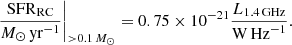 (1)
(1)
Hence, the radio continuum SFR surface density is (Heesen et al. 2014; Heesen & Buie 2019):
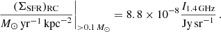 (2)
(2)
In our data, the intensity is measured in Jy beam−1. To convert from Jy sr−1 we use the full width at half maximum (FWHM) of the synthesised beam measured in arcsec. The solid angle subtended by a Gaussian beam relates to its area as Ω = 2.66 × 10⁻¹¹ × FWHM2 sr. We will also be using Condon’s relation at different radio frequencies. Thus, we scale with the frequency, ν, relative to 1.4 GHz, assuming a simple power law Iν ∝ να with a radio spectral index of α = −0.8. Of course, this is a simplification since the radio continuum spectrum cannot be described with a single power-law, but there is spectral curvature (Chyży et al. 2018). Also this spectral index applies to galaxies at gigahertz frequencies for the total radio continuum emission (including both the thermal and non-thermal emission; Tabatabaei et al. 2017) whereas the spectrum is flatter at lower frequencies (Marvil et al. 2015). We note that the choice of the radio spectral index does not influence our results since the calibration is relative: Eq. (1) is our definition and we then calibrate any deviations from it.
Our final modified version of Condon’s relation is now expressed as:
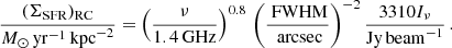 (3)
(3)
We also calculated radio spectral indices as
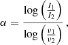 (4)
(4)
with the corresponding uncertainties (see Heesen et al. 2022, for details).
Our analysis was done using the software radio–pixel–plots (RPP)2. As input, it requires two radio maps and one hybrid ΣSFR map, prepared as described above and which calculates the spatially resolved (pixel by pixel) SFR surface densities from the radio maps using Condon’s relation. Then it maps the results pixel-by-pixel onto the SFR map, performs a double logarithmic linear fit and plots the result.
In order to calculate the map noise, σrms, a box-shaped region is defined in an area where no sources are visible. Furthermore, the pixels from the original image are averaged into new, larger ones with a size of 1.2 kpc. Let d be the distance to the galaxy in Mpc, h the side length of an original pixel in arcsecond, and r the desired resolution (the new pixel size) in pc, then the ratio of original-to-new pixels along one image side:
 (5)
(5)
Here, RPP does allow this ratio to have non integer values. If an original pixel is only partially inside a new pixel, it contributes to the new value proportionally to the surface area inside the new pixel. After the resolution is converted to 1.2 kpc, we apply a 3σ cutoff. The resulting error is
 (6)
(6)
where ϵ = 0.05 is the calibration uncertainty. This error underestimates the absolute error of the LOFAR data which is about 10% (Shimwell et al. 2019), but this smaller error, dominated by the uncertainties in the deconvolution, is a good estimate because we are most interested in the spatial variation across maps. Since we need all three values (two radio and one SFR), any pixel that is below the 3σ threshold will be removed from maps. Finally, the coarse radio map is converted into SFR surface densities using Condon’s relation (Eq. (3)) and then mapped onto the SFR map. SFR surface densities from the radio continuum and the hybrid data are expected to follow a linear relation in a double logarithmic plot:
![Mathematical equation: $$ \begin{aligned} \log _{10} \left[ (\Sigma _{\text{SFR}})_{\text{RC}} \right] = a \log _{10} \left[ (\Sigma _{\text{SFR}})_{\text{hyb}} \right] + b \,, \end{aligned} $$](/articles/aa/full_html/2024/02/aa47394-23/aa47394-23-eq9.gif) (7)
(7)
where (ΣSFR)hyb denotes the hybrid SFR surface density. This is fitted to our data using the orthogonal distance regression (ODR) package which is part of the SCIPY Python library. It implements a FORTRAN algorithm of the same name and uses a modified Levenberg–Marquardt algorithm. It has the advantage of being able to deal with both x and y errors.
2.3. Smoothing experiment
As in Heesen et al. (2023a) we performed a smoothing experiment using RPP in order to measure the CRE transport length. To this end we linearise the spatially resolved radio-SFR relation by convolving the hybrid SFR maps with a Gaussian kernel. The choice of kernel is motivated by our assumption that diffusion (and not streaming or advection) is the mechanism for CRE transport in galactic discs, unlike in galactic haloes (e.g. Stein et al. 2023). Otherwise, the kernel would be exponential instead. We define the CRE transport length lCRE as half of the FWHM of the Gaussian kernel. Following Heesen et al. (2014), we define the transport length equal to the diffusion length and the conversion from FWHM is:
 (8)
(8)
where σxy is the standard deviation of the Gaussian kernel. In order to estimate the uncertainty of lCRE, we assumed that the slope of the radio-SFR relation is 1.00 ± 0.05, where the uncertainty of the slope will then be translated into the uncertainty of lCRE (Heesen & Buie 2019). Further details of this method can be found in Heesen et al. (2023b).
The above experiment assumes isotropic diffusion employing a circular kernel. However, we also tested the possible influence of anisotropic diffusion. Several galaxies in our sample have inclination angles of i > 60°. If we assume anisotroic diffusion in the disc plane following the plane-parallel magnetic field, the projected diffusion length along the minor axis would have to be corrected with factors of cos(i) < 1/2. To test whether this would change our results we modified the convolution kernel to account for the geometric projection effect. The Gaussian2DKernel can be used as an elliptical kernel by providing a standard deviation for each coordinate direction: σx and σy. In terms of the previous standard deviation, σxy, we define them as
 (9)
(9)
The orientation of the ellipse can be changed through an additional angle, θ, which is the position angle of the major axis.
3. Results
3.1. Spatially resolved radio continuum-star formation rate relation
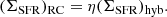
The spatially resolved analysis shows that the data points follow a sublinear radio-SFR relation for both frequencies 144 and 1365 MHz (Figs. 1a,b). The slope of the relation is flatter for lower frequencies which is expected because we see an older and therefore lower energy population of CREs, which had more time to diffuse. We divide the points into three groups based on their radio spectral indices: young CREs (−0.65 < α < −0.20; ≲30 Myr), medium age CREs (−0.85 < α < −0.65; 30–100 Myr) and old CREs (α < −0.85; ≳100 Myr). The values for the spectral indices are typical values found in the spiral arms, inter arm regions and outskirts of galaxies, respectively.
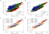 |
Fig. 1. Combined radio-SFR plots. Panels a and b show the radio ΣSFR at 144 and 1365 MHz, respectively, as function of the hybrid ΣSFR. Data points are colour-coded, so that young CREs are shown in red, middle-aged CREs are shown in green, and old CREs are shown in blue. Panels c and d show the relation only for young CREs, where the various galaxies are now colour-coded. Solid lines show in blue the 1:1 Condon’s relation and in orange the best-fitting power-law relations with 3σ confidence intervals indicated by dashed lines. Details of the best-fitting relations can found in Table 2. |
Focusing just on the young CREs (Figs. 1c,d), we see the slopes of their radio-SFR relations are a lot closer to unity and there is no significant difference between the frequencies. This behaviour is explained by the fact that the young CREs have energy spectra very close to their injection spectra. They have not propagated far from their sources and thus have not lost a lot of energy. This implies their spatial distribution should more closely resemble that of the star formation and they should therefore follow Condon’s relation more closely. The results are shown in Table 2.
Radio-SFR relation and CRE transport lengths in galaxies of the sample.
3.2. Influence of the calorimetric efficiency
In this section we investigate the influence of the calorimetric efficiency on the radio-SFR relation. The calorimetric efficiency is defined as the relative energy loss of the CREs due to synchrotron radiation (Pfrommer et al. 2022; Heesen et al. 2023b). Hence, we assume:
 (10)
(10)
In Figs. 2a,b we show a probability density distribution of log10[(ΣSFR)RC/(ΣSFR)hyb], the logarithmic ratio of radio-to-hybrid SFR surface density, separately for our three radio spectral index bins. While the distribution for young CREs is centred around −0.3–0, equating to ratios of 0.5–1, so that the radio and hybrid approximately ΣSFR agree, for middle-aged and old CREs the distribution is markedly different. For old CREs the distribution is centred around 0.7–0.9, equating to ratios of 5–8, which is greater than 1, so that the radio ΣSFR is significantly higher than the hybrid ΣSFR. This effect is even more pronounced for 144 MHz when compared with 1365 MHz.
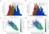 |
Fig. 2. Ratio of radio to hybrid ΣSFR. Top panels show histograms of the ratio separately for the three radio spectral index bins at 144 MHz (panel a) and 1365 MHz (panel b). Data points representing young CREs are in red, middle-aged CREs are in green, and old CREs are in blue, respectively. Best-fitting Gaussian distributions are shown as solid lines. Bottom panels show the ratio as function of the radio spectral index between 144 and 1365 MHz for 144 MHz (panel c) and 1365 MHz (panel d). Best-fitting exponential functions (Eq. (11)) shown as solid lines. |
In the next step we quantified this dependence further by studying the ratio of radio-to-hybrid ΣSFR as function of radio spectral index. This is shown in Figs. 2c,d. We find a clear correlation between the ratio and the radio spectral index. Such a behaviour can be explained by a varying calorimetric efficiency of the CRE, so that the calorimetric efficiency can be parametrised by the radio spectral index
![Mathematical equation: $$ \begin{aligned} \nonumber&\eta (\alpha )_{144\,\mathrm{MHz}} = \exp [(-5.85\pm 0.08) \alpha -(3.43\pm 0.06)]\\&\eta (\alpha )_{1365\,\mathrm{MHz}} = \exp [(-3.86\pm 0.08) \alpha -(1.82\pm 0.06)]. \end{aligned} $$](/articles/aa/full_html/2024/02/aa47394-23/aa47394-23-eq13.gif) (11)
(11)
Recall that if the CREs lose a large fraction of their energy, the radio spectral index becomes α = αinj − 0.5, where αinj is the injection spectral index. In contrast, if the CREs lose almost no energy via synchrotron radiation losses, then we expect a radio spectral index similar to the injection spectral index. Thus, we expect the calorimetric efficiency to be a function of radio spectral index as we have now confirmed.
We can now attempt to correct for the calorimetric efficiency by parametrising it by the radio spectral index and then divide the radio ΣSFR value by this (Eq. (10)). The corrected radio ΣSFR is then:
 (12)
(12)
In Fig. 3, we show the resulting radio-SFR relation. We can now see that this correction is able to restore a linear relation in close agreement with Condon’s relation. We also show the mean values binned in hybrid ΣSFR. The best-fitting relations are presented in Table 2.
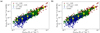 |
Fig. 3. Combined radio-SFR plots corrected for the CRE calorimetric efficiency at 144 (panel a) and 1365 MHz (panel b). We show the radio ΣSFR, which we have corrected with the parametrisation of the calorimetric efficiency as function of the radio spectral index, as function of the hybrid ΣSFR. The 1:1 Condon’s relation is shown as blue line. Data points are coloured according to the 144–1365 MHz radio spectral index. Yellow stars show mean values. The best-fitting power-law relations are not shown as they are virtually in agreement with Condon’s relation (see Table 2 for details). |
3.3. Cosmic-ray transport lengths
The principal results from the smoothing experiment are the CRE transport lengths (Table 2). At 144 MHz, we find a mean CRE transport length of ⟨l1⟩ = 3.5 ± 1.4 kpc and at 1365 MHz, we find ⟨l2⟩ = 2.4 ± 1.0 kpc. First, we would like to rule out that the size of our galaxies has any systematic effect when measuring the CRE transport lengths. In Fig. 4, we plot the transport lengths as a function of the star-formation radii. We find no significant correlation between lCRE and r⋆ with a Spearman rank correlation coefficient of ρs = 0.22. However, we find that the diffusion length is limited by the size of the galaxy with lCRE < r⋆/2. The diffusion length cannot be greater than the size of the galaxy. If the galaxies are too small, it may be impossible to detect older CREs effectively. Their lifetimes are so large and their transport lengths so long that they escape the galaxy before losing a lot of their energy. Outside the galaxy, the magnetic field strength is weak and therefore these electrons become undetectable. Secondly, it is hard to accurately measure values for lCRE that are smaller than the resolution of our maps; hence, ≈1 kpc is the lower limit we can detect with this method.
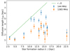 |
Fig. 4. Diffusion length as a function of galaxy star-forming radius. Blue data points correspond to 144 MHz and orange ones to 1365 MHz. The dashed line shows the relation lCRE = r⋆/2. |
Next, we investigated the possible influence of the inclination angle on the CRE transport length. We show the resulting diffusion lengths as a function of the geometric correction factor (see Eq. (9)) in Fig. 5. Again, we would expect no influence as the transport length of cosmic rays in the disc should be independent of inclination angle. For the isotropic diffusion kernel, this is indeed the case as the CRE transport length at 144 MHz is almost equal whether or not it is measured in galaxies at low (cos(i) > 0.5) or high (cos(i) < 0.5) inclination angles. On the other hand, for the anisotropic diffusion kernel, we find lCRE = 4.0 ± 0.4 kpc at low and lCRE = 7.7 ± 0.9 kpc at high inclination angles. Hence, we find that the anisotropic diffusion clearly overestimates the CRE transport length in the latter galaxies. This justifies our decision not to correct for the inclination angle because the cosmic rays diffuse in isotropic fashion, so there is no strong preferential diffusion in the disc plane of the galaxies (see also Murphy et al. 2008).
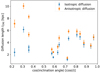 |
Fig. 5. Diffusion length as a function of the geometric correction due to the inclination angle cos(i). Blue data points show isotropic diffusion and orange data points show anisotropic diffusion at 144 MHz, respectively. |
3.4. Cosmic-ray electron transport
In this section, we investigate the properties of CRE transport in more detail. We calculate the electron lifetime for which we use estimates of the total magnetic field strength. We use the measurements of Heesen et al. (2023b) who used the revised equipartition formula by Beck & Krause (2005) and the 144 MHz maps together with the low-frequency radio spectral index. For the additional galaxies not included in the sample of Heesen et al. (2023b), we used values from the literature (see Table 1 for details). In order to take inverse Compton losses into account, we calculated the radiation energy density, Urad. Here, we follow the approach used in Heesen et al. (2018) by combining the CMB energy density, which can be measured directly, and the total radiation energy density, which is estimated using the total infrared luminosity.
Then we investigated diffusion lengths in relation to SFR surface densities (Fig. 6). Murphy et al. (2008) found that high SFR densities lead to lower CRE transport lengths. The reasoning is that more SFR density means more supernovae which lead to more shocks and amplify the B field in a galaxy. That should decrease the average transport length because synchrotron losses increase with magnetic field strength. We find only tentative indication of such a correlation (ρs = −0.42); however, if we leave out NGC 4254, which is affected by both the ram pressure and strong gravitational perturbation (Vollmer et al. 2005; Chyży et al. 2007; Duc & Bournaud 2008; Boselli et al. 2018), the correlation is improved, namely, to ρs = −0.57. We then explored the correlation with the equipartition magnetic field strength in Fig. 7 and found a weaker correlation with ρs = −0.45 (and ρs = −0.32 including NGC 4254). This could indicate that it is not only the magnetic field strength, but also the CRE lifetime that determine the transport length.
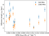 |
Fig. 6. Diffusion length as a function of the star formation rate surface density (SFRD). Data points are the same as in Fig. 4. The two data points on the right correspond to NGC 4254. |
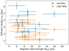 |
Fig. 7. Diffusion length as a function of the total magnetic field strength as estimated from energy equipartition. Data points as in Fig. 4. The two data points on the right correspond to NGC 4254. |
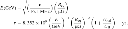
We can express the energy, E, and lifetime, τ, of the CREs as (Heesen & Buie 2019):
 (13)
(13)
where UB is the magnetic energy density. We can use the relation between CRE lifetime and transport length to discriminate between the different possible models of CRE transport. The models predict different scaling of CRE transport length, lCRE, and lifetime, τ, with frequency, ν. For diffusion, we expect ldiff ∝ ν−1/4, and for advection, ladv ∝ ν−1/2 (Vollmer et al. 2020). Another possibility we consider is an energy-dependent diffusion coefficient D(E)∝E1/2, which would cause a scaling proportional to ν−1/8. In general, for a diffusion coefficient D ∝ Eμ we expect ldiff ∝ ν(μ − 1)/4 (e.g. Heesen 2021). Since we can write τ ∝ ν−0.5, the diffusion length as a function of lifetime in a double logarithmic plot should follow a linear relation with the slope twice as high as when plotted versus frequency (Fig. 8). The data points show a relatively large scatter, although the correlation found here is the most significant yet (ρs = 0.61) when NGC 4254 is omitted. While our data are in agreement with energy-independent diffusion (μ = 0), we cannot rule out a modest energy dependence of the diffusion coefficient such as μ = 1/3; similarly, we cannot rule out cosmic-ray streaming either, even though the slope appears to be steeper than what has been observed.
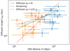 |
Fig. 8. Diffusion length as a function of CRE lifetime. Data points as in Fig. 4. Cosmic-ray transport models are shown for comparison. The green solid line shows energy-independent diffusion (μ = 0), the dashed red line shows streaming, and the purple dashed line shows the energy-dependent diffusion (μ = 1/3). The diffusion coefficient is parametrised as D ∝ Eμ. |
Another way to look at different cosmic-ray transport models is to directly compare the diffusion lengths at two different frequencies. We compute l1/l2 for our sample, which is the ratio of 144 to 1365 MHz CRE transport lengths. The results are shown in Table 2. The mean value is ⟨l1/l2⟩ = 1.44 ± 0.24. This value lies between the theoretical value for energy-dependent diffusion of 1.32 and energy-independent diffusion of 1.75. However, there are reasons why energy-independent diffusion is more likely. If we ignore CRE escape completely, our results would suggest some galaxies have energy-dependent diffusion, while others have energy-independent diffusion. In that case, we would have to find an explanation why different galaxies have different transport mechanisms. It is more likely that the galaxies with low ratios have faster CRE escape than those with high ratios. There are only two galaxies that have ratios in excess of what is expected for energy-dependent diffusion. This could be explained by cosmic-ray streaming or advection. These are NGC 4254 and 5055. In NGC 4254 this is expected as it has a radio tail where cosmic rays are advected or stream down the pressure gradient (Chyży et al. 2007). NGC 5055 is currently undergoing a minor merger with a disturbed outer disc (Chonis et al. 2011). Large-scale gas motions would lead to CRE advection explaining our results. We therefore conclude that our results make energy-independent CRE diffusion the most likely explanation.
3.5. Cosmic-ray diffusion and magnetic fields
Now that we have established that cosmic-ray diffusion can describe our data best, we investigate the influence of magnetic fields on CRE diffusion. To calculate the diffusion coefficient, D, we use the relation between lifetime, τ, and diffusion length, lCRE, for isotropic 3D diffusion as:
 (14)
(14)
The mean diffusion coefficient is ⟨D⟩=(1.07 ± 0.16)×1028 cm2 s−1.
In Fig. 9, we plot the diffusion coefficient as a function of the total magnetic field strength. There is a high variance in the values for the diffusion coefficients with no clear trend visible. The highest values are found in NGC 4254, where the radio tail will raise the values. The theory of 1D CRE diffusion in a disc suggests that the diffusion coefficient scales as follows (Shalchi et al. 2009):
 (15)
(15)
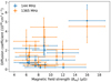 |
Fig. 9. Isotropic diffusion coefficient as function of total magnetic field strength, as estimated from energy equipartition in microgauss. Blue data points correspond to 144 MHz and orange ones to 1365 MHz. The data points on the right correspond to NGC 4254. |
where Bord is the ordered and Bturb is the turbulent magnetic field component, respectively. That means we should not expect to see a direct correlation with the total magnetic field strength Beq or perpendicular magnetic field strength B⊥. We cannot rule out any possible weak dependence of D on Beq. The high variance in the data and the small range of values for Beq would make it hard to detect.
The implied strong correlation of D with (Bord/Bturb)2 can be tested: the total perpendicular magnetic strength can be decomposed  . In principle, it is possible to measure two of those three: Beq is proportional to the total radio intensity and Bord is proportional to the polarised radio intensity (e.g. Tabatabaei et al. 2016). When linearly polarised radio waves traverse a plasma, they undergo a Faraday depolarisation. This process occurs both in the ISM and the Earth’s atmosphere and is proportional to ν−2. In practice, at low frequencies the radio continuum radiation is almost completely depolarised, making it very hard to directly probe the components of the magnetic field (see Table 1).
4. Discussion
4.1. Radio continuum-star formation rate relation
4.1.1. Semicalorimetric radio-SFR relation
In this work we calculated the spatially resolved radio-SFR relation in 15 nearby galaxies at a resolution of approximately (1.2 kpc)2. We used two different observing frequencies and found that for all of them, the slopes of the radio-SFR relation results for the full sample were smaller than 1. Specifically, we found a1 = 0.86 ± 0.02 at 144 MHz and a2 = 0.92 ± 0.01 at 1365 MHz. These results are in agreement with CRE transport that predict CREs move away from their places of origin. As a result, spots with high SFR surface densities will appear radio dim and places with low SFR surface densities will appear radio bright. That also explains the fact that the slope becomes flatter at lower frequencies. At lower frequencies we observe older CREs with a more smoothed out distribution. If we focus just on the young CREs (areas with spectral indices α > −0.65), the radio-SFR relation becomes almost linear with no apparent correlation with the frequency. We find a1 = 1.06 ± 0.02 at 144 MHz and a2 = 1.03 ± 0.02 at 1365 MHz. Those relations are expected to be steeper than the ones for all CREs, since young CREs have not had time to move very far from their origins. Hence, their distribution should be (almost) identical to the distribution of star formation. The fact that they follow a nearly linear relation could be a hint that there is some kind of local calorimetry at work. The CREs are somehow confined in the spiral arms and lose all their energy there.
In contrast, the global radio-SFR relation holds over five orders of magnitude and is super-linear, with most slopes reported between 1.1 and 1.4, where lower frequencies tend to have higher slopes (Li et al. 2016). The super-linear slope cannot be explained with a pure calorimeter model, which is why Niklas & Beck (1997) proposed an equipartition model. First, it requires the energy stored in cosmic rays and the magnetic field to be equal. Second, it proposes a feedback mechanism to explain the superlinearity: higher SFR leads to more gas turbulence which, in turn, amplifies the magnetic field. The increased magnetic field strength is then responsible for the increased synchrotron radiation. Their proposed relation is (see also Schleicher & Beck 2013):
 (16)
(16)
where α ≈ −0.6 is the CRE radio spectral index at injection.
There are however some recent results that seem to point more towards a semi-calorimetric model, where the escape of CREs play also a role. A large study by Smith et al. (2021) found an (almost) linear radio-SFR relation at low radio frequencies (1.041 ± 0.007) in line with earlier results from Gürkan et al. (2018), who used a similar methodology with a smaller sample. Gürkan et al. (2018) and Smith et al. (2021) also both found a mass dependence of their radio-SFR relation. At a constant SFR, the more massive a galaxy is, the more luminous it is in the radio continuum. It would be difficult to explain this behaviour with a calorimetric model alone. That is why the authors suggest that mass dependent CRE escape in these galaxies could be the reason for their findings. Chyży et al. (2018) investigated integrated radio spectral indices in star-forming galaxies and found that they were flatter than their injection indices α ≈ −0.57. When the sample was restricted to frequencies above 1.5 GHz, the radio spectra became steeper with α ≈ −0.77. If galaxies were perfect calorimeters we should see an integrated radio spectral index of α ≈ −1.1. Since that is not the case, there seems to be significant escape of CREs, particularly below 1 GHz.
4.1.2. Updated radio-SFR calibration
Hence, we now probe the effect of applying the calorimetric correction (Sect. 3.2) on the integrated radio-SFR relation. We can write the integrated radio-SFR relation as
 (17)
(17)
where we have used the calorimetric efficiency parametrised by the radio spectral index as given by Eq. (11). We used the 45 galaxies of Heesen et al. (2022) with the result shown in Fig. 10. The best-fitting relation has a slope of c = 1.02 ± 0.07 with LC = 1021.67 ± 0.04 W Hz−1. Notably, the relation is now almost linear and in excellent agreement with the slope of the spatially resolved relation. The constant LC is in excellent agreement with what is predicted by the spatially resolved relation (Eq. (3)). Combined with our two measurements and using the spatially resolved observations, our best estimate for the slope of the radio-SFR relation is 1.01 ± 0.02.
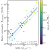 |
Fig. 10. Integrated radio-SFR relation but corrected for calorimetric efficiency parametrised by the radio spectral index. Blue line and shades areas show best-fitting relation with uncertainties. Dashed lines show 1σ scatter of data points. |
This means that we have for the first time identified a universal radio-SFR relation that can both be applied to integrated as well as spatially resolved measurements. This means that the observed variation in the slope of the radio-SFR relation can be explained by the influence of the CRE calorimetric efficiency. This was already proposed by Smith et al. (2021), who speculated that a higher mass leads to higher efficiency. This was corroborated by Heesen et al. (2022) who found a correlation between radio spectral index and total mass. A similar relation was found for galaxies in the Virgo cluster in the LOFAR survey by Edler et al. (2023a,b). The finding that this can also explain the local radio-SFR relation strongly corroborates this interpretation. We can now provide updated calibrations of the radio-SFR relation that absorbs the calorimetric efficiency into the radio continuum luminosity. To this end, we combined the radio spectral index–SFR relation (Heesen et al. 2022) with Eq. (11) to obtain:
 (18)
(18)
With this we can expand Condon’s relation to correct for the CRE calorimetric efficiency
 (19)
(19)
to obtain our new calibration
 (20)
(20)
where LN1 = 6.80 × 10²¹ W Hz−1 and LN2 = 1.84 × 10²¹ W Hz−1 is the radio continuum luminosity of a galaxy with SFR = 1 M⊙ yr−1 at 144 and 1365 MHz, respectively. This calibration is valid for 0.1 ≲ SFR/(M⊙ yr−1)≲10 and for total masses within the star-forming disc of 109 ≲ Mtot/M⊙ ≲ 1011. Our calibration at 1365 MHz is in reasonable agreement with the prescription by Bell (2003), who also took the non-linearity of the radio-SFR relation into account.
One other point is that the slope of the relation can also change with respect to the SFR tracer that is used (Bell 2003; Boselli et al. 2015). This effect can be related to the large uncertainty in the data and to the age dependencies on the SFR tracers, as well as to the determination of SFR from the observed data once corrected for dust attenuation. A question hopefully to be answered in the future is whether our simple model is still valid when a different star formation tracer is used. Another question is the influence of the underlying assumption of the radio-SFR relation that the SFR has been constant over a few CRE radiative life-times. Otherwise, relatively fast variations in SFR would induce an excess or deficiency in the radio luminosity-SFR relation, as tentatively shown Ignesti et al. (2022) for extreme jellyfish galaxies.
4.2. Cosmic-ray electron transport
We show in this work that the most likely transport mechanism for CREs in our galaxy sample is energy-independent diffusion. This is in agreement with our previous results for CRE diffusion in the disc of NGC 5194, where we analysed five frequencies at 54–8350 MHz (Heesen et al. 2023a). In Dörner et al. (2023), we showed that 3D simulations of energy-independent diffusion with advection in a galactic wind can explain the radio continuum data of this galaxy. Also, in edge-on galaxies, we do find similar results where the diffusion coefficient is energy-independent in galaxies that do not have a galactic wind (Heesen et al. 2022; Stein et al. 2023).
In summary, we find that CRE transport is energy independent in the energy range of a few GeV (< 10 GeV). Theoretical explanations for energy-independent diffusion include field line random walk, where the cosmic rays simply follow the magnetic field lines that are randomised and bent by turbulence (Minnie et al. 2009); alternatively, cosmic rays are scattered in turbulence that they generate themselves in the so-called self-confinement picture (Zweibel 2013); lastly, cosmic rays may be scattered in extrinsic turbulence that is generated in the interstellar medium such as by supernovae and stellar winds. We refer to Heesen et al. (2023a) for more information and references.
Any theory has to be able to explain why there appear to be two types of galaxies, namely: those with diffusive haloes and those with advective haloes. Galaxies that have sufficiently high SFR surface densities can possess galactic winds that may be even cosmic ray-driven (Breitschwerdt et al. 1991; Everett et al. 2008). On the other hand, galaxies that are rather quiescent do not have galaxy-wide winds so that the cosmic-ray transport appears of diffusive fashion. The self-confinement picture would be able to do this (Zweibel 2013), but also more diffusive transport modes are able to drive galactic winds (Wiener et al. 2017).
While our results appear to be at first glance in contradiction to some Earth-based measurements, we need to keep in mind the different energy range. The observed change of primary-to-secondary cosmic rays that suggest an energy-dependent diffusion coefficient (Becker Tjus & Merten 2020), apply to energies of > 10 GeV. In contrast, our data probe lower energy CREs with energies of less than 10 GeV, whereas the solar wind prevents this kind of measurement near the Earth. In this energy range there appears to be a flattening of the cosmic-ray spectrum as suggested by PAMELA and more importantly by Voyager data, which could point to a similar change in the transport mode (Blasi et al. 2012).
5. Conclusions
Radio continuum emission can be used as an extinction-free star formation tracer. This is motivated by the existence of a radio-SFR relation both globally between galaxies and spatially resolved within galaxies. The link between radio continuum emissions and star formation are CREs and their interactions with the ambient magnetic field. We want to understand the mechanism of CRE transport and spectral ageing using their radio spectral indices in order to calibrate the local radio-SFR relation. Such a calibration would allow us to measure SFRs in galaxies at higher redshifts with future surveys such as the Square Kilometre Array (SKA). We investigated a sample of 15 nearby face-on galaxies with data from WSRT, MeerKAT, SINGS, and LOFAR at two different radio frequencies of 144 and 1365 MHz. Low-frequency data are almost uncontaminated by thermal (free-free) emission. We followed the approach by Heesen et al. (2014), where the radio-SFR relation is measured at a spatial resolution of (1.2 kpc)2 and the radio continuum emission is compared with SFR surface densities using a hybrid prescription of far-ultraviolet and mid-infrared data (Leroy et al. 2008, 2012).
In agreement with earlier studies (e.g. Berkhuijsen et al. 2013; Vollmer et al. 2020), we find the SFR maps are smeared-out versions of the radio maps due to CRE transport resulting in sublinear radio-SFR relations. We linearise the radio-SFR relation by convolving the SFR maps with a Gaussian kernel, where the kernel size defines the CRE transport length. We find that the spatially resolved radio-SFR relations have sublinear slopes that move closer to linearity with increasing frequency (Figs. 1a,b). The trend has also been found in other studies (e.g. Heesen & Buie 2019) and supports the idea of CRE transport and spectral ageing. This is corroborated by the radio-SFR relation being nearly linear if we restrict our study to areas with young CRE (Figs. 1c,d). We now investigated the deviation of the local radio-SFR relation as a function of radio spectral index (Fig. 2). The ratio of radio-to-hybrid SFR surface density is then defined as the CRE calorimetric efficiency (Eq. (11)), which can be parametrised by the radio spectral index (Eq. (10)). After correcting the radio-SFR relation for the calorimetric efficiency, our main result is shown in Fig. 3. The corrected radio-SFR relation is now almost in agreement with a linear relation.
The smoothing experiment shows that lower energy CREs traced by lower frequencies have longer transport lengths that cannot exceed about half of the radius of the star-forming disc (Fig. 4). The CRE diffusion length has weakly significant correlation with SFR surface density, as shown in Fig. 6. This was already found by Murphy et al. (2008) and is interpreted by higher magnetic field strengths in areas of higher SFR (Heesen et al. 2023b; Pfrommer et al. 2022). This is corroborated by a weak correlation between CRE transport length and lifetime (Fig. 8). However, there is no significant correlation between CRE diffusion length and total magnetic field strength (Fig. 7), so that the CRE is not the only influence that determines the transport length. The magnetic field structure is likely of importance too. The relation between CRE transport length and lifetime shown in Fig. 8 is in best agreement with energy-independent diffusion. This is also the case when we consider the ratio of CRE transport length at 144 to that at 1365 MHz (Table 2). This is in agreement with earlier studies (Heesen et al. 2023a; Dörner et al. 2023) and applies to low-energy GeV CREs. We note that our observations of CRE transport apply only to a globalised measurement on kpc-scales, where there will be some confusion with the halo emission (Stein et al. 2023).
Arguably, the most exciting aspect of our study is the application of the corrected radio-SFR relation to integrated measurements. If we parametrise the calorimetric efficiency by the radio spectral index and apply this as a correcting factor to the integrated radio-SFR relation of the same LoTSS-DR2 galaxies (Heesen et al. 2022), we find the same linear radio-SFR relation as for the spatially resolved measurement (Fig. 10). As the normalisation of the integrated radio-SFR relation (Eq. (17)) agrees with the spatially resolved one (Eq. (1)), we have thus identified a potentially universal radio-SFR relation that applies to both global and local measurements. In particular, we are now also able to correct global measurements for the CRE calorimetric efficiency with the help of the radio spectral index. This means that in the future, we may be able to reduce the systematic uncertainties of the radio-SFR relation that have limited the applicability of deep radio continuum surveys in measuring cosmic SFRs. This will be possible thanks to future surveys with LOFAR, MeerKAT, and the SKA.
Assuming the cosmic-ray number density is N(E)∝E−γ, where E is the energy. The (non-thermal) radio spectral index is then α = (1 − γ)/2 where the radio continuum intensity scales with the frequency as Iν ∝ να.
https://github.com/sebastian-schulz/radio-pixel-plots
Acknowledgments
We thank the anonymous referee for a constructive report that helped to improve the clarity of the paper. LOFAR (van Haarlem et al. 2013) is the Low Frequency Array designed and constructed by ASTRON. It has observing, data processing, and data storage facilities in several countries, that are owned by various parties (each with their own funding sources), and that are collectively operated by the ILT foundation under a joint scientific policy. The ILT resources have benefitted from the following recent major funding sources: CNRS-INSU, Observatoire de Paris and Université d’Orléans, France; BMBF, MIWF-NRW, MPG, Germany; Science Foundation Ireland (SFI), Department of Business, Enterprise and Innovation (DBEI), Ireland; NWO, The Netherlands; The Science and Technology Facilities Council, UK; Ministry of Science and Higher Education, Poland. M.B. acknowledges funding by the Deutsche Forschungsgemeinschaft (DFG, German Research Foundation) under Germany’s Excellence Strategy – EXC 2121 ‘Quantum Universe’ – 390833306. M.S. acknowledges funding from the German Science Foundation DFG, within the Collaborative Research Center SFB1491. This research has made use of the NASA/IPAC Extragalactic Database (NED), which is operated by the Jet Propulsion Laboratory, California Institute of Technology, under contract with the National Aeronautics and Space Administration. This work made use of the SCIPY project https://scipy.org.
References
- Abramowski, A., Acero, F., Aharonian, F., et al. 2012, ApJ, 757, 158 [NASA ADS] [CrossRef] [Google Scholar]
- Ackermann, M., Ajello, M., Allafort, A., et al. 2012, ApJ, 755, 164 [NASA ADS] [CrossRef] [Google Scholar]
- Adriani, O., Akaike, Y., Asano, K., et al. 2018, Phys. Rev. Lett., 120, 261102 [NASA ADS] [CrossRef] [Google Scholar]
- Aharonian, F., Akhperjanian, A. G., Bazer-Bachi, A. R., et al. 2007, A&A, 464, 235 [NASA ADS] [CrossRef] [EDP Sciences] [Google Scholar]
- Basu, A., Roy, S., & Mitra, D. 2012, ApJ, 756, 141 [NASA ADS] [CrossRef] [Google Scholar]
- Beck, R., & Krause, M. 2005, Astron. Nachr., 326, 414 [Google Scholar]
- Becker Tjus, J., & Merten, L. 2020, Phys. Rep., 872, 1 [NASA ADS] [CrossRef] [Google Scholar]
- Bell, E. F. 2003, ApJ, 586, 794 [Google Scholar]
- Berkhuijsen, E. M., Beck, R., & Tabatabaei, F. S. 2013, MNRAS, 435, 1598 [Google Scholar]
- Beswick, R., Brinks, E., Perez-Torres, M., et al. 2015, in Advancing Astrophysics with the Square Kilometre Array (AASKA14), 70 [Google Scholar]
- Blasi, P., Amato, E., & Serpico, P. D. 2012, Phys. Rev. Lett., 109, 061101 [Google Scholar]
- Boselli, A., Fossati, M., Gavazzi, G., et al. 2015, A&A, 579, A102 [NASA ADS] [CrossRef] [EDP Sciences] [Google Scholar]
- Boselli, A., Fossati, M., Cuillandre, J. C., et al. 2018, A&A, 615, A114 [NASA ADS] [CrossRef] [EDP Sciences] [Google Scholar]
- Braun, R., Oosterloo, T. A., Morganti, R., Klein, U., & Beck, R. 2007, A&A, 461, 455 [NASA ADS] [CrossRef] [EDP Sciences] [Google Scholar]
- Breitschwerdt, D., McKenzie, J. F., & Völk, H. J. 1991, A&A, 245, 79 [NASA ADS] [Google Scholar]
- Calzetti, D., Kennicutt, R. C., Engelbracht, C. W., et al. 2007, ApJ, 666, 870 [Google Scholar]
- Chonis, T. S., Martínez-Delgado, D., Gabany, R. J., et al. 2011, AJ, 142, 166 [NASA ADS] [CrossRef] [Google Scholar]
- Chyży, K. T., Ehle, M., & Beck, R. 2007, A&A, 474, 415 [NASA ADS] [CrossRef] [EDP Sciences] [Google Scholar]
- Chyży, K. T., Jurusik, W., Piotrowska, J., et al. 2018, A&A, 619, A36 [NASA ADS] [CrossRef] [EDP Sciences] [Google Scholar]
- Condon, J. J. 1992, ARA&A, 30, 575 [Google Scholar]
- Davies, L. J. M., Huynh, M. T., Hopkins, A. M., et al. 2017, MNRAS, 466, 2312 [Google Scholar]
- Dörner, J., Reichherzer, P., Becker Tjus, J., & Heesen, V. 2023, A&A, 669, A111 [NASA ADS] [CrossRef] [EDP Sciences] [Google Scholar]
- Drury, L. O. 1983, Rep. Prog. Phys., 46, 973 [Google Scholar]
- Duc, P.-A., & Bournaud, F. 2008, ApJ, 673, 787 [NASA ADS] [CrossRef] [Google Scholar]
- Dumas, G., Schinnerer, E., Tabatabaei, F. S., et al. 2011, AJ, 141, 41 [NASA ADS] [CrossRef] [Google Scholar]
- Edler, H. W., de Gasperin, F., Shimwell, T. W., et al. 2023a, A&A, 676, A24 [NASA ADS] [CrossRef] [EDP Sciences] [Google Scholar]
- Edler, H. W., Roberts, I. D., Boselli, A., et al. 2023b, A&A, submitted [arXiv:2311.01904] [Google Scholar]
- Everett, J. E., Zweibel, E. G., Benjamin, R. A., et al. 2008, ApJ, 674, 258 [CrossRef] [Google Scholar]
- Gaisser, T. K., Stanev, T., & Tilav, S. 2013, Front. Phys., 8, 748 [NASA ADS] [CrossRef] [Google Scholar]
- Gürkan, G., Hardcastle, M. J., Smith, D. J. B., et al. 2018, MNRAS, 475, 3010 [Google Scholar]
- Heald, G., Braun, R., & Edmonds, R. 2009, A&A, 503, 409 [NASA ADS] [CrossRef] [EDP Sciences] [Google Scholar]
- Heesen, V. 2021, Ap&SS, 366, 117 [NASA ADS] [CrossRef] [Google Scholar]
- Heesen, V., Brinks, E., Leroy, A. K., et al. 2014, AJ, 147, 103 [NASA ADS] [CrossRef] [Google Scholar]
- Heesen, V., Croston, J. H., Morganti, R., et al. 2018, MNRAS, 474, 5049 [Google Scholar]
- Heesen, V., Buie, E. I., Huff, C. J., et al. 2019, A&A, 622, A8 [NASA ADS] [CrossRef] [EDP Sciences] [Google Scholar]
- Heesen, V., Staffehl, M., Basu, A., et al. 2022, A&A, 664, A83 [NASA ADS] [CrossRef] [EDP Sciences] [Google Scholar]
- Heesen, V., de Gasperin, F., Schulz, S., et al. 2023a, A&A, 672, A21 [NASA ADS] [CrossRef] [EDP Sciences] [Google Scholar]
- Heesen, V., Klocke, T. L., Brüggen, M., et al. 2023b, A&A, 669, A8 [NASA ADS] [CrossRef] [EDP Sciences] [Google Scholar]
- Hindson, L., Kitchener, G., Brinks, E., et al. 2018, ApJS, 234, 29 [NASA ADS] [CrossRef] [Google Scholar]
- Ignesti, A., Vulcani, B., Poggianti, B. M., et al. 2022, ApJ, 937, 58 [NASA ADS] [CrossRef] [Google Scholar]
- Kapińska, A. D., Staveley-Smith, L., Crocker, R., et al. 2017, ApJ, 838, 68 [CrossRef] [Google Scholar]
- Kennicutt, R. C., Jr, Armus, L., Bendo, G., et al. 2003, PASP, 115, 928 [NASA ADS] [CrossRef] [Google Scholar]
- Leroy, A. K., Walter, F., Brinks, E., et al. 2008, AJ, 136, 2782 [Google Scholar]
- Leroy, A. K., Bigiel, F., de Blok, W. J. G., et al. 2012, AJ, 144, 3 [Google Scholar]
- Li, J.-T., Beck, R., Dettmar, R.-J., et al. 2016, MNRAS, 456, 1723 [NASA ADS] [CrossRef] [Google Scholar]
- Marvil, J., Owen, F., & Eilek, J. 2015, AJ, 149, 32 [CrossRef] [Google Scholar]
- Mertsch, P. 2018, J. Cosmol. Astropart. Phys., 2018, 045 [CrossRef] [Google Scholar]
- Minnie, J., Matthaeus, W. H., Bieber, J. W., Ruffolo, D., & Burger, R. A. 2009, J. Geophys. Res. (Space Phys.), 114, A01102 [Google Scholar]
- Mulcahy, D. D., Beck, R., & Heald, G. H. 2017, A&A, 600, A6 [NASA ADS] [CrossRef] [EDP Sciences] [Google Scholar]
- Murphy, E. J. 2009, ApJ, 706, 482 [Google Scholar]
- Murphy, E. J., Helou, G., Kenney, J. D. P., Armus, L., & Braun, R. 2008, ApJ, 678, 828 [Google Scholar]
- Murphy, E. J., Condon, J. J., Schinnerer, E., et al. 2011, ApJ, 737, 67 [Google Scholar]
- Murphy, E. J., Porter, T. A., Moskalenko, I. V., Helou, G., & Strong, A. W. 2012, ApJ, 750, 126 [NASA ADS] [CrossRef] [Google Scholar]
- Niklas, S., & Beck, R. 1997, A&A, 320, 54 [NASA ADS] [Google Scholar]
- Pakmor, R., van de Voort, F., Bieri, R., et al. 2020, MNRAS, 498, 3125 [NASA ADS] [CrossRef] [Google Scholar]
- Pfrommer, C., Werhahn, M., Pakmor, R., Girichidis, P., & Simpson, C. M. 2022, MNRAS, 515, 4229 [NASA ADS] [CrossRef] [Google Scholar]
- Ranasinghe, S., & Leahy, D. 2023, ApJS, 265, 53 [NASA ADS] [CrossRef] [Google Scholar]
- Schleicher, D. R. G., & Beck, R. 2013, A&A, 556, A142 [NASA ADS] [CrossRef] [EDP Sciences] [Google Scholar]
- Shalchi, A., Škoda, T., Tautz, R. C., & Schlickeiser, R. 2009, Phys. Rev. D, 80, 023012 [NASA ADS] [CrossRef] [Google Scholar]
- Shimwell, T. W., Röttgering, H. J. A., Best, P. N., et al. 2017, A&A, 598, A104 [NASA ADS] [CrossRef] [EDP Sciences] [Google Scholar]
- Shimwell, T. W., Tasse, C., Hardcastle, M. J., et al. 2019, A&A, 622, A1 [NASA ADS] [CrossRef] [EDP Sciences] [Google Scholar]
- Shimwell, T. W., Hardcastle, M. J., Tasse, C., et al. 2022, A&A, 659, A1 [NASA ADS] [CrossRef] [EDP Sciences] [Google Scholar]
- Smith, D. J. B., Haskell, P., Gürkan, G., et al. 2021, A&A, 648, A6 [EDP Sciences] [Google Scholar]
- Stein, M., Heesen, V., Dettmar, R. J., et al. 2023, A&A, 670, A158 [NASA ADS] [CrossRef] [EDP Sciences] [Google Scholar]
- Tabatabaei, F. S., Martinsson, T. P. K., Knapen, J. H., et al. 2016, ApJ, 818, L10 [NASA ADS] [CrossRef] [Google Scholar]
- Tabatabaei, F. S., Schinnerer, E., Krause, M., et al. 2017, ApJ, 836, 185 [Google Scholar]
- van de Voort, F., Bieri, R., Pakmor, R., et al. 2021, MNRAS, 501, 4888 [NASA ADS] [CrossRef] [Google Scholar]
- van Haarlem, M. P., Wise, M. W., Gunst, A. W., et al. 2013, A&A, 556, A2 [NASA ADS] [CrossRef] [EDP Sciences] [Google Scholar]
- Vollmer, B., Huchtmeier, W., & van Driel, W. 2005, A&A, 439, 921 [NASA ADS] [CrossRef] [EDP Sciences] [Google Scholar]
- Vollmer, B., Soida, M., Beck, R., & Powalka, M. 2020, A&A, 633, A144 [NASA ADS] [CrossRef] [EDP Sciences] [Google Scholar]
- Wiener, J., Pfrommer, C., & Oh, S. P. 2017, MNRAS, 467, 906 [NASA ADS] [Google Scholar]
- Zweibel, E. G. 2013, Phys. Plasmas, 20, 055501 [NASA ADS] [CrossRef] [Google Scholar]
All Tables
All Figures
|
Fig. 1. Combined radio-SFR plots. Panels a and b show the radio ΣSFR at 144 and 1365 MHz, respectively, as function of the hybrid ΣSFR. Data points are colour-coded, so that young CREs are shown in red, middle-aged CREs are shown in green, and old CREs are shown in blue. Panels c and d show the relation only for young CREs, where the various galaxies are now colour-coded. Solid lines show in blue the 1:1 Condon’s relation and in orange the best-fitting power-law relations with 3σ confidence intervals indicated by dashed lines. Details of the best-fitting relations can found in Table 2. |
| In the text | |
|
Fig. 2. Ratio of radio to hybrid ΣSFR. Top panels show histograms of the ratio separately for the three radio spectral index bins at 144 MHz (panel a) and 1365 MHz (panel b). Data points representing young CREs are in red, middle-aged CREs are in green, and old CREs are in blue, respectively. Best-fitting Gaussian distributions are shown as solid lines. Bottom panels show the ratio as function of the radio spectral index between 144 and 1365 MHz for 144 MHz (panel c) and 1365 MHz (panel d). Best-fitting exponential functions (Eq. (11)) shown as solid lines. |
| In the text | |
|
Fig. 3. Combined radio-SFR plots corrected for the CRE calorimetric efficiency at 144 (panel a) and 1365 MHz (panel b). We show the radio ΣSFR, which we have corrected with the parametrisation of the calorimetric efficiency as function of the radio spectral index, as function of the hybrid ΣSFR. The 1:1 Condon’s relation is shown as blue line. Data points are coloured according to the 144–1365 MHz radio spectral index. Yellow stars show mean values. The best-fitting power-law relations are not shown as they are virtually in agreement with Condon’s relation (see Table 2 for details). |
| In the text | |
|
Fig. 4. Diffusion length as a function of galaxy star-forming radius. Blue data points correspond to 144 MHz and orange ones to 1365 MHz. The dashed line shows the relation lCRE = r⋆/2. |
| In the text | |
|
Fig. 5. Diffusion length as a function of the geometric correction due to the inclination angle cos(i). Blue data points show isotropic diffusion and orange data points show anisotropic diffusion at 144 MHz, respectively. |
| In the text | |
|
Fig. 6. Diffusion length as a function of the star formation rate surface density (SFRD). Data points are the same as in Fig. 4. The two data points on the right correspond to NGC 4254. |
| In the text | |
|
Fig. 7. Diffusion length as a function of the total magnetic field strength as estimated from energy equipartition. Data points as in Fig. 4. The two data points on the right correspond to NGC 4254. |
| In the text | |
|
Fig. 8. Diffusion length as a function of CRE lifetime. Data points as in Fig. 4. Cosmic-ray transport models are shown for comparison. The green solid line shows energy-independent diffusion (μ = 0), the dashed red line shows streaming, and the purple dashed line shows the energy-dependent diffusion (μ = 1/3). The diffusion coefficient is parametrised as D ∝ Eμ. |
| In the text | |
|
Fig. 9. Isotropic diffusion coefficient as function of total magnetic field strength, as estimated from energy equipartition in microgauss. Blue data points correspond to 144 MHz and orange ones to 1365 MHz. The data points on the right correspond to NGC 4254. |
| In the text | |
|
Fig. 10. Integrated radio-SFR relation but corrected for calorimetric efficiency parametrised by the radio spectral index. Blue line and shades areas show best-fitting relation with uncertainties. Dashed lines show 1σ scatter of data points. |
| In the text | |
Current usage metrics show cumulative count of Article Views (full-text article views including HTML views, PDF and ePub downloads, according to the available data) and Abstracts Views on Vision4Press platform.
Data correspond to usage on the plateform after 2015. The current usage metrics is available 48-96 hours after online publication and is updated daily on week days.
Initial download of the metrics may take a while.