| Issue |
A&A
Volume 682, February 2024
|
|
|---|---|---|
| Article Number | A6 | |
| Number of page(s) | 14 | |
| Section | Planets and planetary systems | |
| DOI | https://doi.org/10.1051/0004-6361/202346820 | |
| Published online | 26 January 2024 | |
Optical constants of exoplanet haze analogs from 0.3 to 30 µm: Comparative sensitivity between spectrophotometry and ellipsometry★
1
University of Paris Saclay, OVSQ, LATMOS,
11 Boulevard d'Alembert,
78280
Guyancourt, France
e-mail: thomas.drant@latmos.ipsl.fr
2
Ludwig Maximilian University, Faculty of Physics, Observatory of Munich,
Scheinerstrasse 1,
Munich
81679, Germany
3
Ecole Polytechnique, LPICM, Route de Saclay,
91120
Palaiseau, France
4
NASA Ames Research Center, Space Science and Astrobiology Division,
Code ST,
Moffett Field, CA
94035, USA
5
LESIA, Observatoire de Paris, Université PSL, CNRS,
Sorbonne Université, 5 place Jules Janssen,
92195
Meudon, France
6
Synchrotron SOLEIL, L’Orme des Merisiers,
91190
Saint-Aubin, France
7
University of Bern, Center for Space and Habitability,
Gesellschaftsstrasse 6,
3012
Bern, Switzerland
8
University of Bern, ARTORG Center for Biomedical Engineering Research,
Murtenstrasse 50,
3008
Bern, Switzerland
9
University of Warwick, Department of Physics, Astronomy & Astrophysics Group,
Coventry
CV4 7AL, UK
Received:
5
May
2023
Accepted:
18
September
2023
We report new optical constants (refractive index, n, and extinction coefficient, k) for exoplanet haze analogs from 0.3 to 30 µm. The samples were produced in a simulated N2-dominated atmosphere with two different abundance ratios of CO2 and CH4, using the PAMPRE plasma reactor at LATMOS. We find that our haze analogs present a significantly lower extinction coefficient in the optical and near-infrared (NIR) range compared to the seminal data obtained on Titan haze analogs. We confirm the stronger IR absorption expected for hazes produced in a gas mixture with higher CO2 abundances. Given the strong impact of the atmospheric composition on the absorbing power of hazes, these new data should be used to characterize early-Earth and CO2-rich exoplanet atmospheres. The data presented in this paper can be found in the Optical Constants Database. Using ellipsometry or spectrophotometry, the retrieved optical constants are affected by the sensitivity of the measurement and the accuracy of the calculations. A comparative study of both techniques was performed to identify limitations and better understand the discrepancies present in the previous data. For the refractive index n, errors of 1–3% are observed with both optical techniques and the different models, caused by the correlation with the film thickness. We find that UV-visible reflection ellipsometry provides similar n values, regardless of the model used; whereas the Swanepoel method on transmission is more subjected to errors in the UV. In the UV and mid-infrared (MIR), the different calculations lead to rather small errors on k. Larger errors of k arise in the region of weak absorption, where calculations are more sensitive to errors on the refractive index n.
Key words: astrobiology / planets and satellites: atmospheres / planets and satellites: terrestrial planets
Data available in the Optical Constants Database: https://ocdb.smce.nasa.gov/
© The Authors 2024
 Open Access article, published by EDP Sciences, under the terms of the Creative Commons Attribution License (https://creativecommons.org/licenses/by/4.0), which permits unrestricted use, distribution, and reproduction in any medium, provided the original work is properly cited.
This article is published in open access under the Subscribe to Open model. Subscribe to A&A to support open access publication.
1 Introduction
Past observations and modeling predictions have taught us that aerosols are ubiquitous in exoplanet atmospheres (Gao et al. 2021). Their scattering-induced opacity mutes gaseous signatures challenging our effort to unveil the atmospheric composition (e.g., Wakeford & Sing 2015; Sing et al. 2016; Bruno et al. 2018). The process of aerosol formation is directly related to the physical-chemical properties of the atmosphere. Following future ambitions with the James Webb Space Telescope (JWST) and the Atmospheric Remote-sensing Infrared Exoplanet Large-survey (ARIEL), the characterization of aerosols represents an essential step in understanding the diversity and complexity of exoplanet atmospheres (Beichman et al. 2014; Heng & Showman 2015; Zellem et al. 2019; Lacy & Burrows 2020).
Photochemical hazes are direct evidence of a complex disequilibrium chemistry triggered by energetic photons in the upper atmosphere. They are expected in the H2-dominated atmospheres of relatively cold gas giants, where methane is the main form of carbon (Gao et al. 2020). Laboratory experiments also revealed that a broad variety of bulk compositions can lead to the formation of hazes, including CO2- and H2O-rich atmospheres (He et al. 2018a; Hörst et al. 2018). Given the broad diversity of atmospheric compositions predicted for rocky exoplanets (Gaillard & Scaillet 2014; Deng et al. 2020; Gaillard et al. 2022; Tian & Heng 2023), the presence of hazes is expected for numerous objects.
In atmospheric science, the gas-phase chemistry is described using a generalized framework based on first principles that can be used to predict the composition of exoplanet atmospheres (e.g., Heng et al. 2016). The complexity of haze formation precludes a similar description and requires the use of hefty assumptions for its physical parametrization (e.g., Morley et al. 2015; Lavvas & Koskinen 2017; Kawashima & Ikoma 2018, 2019; Gao et al. 2020). Laboratory analyses of the gas-phase chemistry and its complex effect on haze production clearly point to the presence of multiple chemical pathways depending on the initial gas mixture (Sciamma-O’Brien et al. 2017; He et al. 2018a,b; Hörst et al. 2018; Berry et al. 2019; Moran et al. 2020; Perrin et al. 2021). Our current knowledge of haze composition and optical properties therefore mainly relies on experimental data. Intrinsic properties of photochemical hazes are described with their refractive indices (n and k), also called optical constants, used as an input parameter for Mie theory (e.g., Kitzmann & Heng 2018). However, the data are scarce and often limited to a narrow spectral range (Gao et al. 2021).
The pioneering study of Khare et al. (1984) motivated the emergence of a field focusing on the formation of laboratory haze analogs, also called tholins, to retrieve their optical constants in support to observations and atmospheric modeling. Despite the different gas compositions expected for exoplanet atmospheres, the data of Khare et al. (1984) obtained on Titan haze analogs continue to be used for its broad spectral range (Arney et al. 2016; Kawashima & Ikoma 2018, 2019). A departure from a reduced N2/CH4 (Titan) composition towards more oxidizing conditions revealed the increased absorbing power of haze analogs (Gavilan et al. 2017, 2018; Jovanović et al. 2021), which can be partly explained by the incorporation of oxygen in the solid (Jovanović et al. 2020). A surprisingly high production rate of haze analogs with lower IR absorption properties is expected in H2O-rich atmospheres (He et al. 2018a; Hörst et al. 2018). Recent simulations suggest that these different absorbing properties would significantly impact IR transit spectra (He et al. 2023). In the era of JWST, haze particles could in theory be observed using their vibrational modes in the mid-infrared (MIR), along with the scattering slope in the visible and near-infrared (NIR) as well (Wakeford & Sing 2015; Pinhas & Madhusudhan 2017; Mai & Line 2019; He et al. 2023). Optical constants of exoplanet haze analogs are therefore needed in a broad spectral range for future analyses of JWST spectra.
Following the seminal work of Khare et al. (1984), more data were acquired on laboratory haze analogs, although they were often limited to either the MIR (Imanaka et al. 2012) or the UV–Vis–NIR (Ramirez et al. 2002; Mahjoub et al. 2012; Sciamma-O’Brien et al. 2012; Gavilan et al. 2017; Jovanović et al. 2021; He et al. 2022). The discrepancies in the reported optical constants are significant and largely overcome the uncertainties given by each study, even for haze analogs produced from a similar gas composition. The extinction coefficient (k) of Titan haze analogs measured by different groups varies by up to two orders of magnitude in the optical-NIR range (Brassé et al. 2015; He et al. 2022). Also, UV absorption is significantly different (Brassé et al. 2015), with only a few groups that observed a peak of absorption around 300–400 nm (Ramirez et al. 2002; He et al. 2022).
These discrepancies can be explained by three factors: the composition of the gas mixture, the experimental conditions (gas flow rate, pressure, temperature, energy distribution of the source, etc.) and the optical technique used to derive the refractive indices (Brassé et al. 2015). It was shown that relative abundances in the initial gas mixture affect the optical properties of hazes across the entire range (Mahjoub et al. 2012; Gautier et al. 2012; Gavilan et al. 2017, 2018). This assessment was possible as the analogs were produced using the same experimental setup and the measurements were performed using the same optical technique. The current data were, however, obtained by different groups, so the literature is thus split between optical constants measured with ellipsometry and spectrophotometry. To the best of our knowledge, comparison of ellipsometric and spectrophotometric calculations using a similar analog and spectral range were only reported by Tran et al. (2003). Their results, limited to the refractive index n in the optical range, suggest variations between both techniques. A study is long overdue to assess the effect of the optical method and better understand the current inconsistencies in the data.
The aim of the present study is two-fold. First, we assess the effect of the optical technique providing a new baseline study to guide future calculations of optical constants for exoplanet aerosol analogs. The sensitivities and limitations of the different methods are investigated to better understand the discrepancies in the existing data. Then, we provide new optical constants (n and k) for exoplanet haze analogs from 0.3 to 30 µm thus covering the entire spectral range of JWST and ARIEL. Our analogs are produced using different oxidations in the gas mixture to quantify the increased absorption expected for oxygenated hazes. Following the work of Gavilan et al. (2018), we provide additional refractive index calculations and expand the spectral coverage in the far-infrared (FIR). Our new data are compared to the seminal work of Khare et al. (1984) for Titan haze analogs in the context of our discussion of the implications for future observations.
2 Haze analogs
2.1 Production with PAMPRE
Haze analogs are produced using the PAMPRE (French acronym for “production of aerosols in micro-gravity by a reactive plasma”) experimental setup described in detail in Szopa et al. (2006). This plasma reactor triggers disequilibrium chemical reactions from electron impact at energies equivalent to vacuum-ultraviolet photons. The relative electron energy distribution is similar to a solar spectrum, with an increased high-frequency tail enhancing the dissociation and ionization of the gas molecules (Szopa et al. 2006; Alves et al. 2012). The plasma is confined in a stainless-steel cage with the base acting as the grounded electrode onto which we place optical substrates. During the experiment, an organic film grows on top of the substrates and pseudo-spherical grains are deposited on the reactor walls. To avoid an intricate treatment of the grain geometry, the refractive indices are only measured on thin films.
Experiments are performed at room temperature. The plasma is generated using a fixed radio-frequency power of 30 W and frequency of 13.56MHz. The gas mixture is injected in the PAMPRE reactor chamber from high-purity gas bottles (≥99.995% for CO2, ≥99.9999% for N2 and ≥99.9995% for CH4) using MKS mass flow rate controllers. A continuous injection at 60 sccm (standard cubic centimeter per minute) and primary pumping generate a gas flow and ensure a stable pressure of 0.85 hPa in the reactor chamber. The haze analogs are collected at the end of the experiment. The chamber is then pumped down to ~10−6 hPa using a turbo-molecular pump and the reactor walls are heated to prevent water contamination in the next experiments.
2.2 Gas mixture and samples
We mimic the composition of an oxidized Titan-like exoplanet atmosphere using the CO2-CH4 molecular pair recently proposed and currently debated as a potential biosignature (Arney et al. 2016, 2018; Krissansen-Totton et al. 2018; Woitke et al. 2021; Mikal-Evans 2022). The chosen gas composition is somewhat arbitrary given the wide diversity expected for exoplanet atmospheres (Gaillard & Scaillet 2014; Deng et al. 2020; Gaillard et al. 2022; Tian & Heng 2023), and is mainly inspired by our current knowledge on the chemical reactivity of N2 and CH4 (Sciamma-O’Brien et al. 2010). Our gas mixture is composed of 95% N2 with two different abundance ratios of CO2 and CH4. We focus on CHON haze analogs formed in N2-dominated gas mixtures to: (1) compare our optical constants obtained in a broad spectral range with the seminal data of Khare et al. (1984) and (2) assess the sensitivity of the different optical methods and calculations to understand discrepancies in the existing data and (3) quantify over a broad spectral range the change in optical properties emerging with higher abundances of CO2 (Gavilan et al. 2017, 2018).
The properties of the two haze analogs, including the composition of the gas mixtures, are detailed in Table 1. Henceforth, the analogs produced in a 1% and 3% CO2-rich gas mixture are referred to as the reduced and oxidized analog, respectively. For each gas mixture, thin films were deposited onto three different substrates during a single experiment. The substrates were specifically chosen to ensure the reliability of the subsequent ex situ spectroscopic and ellipsometric measurements. We used an MgF2 optical window (Crystran) for spectroscopic measurements in the UV-MIR range, an intrinsic silicon wafer (Sil’Tronix) with both sides polished for infrared spectroscopy, and a P-doped (boron) single side polished Si wafer (Sil’Tronix) for ellipsometric measurements. The different samples were produced with a thickness higher than 500 nm to avoid the formation of a non-negligible oxidized layer when they are exposed to air to carry out the optical measurements (Nuevo et al. 2022). The study of Gavilan et al. (2017) showed that an additional oxidized layer can be a limiting factor leading to model-dependent solutions when determining the refractive indices. Between the different optical measurements performed in this study, our samples were kept under primary vacuum to avoid continuous oxidation.
Different samples of our two haze analogs.
3 Optical measurements and calculations
3.1 Characterizing haze analogs with spectrophotometry and ellipsometry
3.1.1 Optical constants: Intrinsic optical properties
Even though the composition of hazes remains largely unknown, their intrinsic properties can be described by the refractive indices, also referred to as optical constants, that physically quantify dispersion and absorption of radiation independently of the particles’ geometry.
Dispersion and absorption result from dielectric polarization that occurs as electric dipoles within the material align with the electric field and oscillate following the frequency of the incident wave. In response to these forced oscillations, the dipoles radiate in all directions creating a secondary wave that interferes with the primary wave.
Sequential dielectric polarization reduces the speed of light in the material giving rise to the phenomenon of dispersion. The temporal frequency of light is unchanged in any medium but the wavelength is modified as λ/n, with λ being the vacuum wavelength and n the real part of the complex refractive index.
Resonant oscillations occur as the natural frequencies of the dipoles are approached, leading to destructive interference between the primary and secondary waves thus giving rise to the phenomenon of absorption. Electronic polarization occurs at optical and UV frequencies, whereas atomic polarization leads to absorption at infrared frequencies.
The complex refractive index is expressed as N = n + ik, where n is the refractive index and k is the extinction coefficient. Both are dimensionless parameters function of the composition, describing dispersion and absorption, respectively.
Absorption and dispersion occur at the same time, their causal relationship is expressed by the Kramers-Kronig equation (Kronig 1926; Kramers 1927):

where v is the vacuum wavenumber (cm−1, defined as 1/λ) and n∞ is the refractive index at infinite wavenumber, and P is the Cauchy principal value of the integral.
3.1.2 Spectrophotometry versus ellipsometry
Spectrophotometry and ellipsometry are the two main techniques used in material science to measure the refractive indices. Currently, the optical constants of haze analogs have been equally obtained with spectrophotometry (Khare et al. 1984; Ramirez et al. 2002; Tran et al. 2003; Imanaka et al. 2012; He et al. 2022) and ellipsometry (Khare et al. 1984; Mahjoub et al. 2012; Sciamma-O’Brien et al. 2012; Gavilan et al. 2017; Jovanović et al. 2021). The theory behind both techniques is very mature, we do not claim to bring any new theoretical contributions to the field but rather review the concepts that are relevant to understand the calculations discussed in the present study. Most of these concepts are adapted from the textbooks of Tompkins & Irene (2005) and Fujiwara (2007).
In practice, both methods rely on reflectance and/or transmittance measurements. Calculations account for the layered structure of the sample illustrated in Fig. 1. Reflection and transmission at the different interfaces between media is only function of the refractive indices (and incident angle), as described by the well-known Fresnel coefficients.
Spectrophotometry and ellipsometry however differ in the description of the intrinsic properties. In spectrophotometry, we use the complex refractive index to describe how a medium affects the propagation of the wave. This physical description is commonly used in astronomy and planetary science, taking its root in the fundamental wave equation. In practice, spectrophotometric measurements are usually performed under unpolarized light. In ellipsometry, intrinsic optical properties are defined by the dielectric constant, ε (ε = ε1 + iε2), also called dielectric function for ε(ν). Commonly used in material science, this formalism describes the behavior of oscillating electric dipoles in a solid structure. In practice, ellipsometry uses a grazing geometry and different polarization states of light to understand the behavior of the dipoles.
The difference between both methods therefore essentially emerges from the physical description, whether we focus on the wave or the material. Both definitions describe dispersion and absorption by the material using a different formalism. Calculations should in principle provide similar intrinsic properties to satisfy the known relation between ε and N:

In practice, the different models used for data analysis rely on specific assumptions that can lead to discrepancies in the retrieved optical constants. One aim of this study is to assess the limitations and sensitivities of the different methods applied to our haze analogs in a broad spectral range. In the next sections, we describe in detail the different measurements and calculations performed to retrieve the refractive indices from UV to FIR. For the comparative study of spectrophotometry and ellipsometry, we focus on the reduced analog (Table 1).
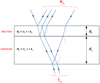 |
Fig. 1 Haze analog: Thin film (ƒ) overlaying a substrate (s). Each medium (or layer) is characterized by its thickness (d) and complex refractive index (N). df ≪ ds in practice, the scale is changed for clarity. The measured reflection and transmission of the film-substrate sample, Rfs and Tfs, respectively, are affected by multiple reflections at the different interfaces. |
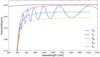 |
Fig. 2 Measured transmittance of the reduced analog deposited on a MgF2 substrate (Tfs, blue curve). The transmission of the substrate alone is shown with the black curve. The transmission envelopes (TM and Tm) and the interference-free transmission (Tα) are constructed based on the Swanepoel method. |
3.2 UV-Vis-NIR spectrophotometry
3.2.1 Measurements
Measurements were performed using a PerkinElmer UV–Vis–NIR High-Performance Lambda 1050+ instrument at LATMOS (Laboratoire ATmosphères, Milieux, Observations Spatiales), in Guyancourt (France). The light source consists of two lamps: a halogen and a deuterium lamp used for wavelengths above and below 319 nm respectively. The instrument uses a double beam and double monochromator to ensure high spectral resolution and accurate absolute measurements. A common beam depolarizer is placed before the sample compartment to correct partial polarization induced by the different optical components. The size of the beam spot is reduced to ~4 mm on the sample using an optical mask. Different modules are loaded in the detector compartment to perform reflection and transmission measurements.
We used the three detector module that combines a photo-multiplier tube (for UV–Vis), and PbS and InGaAs detectors (for NIR), thus covering a wide spectral range from 200 to 3300 nm. This module is used exclusively for transmittance measurements at normal incidence. The measured transmittance of the reduced haze analog (deposited on MgF2 substrate) is shown in Fig. 2. Different measurements were performed at different locations on the same sample to estimate an uncertainty on the film thickness.
We also used the Total Absolute Measurement System (TAMS) goniometer module to perform reflectance measurements at different angles. The single Si detector limits measurements below 1100 nm. The baseline is obtained in transmission making absolute measurements more reliable than an integrating sphere as it does not rely on the use of a reflecting standard. Measurements are made at incident angles from 10 to 50° using an angular step of 10°. Reflectance spectra of the reduced analog (deposited on MgF2 substrate) are shown in Fig. 3 for incident angles from 10 to 40°.
3.2.2 Optical models
The goniometry and Swanepoel methods are used to derive the refractive indices of the reduced analog from the measured spectra. The aim is to evaluate the accuracy of these approaches.
First, we calculated the refractive index and film thickness (nf and df) using the goniometry approach in the NIR. Interference fringes are observed on the measured reflectance spectra (Fig. 3) as a result of coherent multiple reflection within the thin haze layer. On the other hand, the large thickness of the substrate only leads to incoherent multiple reflection at these low wavelengths. The oscillating frequency of the observed fringes is function of film thickness, refractive index nf and incident angle following the law of interference:

where m is the order of interference and θi is the angle of incidence.
A change in the incident angle modifies the optical path within the film and consequently introduces a shift in the position of fringe extrema (Reizman 1965; Ayupov et al. 2011). The refractive index of the film is calculated using a system of Eq. (3) for two incident angles as we measure the shift of fringe extrema on our reflectance spectra (Fig. 3). For reflection measurements with ns ≤ nf, constructive interference (fringe maxima) are described by half-integer orders (m); whereas the destructive interference (fringe minima) are described by integer orders. In a manner similar to the calculation of the refractive index, the order of interference m is calculated using a system of Eq. (3) for two adjacent maxima or minima, assuming that the refractive index remains constant in the spectral range separating these fringe extrema. The calculated m value is then rounded to the nearest integer if we use adjacent minima or half-integer if we use adjacent maxima. The film thickness is then calculated directly using Eq. (3). We performed several calculations focusing on similar fringes (m = 4 and 4.5) and using different sets of spectra, with different incident angles, to estimate uncertainties on nf and df. The results are discussed in Sect. 4.1.
Compared to the goniometry method, the Swanepoel method uses the theoretical expression of transmission and reflection for a thin layer deposited on a substrate. This theoretical description includes the role of multiple reflection within the film and substrate (illustrated in Fig. 1) and absorption by the thick under-laying substrate (Stenzel et al. 1991; Imanaka et al. 2012):

where Tfs and Rfs are respectively the transmission and reflection of the film sample, β is the phase, βS,im is the imaginary part of the phase for the substrate, while t and r are the transmission and reflection Fresnel coefficients among the different media (air, film, and substrate). The phase of the thin film is included in the expression of these Fresnel coefficients.
We developed an optical model based on the analytical approach from Swanepoel (1983) to retrieve the optical constants using the transmittance spectrum. This method was only validated on a simulated spectrum at the time, but it is now widely used on experimental data (Al-Ani 2008; El-Naggar et al. 2009; Bakr et al. 2011; Dorranian et al. 2012; Ozharar et al. 2016; Jin et al. 2017). We validated our model using the simulated spectra presented in Swanepoel (1983, 1984).
Two criteria are required to reduce the expression of transmission in Eq. (4) and calculate the optical constants of the film analytically. First, the substrate must be transparent (ks = 0), hence our choice of MgF2. Second, the film must be weakly absorbing ( ). An accurate first estimation of the refractive index therefore relies on the absence of absorption in the optical and NIR range as we transition between atomic and electronic polarization. This assumption is reasonable as transmission is often not sensitive to weak overtone features. Assuming these criteria are met, the transmission is expressed as follows (Swanepoel 1983),

where α is the absorption coefficient and ns is the refractive index of the substrate.
For transmission measurements and ns ≤ nf, the constructive interference (fringe maxima) are described by integer orders (m) whereas destructive interference (fringe minima) are described by half-integer orders. The cosine of the phase therefore varies from positive to negative. The transmission envelopes of maxima TM and minima Tm are defined for cos(2β) is equal to 1 and −1, respectively (Manifacier et al. 1976; Grigorovici et al. 1982; Swanepoel 1983, 1984):

Our optical model constructs the transmission envelopes of maxima and minima using the measured transmittance, as illustrated in Fig. 2. The interference-free transmission is also calculated using the geometric mean of TM and Tm.
The refractive index of the film is expressed analytically, as follows (Swanepoel 1983):

Indeed, the Fresnel coefficients teach us that the fraction of light reflected at the film-substrate interface only depends on the difference in refractive index between the two media. The height of interference fringes observed in Fig. 2 and constrained by the transmission envelopes can thus provide a first estimation of nf that is theoretically independent of the film thickness.
The refractive index of the transparent substrate is directly calculated from its measured transmittance (Fig. 2) as follows:

where Ts is the transmittance of the substrate alone.
The refractive index of our MgF2 optical window exhibits a spectral dispersion matching the Sellmeier description of Dodge (1984; data available in the Refractive.Info database1). This result confirms the absolute accuracy of the measured transmission.
Using the first estimation of nf, the film thickness is calculated with adjacent extrema following the law of interference (Eq. (3)). Once nf and df are known, the order of interference is calculated for each fringe. The m values are rounded to the nearest integer for the maxima and half-integer for the minima. Then, the values of df and nf can finally be re-calculated with the rounded m value to reduce the uncertainty.
Several estimations of df are obtained depending on the number of fringes. A mean value of thickness is taken and the uncertainty is estimated using the maximum deviation. As this uncertainty depends on the number of fringes considered in the spectrum, we focus on the uncertainty given by additional measurements which is a better indicator of the thickness homogeneity within the size of the beam spot. The uncertainties are obtained using seven different measurement on the reduced analog and 6 on the oxidized analog (Table 1).
Here, nf is fitted to a first-order Cauchy law to extrapolate at lower wavelengths and allow for calculations of kf across the entire spectral range; kf is calculated as follows (Swanepoel 1983):

where the kf values essentially reflect the difference between Ts and TM from Fig. 2. In theory, the extinction coefficient can also be calculated using the transmission envelope of minima or the interference-free transmission (Fig. 2). The analytical expression function of TM is chosen as it is less sensitive to uncertainties on the refractive index (Swanepoel 1983).
Using the film thickness and optical constants calculated with the Swanepoel method, a simulated spectrum can be reproduced and compared to our measurement. The simulated spectrum obtained with the Swanepoel method is shown in Fig. 4. The results are discussed in Sect. 4.1.
We also developed the model to account for a non-homogeneous film thickness using the description in Grigorovici et al. (1982) and Swanepoel (1984). This formalism introduces the surface roughness as an average departure from the mean thickness at the scale of the beam spot. The refractive index, nf, is no longer calculated analytically in this case, but retrieved using a root-finding algorithm instead. We emphasize that this procedure does not account for surface scattering and the effect on specular reflectance; rather, it describes the shrinking of interference fringes toward higher frequencies caused by a non-constant optical path. The effect of a non-homogeneous film thickness can lead to significant errors in the estimated optical constants (Swanepoel 1984; Ramirez et al. 2002). The results are discussed in Sect. 4.3.
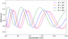 |
Fig. 3 Reflectance spectra measured on the reduced analog (deposited on MgF2 substrate) with the TAMS goniometer module for different incident angles (θ = 10, 20, 30, and 40°). |
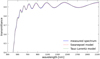 |
Fig. 4 Measured transmittance of the reduced analog deposited on a MgF2 substrate (blue curve) compared to the simulated spectrum of the Swanepoel method (pink curve) and Tauc-Lorentz model (green curve). The fitted parameters of the Tauc-Lorentz model are: A = 1.92 eV, C = 0.32 eV, Eo = 3.86 eV, Eg = 1.31 eV, and ε∞ = 2.34. The Swanepoel method and Tauc–Lorentz model predict a film thickness of 1375 and 1351 nm respectively. |
3.3 IR spectroscopy
3.3.1 Measurements
We performed IR measurements using a Bruker IFS125HR Fourier-Transform (FT) interferometric spectrometer at the AILES beamline of the SOLEIL synchrotron in Saint-Aubin (France). The sample compartment and optical system are put under a primary vacuum (~0.04 hPa) to avoid atmospheric contamination in the spectra. A silicon carbide Globar heated to 1250 K provides energy in the entire spectral range. Transmission spectra are acquired at an incident angle of 11°. In the MIR, we measure from 400 to 10 000 cm−1 with a step of 4 cm−1 using a KBr beam-splitter and an MCT detector cooled with liquid nitrogen. In the FIR, we measure from 100 to 400 cm−1 with a spectral resolution of 4 cm−1 using a 6-micron mylar beamsplitter with deposits of germanium and a bolometer detector cooled with liquid helium. Because of the low intensity of the source at FIR wavelengths and the lack of absorption with respect to our haze analog in that spectral region, the absolute transmission is less accurate. Therefore, we have limited our analysis of the FIR data to wavelengths below 30 µm.
The FT infrared spectroscopy does not operate in double-beam mode and therefore it does not provide absolute transmission directly. A reference spectrum without the sample is thus required to retrieve the baseline. Baseline correction alone is very sensitive and therefore introduces large errors in the absolute transmission unless we perform an additional reliable correction. As a second correction, we scaled our spectra to the absolute transmission obtained with spectrophotometry at the amine band (around 3.1 µm) where both measurements overlap. We used a similar scaling factor for the substrate spectrum. This scaling factor could also be obtained by comparing the measured transmission of the MgF2 with a simulated transmission since the optical constants of MgF2 are known. Both corrections provide similar results. For the sample deposited on the intrinsic Si substrate, the correction was also performed using the known optical properties of Si. In the FIR, interference fringes caused by multiple reflection within the 300-µm thick Si substrate were also removed following the procedure in Swanepoel (1983). This sample is used as the substrate is transparent in the MIR and FIR whereas the MgF2 substrate limits our measurement below 6–7 µm. The transmission of the reduced analog deposited on the Si substrate from 1.5 to 30 µm is shown in Fig. 5.
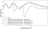 |
Fig. 5 MIR-FIR transmission of the reduced analog (blue curve) deposited on the intrinsic Si substrate. The first absorption-free transmission used as a baseline for Beer-Lambert calculation is shown in black. The updated baselines generated by the SSKK iteration model are shown, only three iterations are required to reach the chosen tolerance. |
3.3.2 Calculations
The extinction coefficient of the film (kf) is derived from the absolute transmission using a Beer-Lambert model that considers a coherent multiple reflection within the film:

where Tfs and To are, respectively, the measured transmittance and the simulated absorption-free transmittance of the film-substrate sample. In this calculation of k, the optical path accounts for the 11° incident angle used during the measurements.
Using the first-order Cauchy fit of the refractive index and the film thickness from the Swanepoel method, a first simulated absorption-free transmission To (assuming kf = 0, black curve in Fig. 5) can be calculated from Eq. (4). This initial calculation assumes a refractive index rather constant in the IR to calculate kf. This approach provides more accurate kf values in the MIR as we account for the coherent behavior of the film, rather than assuming To = Ts.
Using these first estimations of kf, we can more accurately calculate nf to satisfy Kramers-Kronig causality. A singly-substractive Kramers-Kronig (SSKK) algorithm is used to derive the refractive index in the IR. The KK equation in Eq. (1) shows us that the refractive index can in principle be calculated as a function of wavelength using n∞ and k(λ). Equation (1) can be rewritten to scale n in the entire range using an anchor point at a specific wavenumber (or wavelength), thereby replacing the ambiguous n∞ term. This expression, known as the singly substractive Kramers-Kronig equation, is expressed as follows (Hawranek et al. 1976):
![$ n\left( {{v_i}} \right) = {n_r} + {2 \over \pi }\left[ {P\int_0^\infty {{{vk(v)} \over {{v^2} - v_i^2}}\,} dv - P\int_0^\infty {{{vk(v)} \over {{v^2} - v_r^2}}dv} } \right]\,, $](/articles/aa/full_html/2024/02/aa46820-23/aa46820-23-eq12.png)
where nr and νr are the anchor point refractive index and wavenumber (cm−1), respectively.
In practice, the anchor value of nf was taken from the prediction of the Swanepoel method (see Sect. 3.2.2). For our calculations, we used the value of nf at 2000 nm. The accuracy of the anchor point is critical as it will be the main source of error propagating in the entire range (Hawranek & Jones 1976). As the integrands in Eq. (11) are not defined across the entire range of frequencies, we calculated the Cauchy principal value using Maclaurin s formula that was found to be the most reliable method (Ohta & Ishida 1988).
As more reliable n values can be retrieved for the film in the IR, a new simulated absorption-free spectrum was derived (see Fig. 5) and k was re-calculated with the Beer-Lambert equation. This iterative procedure was performed until the mean variation of k between two successive iterations becomes ≤1%. In practice, three iterations are sufficient, the main change occurs at the first iteration, around 6 µm where n changes significantly in response to the strong hetero-aromatic features. This iterative method prevents the propagation of interference fringes in the k spectra. We present and discuss these results in Sect. 5.
3.4 UV-Vis ellipsometry
3.4.1 Measurements
In standard ellipsometry, we measure the ratio of specular reflectance between parallel (p) and perpendicular (s) polarization. In polar coordinates, we express it as follows:

where Ψ and ∆ are the ellipsometric angles representing the amplitude ratio and phase difference, respectively.
We performed ellipsometric measurements from 300 to 830 nm using a Jobin-Yvon UVISEL ellipsometer at the LPICM (Laboratoire de Physique des Interfaces et des Couches Minces) laboratory, in Palaiseau (France). The operating principle of the ellipsometer is illustrated in Fig. 6. Radiation produced by the halogen lamp is transmitted through an optical fiber to then reach the polarization state generator (PSG) made of a simple linear polarizer. This specific type of instrument does not use a modulator (or retarder) on the PSG. The beam width can be adjusted at the exit of the PSG to reduce the spot size on the sample. A grazing geometry of 70° is used for reflection on the sample. The reflected beam then transfers through the polarization state analyzer (PSA) consisting of a photo-elastic modulator followed by a linear polarizer. This specific instrument is called a phase-modulated ellipsometer. The photo-elastic modulator is a material (fused silica) that exhibits birefringence upon mechanical stress, thus creating a phase difference as light splits and is transmitted through its different optical axes. The beam is spectrally resolved following the PSA. A photo-multiplier detector is used for this optical range.
The azimuths of the linear polarizers (P for the PSG and A for the PSA) and modulator (M) were set, while wo configurations are used to retrieve the ellipsometric angles ∆ and Ψ: P = 45°, M = 0°, A = 45° and P = 45°, M = 45°, and A = 90°.
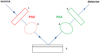 |
Fig. 6 General principles of our ellipsometric measurements: (1) and (5) are the linear polarizers of the polarization state generator (PSG) and polarization state analyzer (PSA) respectively; (2) and (4) are the modulators of the PSG and PSA respectively; (3) is the sample described in Fig. 1. |
3.4.2 Optical models
In ellipsometry, the spectral dispersion of the dielectric constant (Sect. 3.1.2) is expressed using parameterized functions which are derived from the various theoretical descriptions of dielectric polarization. For the present study, a non-exhaustive list of functions were used. We emphasize that several other descriptions exist and their validity mainly depends on the optical range as we move from electronic to atomic polarization.
For ellipsometric measurements, we used the doped Si sample (Table 1). Silicon is highly reflective, thus it efficiently enhances the sensitivity of our measurements. The dielectric function of the Si substrate is well-known in the UV–Vis range and therefore used as an input parameter. Reflection at the back of the substrate is negligible given the opacity of Si and the rugged back surface of our wafer. Therefore, the substrate was modeled as an infinite medium.
For the haze analog (film), we used three different dielectric functions, described below. The aim is to assess the accuracy of the retrieved optical constants using these different descriptions.
In the UV–Vis range, it is common to use the Tauc–Lorentz description to quantify absorption near the bandgap. The bandgap energy marks the onset of UV absorption in response to electronic polarization. The Tauc–Lorentz function expresses the imaginary part of the dielectric constant (ε2, see Sect. 3.1.2) as the product of Tauc’s equation with the classical Lorentz oscillator (Tauc et al. 1966; Campi & Coriasso 1988):

where E is the energy (eV), Eg is Tauc's bandgap energy (eV). Then, A, Eo, and C are the strength (eV), peak energy (eV), and width (eV) of the Lorentz oscillator, respectively.
It efficiently reproduces the extinction slope near the bandgap although it is not valid at lower energies (higher wavelengths). The real part of the dielectric constant is derived to satisfy the Kramers-Kronig relation (Jellison & Modine 1996).
As ε2 (or k) approaches 0, the Tauc–Lorentz formalism is reduced to an expression of n as a power law known as the Sellmeier equation:

where K is a constant and λ0 a constant wavelength (in µm).
Although this description assumes k = 0 in the spectral range of interest, it still considers absorption at lower wavelengths and its forcing on the spectral dispersion of n in the optical and UV range. We use this description in practice to retrieve df and nf in the transparent spectral region of the analog film.
The absorbent Cauchy description can also be used to reproduce the onset of absorption at optical and UV wavelengths. It conveniently provides estimations of k below the bandgap but lacks a physical meaning compared to the Tauc–Lorentz description. The absorbent Cauchy functions are expressed as follows:

where B, C, D, E, and F are constants. The units of these parameters can be deduced easily to ensure that n and k are dimensionless.
The dielectric function of our reduced haze analog is first expressed using a transparent Sellmeier model in the spectral region between 600 and 830 nm. Absorption by our haze analog is negligible in this optical window providing reliable estimations of the film thickness, df, and refractive index, nf. The dielectric function is then expressed following the Tauc–Lorentz and absorbent Cauchy descriptions in the entire spectral range from 300 to 830 nm.
The data analysis was performed using the Horiba DeltaPsi2 commercial software. The optical constants and film thickness of the haze analog are retrieved using iterative least-square fitting between our experimental data and the theoretical model. The model uses Ic and Is as fitting quantities and they are expressed using the ellipsometric angles as cos (2Ψ) cos (∆) and cos (2Ψ) sin (∆), respectively. The quality of the fit is described by the square residual:
![$ {\chi ^2} = \sum\limits_j {\left[ {{{\left( {I_{\rm{c}}^{{\rm{theo}}} - I_{\rm{c}}^{{\rm{exp}}}} \right)}^2} + {{\left( {I_{\rm{s}}^{{\rm{theo}}} - I_{\rm{s}}^{{\rm{exp}}}} \right)}^2}} \right]} , $](/articles/aa/full_html/2024/02/aa46820-23/aa46820-23-eq17.png)
where the summation over j refers to the number of data points.
The fit of experimental data with the three different models is shown in Fig. 7. The fitted parameters and square residuals are given in the caption. We present and discuss the retrieved optical constants in Sect. 4.2.
3.5 MIR ellipsometry
3.5.1 Measurements
The measurements used in this study were performed at the SMIS beamline of the SOLEIL synchrotron, in Saint-Aubin (France), using Mueller ellipsometry. The optical system of the Mueller ellipsometer is described in detail in Garcia-Caurel et al. (2015). The SiC Globar light source is provided by a Jobin Yvon FTIR spectrometer. The layout of the optical system is similar to the phase-modulated ellipsometer (Sect. 3.4.1), with an additional retarder on the PSG (as illustrated in Fig. 6). The PSG consists of a linear polarizer followed by a rhombohedric ZnSe retarder. Multiple reflections within the two ZnSe prisms create an achromatic retardation that elliptically polarizes the beam before reflection on the sample at angle of 60.5°. The PSA is similar to the PSG with the optical components in a reversed order. The retarders of the PSG and PSA are mounted onto mobile holders to change the azimuth and create different polarization states. The optical path ends with a MCT detector cooled with liquid nitrogen.
The standard ellipsometry previously used in the UV–Vis range is based on the Jones formalism that only stands for fully polarized light. The Stokes-Mueller formalism however applies for any polarization state including partial polarization. In this case, the polarization state of the beam is characterized using the Stokes vector as follows:

where x and y are two linear and orthogonal polarization states, while L and R refer to left and right circular polarization respectively. Also,  and
and  refer to two other linear polarization states.
Reflection on the sample introduces a linear transformation of the Stokes vector that can be retrieved from the measured intensities (Azzam 1977). It is the basic principle of Mueller ellipsometry that stands for any type of sample (isotropic or anisotropic). The linear coefficient of the transformation is expressed in the form of a 4 × 4 matrix called the Mueller matrix that satisfies the following condition:

where S is the Stokes vector preceding (Sp) and following (Sf) reflection on the sample, while M is the Mueller matrix.
The Mueller matrix holds the properties of the sample including optical constants and film thickness. In practice, 16 PSG-PSA configurations are required to retrieve every coefficient of the Mueller matrix. We used four azimuths for the PSG and PSA retarders. In other words, each of the four polarization states generated by the PSG and transformed by the sample is analyzed by four configurations of the PSA. We performed a calibration of the optical system to measure the Stokes vector of the PSG and PSA for each azimuth used. We thus obtained two matrices of Sp (Eq. (18)) and directly measured a 4 × 4 matrix of intensities from the 16 PSG-PSA configurations. Using this approach, the Mueller matrix is easily recovered using an algebraic matrix inversion.
For an isotropic sample, the Mueller matrix becomes solely function of the ellipsometric angles (Garcia-Caurel et al. 2013, 2015):

The isotropic nature of the sample is therefore inferred directly if our experimental Mueller coefficients satisfy the diagonal form in Eq. (19). We can see that the Mueller coefficients can be written using Ic and Is only. In a manner similar to UV–Vis ellipsometry, we then fit our measured Ic and Is with a model to retrieve the optical constants of our haze analog.
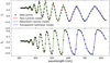 |
Fig. 7 Fit of the ellipsometric data in the UV–Vis range for the reduced haze analog (deposited on a doped Si substrate). The transparent Sellmeier model (blue curve) is only used between 600 and 830 nm as it assumes k = 0. The fitted Sellmeier parameters are: K = 2.569, λ0 = 138.2 µm and df = 1568.6 nm. The Tauc–Lorentz model is shown by the red curve, the fitted parameters are: ε∞ = 1.98, Eg = 2.01 eV, A = 10.58 eV, Eo = 5.88 eV, C = 2.52 eV and df = 1574.6 nm. The absorbent Cauchy model (green curve) fits best with n∞ = 1.619, D = 9.63E-3, E = −0.314 µm2, F = 1.148 µm4, B = 1.544 µm2, C = 0.21 µm4 and df = 1558.7 nm. The square residualsχ2 are 0.03, 0.15 and 0.25 respectively. |
3.5.2 Optical model
As we enter the range of atomic polarization, we go on to use different physical descriptions to parameterize the dielectric function. In the MIR and FIR, absorption is caused by free charge carriers and vibrations of chemical bonds.
Although the dielectric function of Si is well-known in principle, we used a P-doped substrate to increase its IR opacity and thus reduce reflection at the back of the wafer. The boron atoms diluted in the structure of the semiconductor create new energy states near the valence and conduction bands. As a consequence, the conduction band is reached around FIR frequencies. Absorption occurs as free electrons collide and scatter with the background of silicon atoms. The Drude description expresses the dielectric function on the basis of kinetic theory as follows:

where ω is the angular frequency (s−1), ωp is the plasma angular frequency (s−1), and Γ is a damping coefficient (s−1).
Therefore, we first performed measurements on our blank Si substrate to derive its optical properties affected by the concentration of boron atoms. The parameters of the Drude model are fitted (ωp and Γ), while only the plasma frequency is significantly changed as it is function of the dopant concentration. Once the dielectric function of our Si wafer is known, we use it as an input parameter for the analysis of the film-substrate sample.
Absorption by the haze analog results from bending and stretching of its covalent bonds. The Lorentz formalism describes resonant oscillations by assimilating electric dipoles to strings in a viscous fluid. Compared to gaseous molecules, the bonded structure of the material creates an opposite force to atomic oscillations quantified by a damping factor. For a complex material with several vibrational modes, the dielectric function is expressed using the sum of all classical oscillators. The Lorentz model only stands near the natural frequencies and cannot describe the intrinsic properties in the absence of absorption. The dielectric function is therefore scaled to its limit at inflnite frequency as follows:

where F, Eo, and D are the strength (eV), peak energy (eV) and width/damping (eV) of the oscillator, respectively. ε∞ is the dielectric constant at infinite wavenumber. The summation over j refers to the number of oscillators.
In the ellipsometric model, the different modes that mirror the composition of our haze analogs are fitted using Lorentz oscillators. The fitted parameters are: ε∞, df, the incident angle, and the constants of each oscillator (F, Eo, and D). The incident angle is known, in principle, but it might be slightly changed as we adjust the position of the sample. We therefore added this parameter in the fit, but constrained it to a 60–61° range.
Given the complexity of our material and the large number of stretching modes, the fit exhibits a strong degeneracy. Our main aim is to avoid reaching an unphysical numerical solution that would not accurately characterize the composition of the material. For that purpose, the natural frequencies (Eo) are kept constant, guided by our spectroscopic measurements (Fig. 5) and previous data on Titan haze analogs (Gautier et al. 2012; Mahjoub et al. 2012; Gavilan et al. 2018).
The deconvolution of hetero-aromatic features around 6–7 µm is difficult given the large number of overlapping modes (Gavilan et al. 2018). We simplified the picture of this region by using fewer oscillators to reduce the number of fitted parameters. Although it also prevents us from reaching a completely accurate physical description of the different modes, it still provides accurate estimations of kf. In this characterization of the reduced haze analog, we found that the sample was optimally fitted with nine oscillators. The fitted parameters are listed in Table 2. The orders of magnitude of these parameters are physically sensible for atomic vibrations although the strength and width of the 9th oscillator are unrealistically high. Here, the physical meaning of the last three oscillators is lost and only used to properly retrieve the continuum of k at FIR frequencies.
The fit of the Lorentz model to experimental data is shown in Fig. 8. We discuss the retrieved optical constants in Sect. 5.
Fitted parameters of the nine Lorentz oscillators.
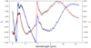 |
Fig. 8 Fit of MIR ellipsometric data for the reduced haze analog (deposited on a doped Si substrate). The best fit (χ2 = 4.32) suggests an incident angle of 60.48°, df = 1804 nm and ε∞ = 2.24 with nine oscillators. The fitted parameters of the oscillators are listed in Table 2. |
4 UV–Vis–NIR optical constants
4.1 Spectrophotometry
Using the goniometry method with different sets of reflectance spectra, the mean refractive index and film thickness were calculated in the NIR. We obtained a mean refractive index of 1.61, with an uncertainty of 0.09 (1σ) and a mean thickness of 1364 nm with an error of 76 nm (1σ). This simplest analytical approach provides an average estimation of n between 0.9 and 1.1 µm that can be used as an anchor point for SSKK integration. However, the uncertainty on n and d with this approach is high as the calculation solely considers the spectral shift of fringe extrema and ignores the height of the interference fringes. Thus, the method is sensitive to measurement biases that leads to high uncertainties. Given the high angular precision of the TAMS module, these errors likely emerge from the focalisation of the beam.
On the other hand, the Swanepoel method is proven to be extremely accurate. Indeed, the error between the measured and simulated spectra shown in Fig. 4 is below 0.4% above 500 nm. The extrapolation of n at lower wavelengths leads to higher uncertainties although the error remains below 1.5%. The film thickness is estimated at 1375 nm with a maximum error below 1% (Table 1). It confirms the expected accuracy retrieved on simulated spectra in Swanepoel (1983). As our optical model improves the construction of transmission envelopes using a tangent point method similar to Jin et al. (2017), the refractive index shown in Fig. 9 is analytically calculated in a large spectral range from 450 to 1500 nm. The low uncertainties on the thickness obtained by multiple measurements (Table 1) point to similarly reliable estimations of the refractive index n.
The Swanepoel method has also been applied to the analog deposited on the intrinsic Si substrate although measurements are limited above 1 µm as the Si wafer becomes opaque at lower wavelengths. We find that the refractive index n estimated is similar, only a change in thickness is observed (see Table 1). It was previously suggested that variations in composition of the analog could arise from using substrates with different dielectric properties in the PAMPRE setup (Mahjoub et al. 2012). Our new result suggests that the composition is similar and we reaffirm this statement in Sect. 4.3 in the context of a comparison with UV absorption.
Different spectrophotometric calculations of k were performed for the reduced analog (deposited on MgF2 substrate) and the results are shown in Fig. 10 (top panel). We find that the analytical expression of the Swanepoel method (Eq. (9)) provides similar estimations of k compared to a Beer-Lambert law using the transmission of the substrate and the envelope of maxima (Eq. (10)). To evaluate the error on k in the transparent window of our haze analog, we used a point-by-point fitting of k using the measured transmission and the refractive index fitted from the Swanepoel method. With this approach, we observed oscillations in the k spectrum (Fig. 10, top panel), resulting from very small errors on n and d. The propagation of interference fringes in the k spectrum is very weak in our case, thereby confirming the accuracy of the Swanepoel method.
In order to assess the effect of the model on the retrieved optical constants, we used an iterative Tauc-Lorentz model on our spectrophotometric data similar to the one used on our UV–Vis ellipsometric data (described in Sect. 3.4.2). The simulated transmission that best fits our data with a Tauc–Lorentz model is shown in Fig. 4. The retrieved optical constants are shown in Fig. 9 (for n) and 10 (for k). Above the retrieved bandgap energy (below 650 nm), we find similar k values compared to the analytical calculations with the Swanepoel method. However, we note a 1% discrepancy on n and d between both models. This discrepancy can be explained by the strong correlation between n and d in the law of interference (Eq. (3)).
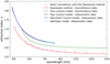 |
Fig. 9 Refractive index n of the reduced haze analog from UV to NIR retrieved with spectrophotometry on the MgF2 sample and ellipsometry on the doped Si sample. Direct calculations from transmission (purple data points) with the Swanepoel method are fitted to a Cauchy law (red curve). Indirect calculations with a Tauc–Lorentz model are performed on transmission data (green curve) and ellipsometric data (black curve). Also, n is retrieved using a Sellmeier model (cyan curve) and a Cauchy model (blue curve) on our ellipsometric data. |
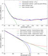 |
Fig. 10 Extinction coefficient, k, of the reduced haze analog from UV to NIR retrieved with spectrophotometry on the MgF2 sample and ellipsometry on the doped Si sample. Top: different spectrophotometric calculations of k from direct/analytical (Swanepoel, Beer-Lambert) and indirect/iterative (point-by-point fitting, Tauc–Lorentz) models. Bottom: measurements of k calculated using different models and different data (ellipsometric and spectrophotometric). The Swanepoel method shown on the bottom panel corresponds to the analytical expression on the top panel (red curve). |
4.2 Ellipsometry
The ellipsometric data were fitted to the Sellmeier, absorbent Cauchy, and Tauc–Lorentz models, as shown in Fig. 7. The retrieved optical constants are shown in Fig. 9 for n and 10 (bottom panel) for k. The models predict similar estimations of film thickness within a 20-nm error range (error below 1.5%). The thickness estimated at 1566 nm is thicker on the reduced haze analog deposited on Si substrate compared to the sample deposited on MgF2 substrate (see Table 1). This difference was previously observed (Gautier et al. 2012; Mahjoub et al. 2012) and is thought to result from the dielectric properties of the substrate and the position of the sample in the non-homogenous plasma discharge during the experiment.
From 600 to 830 nm, the Sellmeier model that assumes k = 0 provides similar n values compared to the Cauchy and Tauc–Lorentz models. At lower wavelengths, the Cauchy and Tauc–Lorentz models predict a similar spectral dispersion of n and similar k values. Therefore, the Cauchy model satisfies the Kramers–Kronig causality as well as the Tauc–Lorentz model, even though n and k were fitted with independent functions and parameters (see Eq. (15)). Although the Cauchy model is proven to be reliable, we are lacking a concrete physical meaning in the fitted parameters. Indeed, the k function of the Cauchy model is best fitted with a negative parameter. Both models are unable to quantify the weak absorption in the optical region. The Cauchy model indeed predicts negative values of k if not constrained, so the reliability of the predictions are lost in this optical range.
4.3 Spectrophotometry versus ellipsometry
We note a small discrepancy on the refractive index not only between both optical techniques, but also using a similar data set with a different model (Fig. 9). The discrepancy we see between both techniques is ~3% around 800 nm, which is generally lower than the variations observed by Tran et al. (2003). Two factors can explain this discrepancy: the strong anti-correlation between n and d seen with both methods, and the inhomogeneity of the film thickness. Indeed, our ellipsometric data in the optical region could still be fitted efficiently using different values of n and d. We also observed this correlation when comparing the Swanepoel method and Tauc–Lorentz model on our spectrophotometric data (Sect. 4.1). As for the second hypothesis, surface roughness does not improve the analysis on our ellipsometric data. Additionally, our spectrophotometric model is unable to converge to an estimation of roughness as the spectrum does not exhibit the shrinking of fringes expected for a non-homogeneous film. Therefore, we have several arguments suggesting that our estimations of n are not affected by the homogeneity of the film thickness. The small discrepancies in n are likely caused by its strong correlation with the film thickness. Given the small variations of n reported in the literature, we must be careful when comparing and correlating to the gas composition as these discrepancies might come from the measurements and calculations used.
In the UV, the different calculations provide extremely similar estimations of k with both data sets (Fig. 10, bottom panel). The high accuracy of both methods in this spectral range is expected given the large strength of UV features. Additionally, these new results support the statement in Sect. 4.1 asserting that the composition of the haze analog is similar for both the Si and MgF2 samples. Previous studies taught us that the change in gas composition lead to significant variations in the UV slope of k (Khare et al. 1984; Ramirez et al. 2002; Mahjoub et al. 2012; Jovanović et al. 2021; He et al. 2022). If changes in the composition were to be expected between the Si and MgF2 samples, changes in k would be observed in the UV.
The k values in the optical region could only be calculated with the Swanepoel method. We predicted an extinction coefficient close to 2–4.10−4 in agreement with previous measurements on Titan haze analogs (Khare et al. 1984; Ramirez et al. 2002; Imanaka et al. 2012). Our spectrophotometric estimations of k in that spectral range might be overestimated given the very small difference in transmission between the sample and substrate (Vuitton et al. 2009).
5 MIR optical constants: Spectrophotometry versus ellipsometry
The MIR extinction coefficients (k) calculated from Fouriertransform spectroscopy and Mueller ellipsometry are shown in Fig. 11. The general trend of k is similar between both methods and reflects the different vibrational modes characterizing our CHON haze analog. The different modes are described in detail in Gavilan et al. (2018) and categorized using the three following groups: amines (2.9–3.5 µm), nitriles (4.4–4.9 µm) and hetero-aromatics (5.8–8.3 µm). The oscillators used for the ellipsometric Lorentz model are attributed to the corresponding vibrational modes in Table 2. We note that IR reflection ellipsometry is not sensitive enough to efficiently detect weak absorption features as evidenced by the absence of C=H aliphatic (3.4 µm) or R–C≡N nitrile (4.5 µm) signatures observed in transmission.
Spectrophotometric and ellipsometric k values are very similar around the natural frequencies. We however observe variations in the inter-band regions as k is solely affected by the wings of the nearby oscillators. This discrepancy appears clearly in Fig. 11 on a logarithmic scale. In these inter-band regions, accurate estimations of k require a good knowledge of the structural order in the material. The ordered structure of semiconductors is very well described with the Lorentz oscillators. For more disordered isotropic material, the Kim oscillator conveniently allows the damping factor (Eq. (21)) to vary from Gaussian to Lorentzian. In Fig. 11, both descriptions provide similar estimations of k, although we notice a slight difference in the region between amine and nitrile absorption. The persisting discrepancy in terms of k compared to direct spectroscopic calculations stems from the use of a simplified Lorentz description with fewer oscillators to reproduce the hetero-aromatic features. Although this simplified model reduces the degeneracy, while maintaining a partially accurate physical description, it also forces the width of oscillators to increase, thereby overestimating the inter-band extinction coefficients. Indeed, the Lorentz model does not accurately fit the steep slopes separating nitrile and hetero-aromatic features observed in the ellipsometric data (Fig. 8) and confirmed in transmission spectroscopy (Fig. 5).
The Lorentz model predicts a film thickness d of 1804 nm (Fig. 8). The film thickness and thus the refractive index are significantly different than predictions with UV ellipsometry on a similar sample (Sect. 4.2). It suggests that the strong n-d correlation (discussed in Sect. 4.3) is not resolved in the Lorentz model because of a strong degeneracy with the fitted parameters of the oscillators. The discrepancies observed in the MIR inter-band regions can therefore also be caused by errors in n-d values leading to an incorrect correction of interference fringes that propagates in the k spectrum. Measurements in the Vis-NIR spectral range are therefore crucial to retrieve accurate n-d values and efficiently correct the effect of multiple reflection in the data analysis. Given the complexity of our material, we conclude that direct spectrophotometric calculations are more suited to retrieve accurate estimations of k in the MIR inter-band regions.
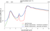 |
Fig. 11 MIR extinction coefficient of the reduced haze analog determined with spectroscopy on the MgF2 and intrinsic Si samples, and with Mueller ellipsometry on the doped Si sample. The different modes used for the ellipsometric Lorentz model are listed in Table 2. Gaussian and Lorentzian damping are considered to assess the impact on the interband k values. |
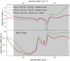 |
Fig. 12 Optical constants (n and k) measured from 0.3 to 30 µm on two exoplanet haze analogs. The analogs are produced from a 95% N2 gas mixture with different CO2 to CH4 ratios (see Table 1). The seminal data of Khare et al. (1984) for Titan haze analogs is shown in comparison. |
6 Optical constants in the spectral range of JWST: Implications for future observations
In Fig. 12, we report new optical constants from UV to FIR for exoplanet haze analogs. The refractive indices compiled in this work are available in the Optical Constants Database.
As we increase the CO2 to CH4 ratio, our measurements and calculations point to higher intrinsic IR absorption properties confirming previous finding by Gavilan et al. (2018). Additionally, the increased CO2 abundance in the gas phase results in a wider absorption peak regrouping hetero-aromatic modes around 6–8 µm. Additional work is required to assess the detectability of this strong feature in transit spectra. For the oxidized analog, we note that the slope of k on the high-frequency end of the hetero-aromatic group (around 6 µm) is shifted towards lower wavelengths compared to the reduced analog. This points to the presence of the C=O stretching band (at 5.8–5.9 µm) confirming the increasingly oxygenated nature of our exoplanet haze analogs. In the weakly absorbing NIR region, the extinction coefficient is similar for both analogs. The oxidized analog is less absorbing in the visible. In the UV, we note a stronger increase in the absorption slope for the oxidized analog, which might be caused by the presence of stronger high-energy UV features revealed in Gavilan et al. (2018).
We observe a significantly higher bandgap energy compared to Khare et al. (1984) that leads to variations of k by up to one order of magnitude in the Vis-NIR spectral range. In the MIR, our oxidized analog exhibits higher absorption compared to Khare et al. (1984). As shown by He et al. (2023), transit spectra are strongly affected by variations in the refractive indices of photochemical hazes. The data presented in this paper should therefore be used to interpret observations of CO2-rich rocky exoplanet atmospheres.
7 Conclusions
We comparatively assessed the accuracy of ellipsometric and spectrophotometric measurements to retrieve the optical constants of haze analogs. In the UV, k values are similar using both techniques. The variations of k between ellipsometric and spectroscopic calculations in the MIR are explained by the limitations of the Lorentz model. In the UV and MIR, the large variations of k reported in the literature largely overcome the error caused by the optical method and calculation. Thus, it likely results from the composition of the haze analogs although we cannot definitely conclude on the primary factor causing the change in composition as it can be caused by the gas composition or experimental conditions (residence time of the gas, pressure, temperature, etc.). We note a strong uncertainty in the k values with both techniques in the Vis-NIR as absorption is weak. We therefore expect this sensitivity to contribute significantly to the large discrepancies reported in the literature. As for the refractive index n, we find discrepancies of 1 to 3% between the different measurements and calculations at visible wavelengths. Small variations of n in the existing data could therefore stem from errors in the optical method and calculation. We confirm the strong accuracy of the Swanepoel method on our haze analogs in the UV–Vis–NIR. Reflection ellipsometry, however, constrains the dispersion of n at UV–Vis wavelengths more efficiently. Direct spectrophotometric calculations are preferred in the MIR region given the strong degeneracy observed in the analysis of ellipsometric data. We therefore recommend UV–Vis reflection ellipsometry to retrieve accurate values of refractive index and film thickness. This comparative optical study aims to guide the choice of future calculations and measurements to retrieve the refractive indices of exoplanet aerosol analogs.
Optical constants of haze analogs produced in a simulated N2-dominated/CO2-rich atmosphere are measured from 0.3 to 30 µm. We confirm the expected increased absorption for higher abundances of CO2. Our data predicts weaker absorption in the NIR and optical range compared to the first analogs of Khare et al. (1984). The different data sets obtained in a broad spectral range on haze analogs suggest strong variations of the optical properties, depending on the atmospheric composition. To better constrain retrieval models and correctly interpret future observations of oxidized exoplanet atmospheres, we encourage modelers to use these new data.
Acknowledgements
This work is supported by the “ADI 2021” project funded by the IDEX Paris-Saclay, ANR-11-IDEX-0003-02. T.D. and N.C. thank the European Research Council for funding via the ERC OxyPlanets project (grant agreement No. 101053033). T.G. acknowledges funding by ANR under the contract ANR-20-CE49-0004-01.
References
- Al-Ani, S. K. 2008, Iraqi J. Appl. Phys., 4 [Google Scholar]
- Alves, L. L., Marques, L., Pintassilgo, C. D., et al. 2012, Plasma Sources Sci. Technol., 21, 045008 [NASA ADS] [CrossRef] [Google Scholar]
- Arney, G., Domagal-Goldman, S. D., Meadows, V. S., et al. 2016, Astrobiology, 16, 873 [Google Scholar]
- Arney, G., Domagal-Goldman, S. D., Meadows, V. S. 2018, Astrobiology, 18, 311 [NASA ADS] [CrossRef] [Google Scholar]
- Ayupov, B. M., Sulyaeva, V. S., Shayapov, V. R., et al. 2011, J. Opt. Technol., 78, 350 [CrossRef] [Google Scholar]
- Azzam, R. M. A. 1977, Ellipsometry and Polarized Light (Elsevier North-Holland) [Google Scholar]
- Bakr, N. A., Funde, A. M., Waman, V. S., et al. 2011, Pramana, 76, 519 [NASA ADS] [CrossRef] [Google Scholar]
- Beichman, C., Benneke, B., Knutson, H., et al. 2014, PASP, 126, 1134 [NASA ADS] [CrossRef] [Google Scholar]
- Berry, J. L., Ugelow, M. S., Tolbert, M. A., & Browne, E. C. 2019, ApJ, 885, A6 [Google Scholar]
- Brassé, C., Muñoz, O., Coll, P., & Raulin, F. 2015, Planet. Space Sci., 109, 159 [CrossRef] [Google Scholar]
- Bruno, G., Lewis, N. K., Stevenson, K. B., et al. 2018, AJ, 155, 55 [NASA ADS] [CrossRef] [Google Scholar]
- Campi, D., & Coriasso, C. 1988, Mater. Lett., 7 [Google Scholar]
- De Kronig, R. L. 1926, J. Opt. Soc. Am. Rev. Sci. Instrum., 12, 547 [NASA ADS] [CrossRef] [Google Scholar]
- Deng, J., Du, Z., Karki, B. B., Ghosh, D. B., Lee, K. K. M. 2020, Nat. Commun., 11, 2007 [NASA ADS] [CrossRef] [Google Scholar]
- Dodge, M. J. 1984, Appl. Opt., 23, 1980 [NASA ADS] [CrossRef] [Google Scholar]
- Dorranian, D., Dejam, L., & Mosayebian, G. 2012, J. Theo. Appl. Phys., 6, 13 [NASA ADS] [CrossRef] [Google Scholar]
- El-Naggar, A. M., El-Zaiat, S. Y., & Hassan, S.M. 2009, Opt. Laser Technol., 41, 334 [NASA ADS] [CrossRef] [Google Scholar]
- Fujiwara, H. 2007, Spectroscopic Ellipsometry: Principles and Applications (Chichester: John Wiley & Sons Ltd) [CrossRef] [Google Scholar]
- Gaillard, F., & Scaillet, B. 2014, EPSL, 403, 307 [NASA ADS] [CrossRef] [Google Scholar]
- Gaillard, F., Bernadou, F., Roskosz, M., et al. 2022, EPSL, 577, 117255 [NASA ADS] [CrossRef] [Google Scholar]
- Gao, P., Thorngren, D. P., Lee, G. K. H., et al. 2020, Nat. Astron., 4, 951 [NASA ADS] [CrossRef] [Google Scholar]
- Gao, P., Wakeford, H. R., Moran, S. E., & Parmentier, V. 2021, J. Geophys. Res. Planets, 126, e2020JE006655 [CrossRef] [Google Scholar]
- Garcia-Caurel, E., De Martino, A., Gaston, J.-P., & Yan, L. 2013, Appl. Spectrosc., 67, 1 [NASA ADS] [CrossRef] [Google Scholar]
- Garcia-Caurel, E., Lizana, A., Ndong, G., et al. 2015, Appl. opt., 54, 2776 [NASA ADS] [CrossRef] [Google Scholar]
- Gautier, T., Carrasco, N., Mahjoub, A., et al. 2012, Icarus, 221, 320 [NASA ADS] [CrossRef] [Google Scholar]
- Gavilan, L., Broch, L., Carrasco, N., Fleury, B., & Vettier, L. 2017, ApJ, 848, L5 [NASA ADS] [CrossRef] [Google Scholar]
- Gavilan, L., Carrasco, N., Hoffmann, S. V., Jones, N. C., & Mason, N. J. 2018, ApJ, 861, 110 [NASA ADS] [CrossRef] [Google Scholar]
- Grigorovici, R., Stoica, T., & Vancu, A. 1982, Thin Solid Films, 97, 173 [NASA ADS] [CrossRef] [Google Scholar]
- Hawranek, J. P., & Jones, R. N. 1976, Spectrochim. Acta, 32A [Google Scholar]
- Hawranek, J. P., Neelakantan, P., Young, R. P., & Jones, R. N. 1976, Spectrochim. Acta, 32A [Google Scholar]
- Heng, K., Lyons, J. R., & Tsai, S.-M. 2016, ApJ, 816, 96 [NASA ADS] [CrossRef] [Google Scholar]
- He, C., Hörst, S. M., Lewis, N. K., et al. 2018a, ApJ, 856, L3 [CrossRef] [Google Scholar]
- He, C., Hörst, S. M., Lewis, N. K., et al. 2018b, ACS Earth Space Chem., 3, 39 [Google Scholar]
- He, C., Hörst, S. M., Radke, M., & Yant, M. 2022, Planet. Sci. J., 3, 25 [NASA ADS] [CrossRef] [Google Scholar]
- He, C., Radke, M., Moran, S. E., et al. 2023, Nat. Astron., in press, https://doi.org/10.1038/s41550-023-02140-4 [Google Scholar]
- Heng, K., & Showman, A. P. 2015, Annu. Rev. Earth Planet. Sci., 43, 509 [CrossRef] [Google Scholar]
- Hörst, S. M., He, C., Lewis, N. K., et al. 2018, Nat. Astron., 2, 303 [Google Scholar]
- Imanaka, H., Cruikshank, D. P., Khare, B. N., & McKay, C. P. 2012, Icarus, 218, 247 [NASA ADS] [CrossRef] [Google Scholar]
- Jellison, G. E., & Modine, F. A. 1996, Appl. Phys. Lett., 69, 371 [NASA ADS] [CrossRef] [Google Scholar]
- Jin, Y., Song, B., Jia, Z., et al. 2017, Opt. Express, 25, 31273 [NASA ADS] [CrossRef] [Google Scholar]
- Jovanović, L., Gautier, T., Vuitton, V., et al. 2020, Icarus, 346, 113774 [CrossRef] [Google Scholar]
- Jovanović, L., Gautier, T., Broch, L., et al. 2021, Icarus, 362, 114398 [CrossRef] [Google Scholar]
- Kawashima, Y., & Ikoma, M. 2018, ApJ, 853, 1 [NASA ADS] [CrossRef] [Google Scholar]
- Kawashima, Y., & Ikoma, M. 2019, ApJ, 877, 109 [NASA ADS] [CrossRef] [Google Scholar]
- Khare, B. N., Sagan, C., Arakawa, E. T., et al. 1984, Icarus, 60, 127 [CrossRef] [Google Scholar]
- Kitzmann, D., & Heng, K. 2018, MNRAS, 475, 94 [NASA ADS] [CrossRef] [Google Scholar]
- Kramers, M. H. A. 1927, Atti cong intern Fis. 2 [Google Scholar]
- Krissansen-Totton, J., Olson, S., & Catling, D. C. 2018, Sci. Adv., 4, eaao5747 [Google Scholar]
- Lacy, B. I., & Burrows, A. 2020, ApJ, 904, 25 [NASA ADS] [CrossRef] [Google Scholar]
- Lavvas, P., & Koskinen, T. 2017, ApJ, 847, 32 [NASA ADS] [CrossRef] [Google Scholar]
- Mahjoub, A., Carrasco, N., Dahoo, P.-R., et al. 2012, Icarus, 221, 670 [NASA ADS] [CrossRef] [Google Scholar]
- Mai, C., & Line, M. R. 2019, ApJ, 883, 144 [NASA ADS] [CrossRef] [Google Scholar]
- Manifacier, J. C., Gasiot, J., & Fillard, J. P. 1976, J. Phys. E: Sci. Instrum., 9, 1002 [NASA ADS] [CrossRef] [Google Scholar]
- Mikal-Evans, T. 2022, MNRAS, 510, 980 [Google Scholar]
- Moran, S. E., Hörst, S. M., Vuitton, V., et al. 2020, Planet. Sci. J., 1, 17 [NASA ADS] [CrossRef] [Google Scholar]
- Morley, C. V., Fortney, J. J., Marley, M. S., et al. 2015, ApJ, 815, 110 [NASA ADS] [CrossRef] [Google Scholar]
- Nuevo, M., Sciamma-O'brien, E., Sandford, S. A., et al. 2022, Icarus, 376, 114841 [NASA ADS] [CrossRef] [Google Scholar]
- Ohta, K., & Ishida, H. 1988, Appl. Spectrosc., 42, 852 [NASA ADS] [Google Scholar]
- Ozharar, S., Akcan, D., & Arda, L. 2016, J. Optoelectron. Adv. Mater., 18 [Google Scholar]
- Perrin, Z., Carrasco, N., Chatain, A., et al. 2021, Processes, 9, 965 [CrossRef] [Google Scholar]
- Pinhas, A., & Madhusudhan, N. 2017, MNRAS, 471, 4355 [Google Scholar]
- Ramirez, S. I., Coll, P., da Silva, A., et al. 2002, Icarus, 156, 515 [NASA ADS] [CrossRef] [Google Scholar]
- Rannou, P., Cours, T., Le Mouélic, S., et al. 2010, Icarus, 208, 850 [NASA ADS] [CrossRef] [Google Scholar]
- Reizman, F. 1965, J. Appl. Phys., 36, 3804 [NASA ADS] [CrossRef] [Google Scholar]
- Sciamma-O’Brien, E., Carrasco, N., Szopa, C., Buch, A., & Cernogora, G. 2010, Icarus, 209, 704 [CrossRef] [Google Scholar]
- Sciamma-O’Brien, E., Dahoo, P.-R., Hadamcik, E., et al. 2012, Icarus, 218, 356 [CrossRef] [Google Scholar]
- Sciamma-O'Brien, E., Upton, K. T., & Salama, F. 2017, Icarus, 289, 214 [CrossRef] [Google Scholar]
- Sing, D. K., Fortney, J. J., Nikolov, N., et al. 2016, Nature, 529, 59 [Google Scholar]
- Stenzel, O., Hopfe, V., & Klobes, P. 1991, J. Phys. D: Appl. Phys., 24, 2088 [NASA ADS] [CrossRef] [Google Scholar]
- Swanepoel, R. 1983, J. Phys. E: Sci. Instrum., 16, 1214 [NASA ADS] [CrossRef] [Google Scholar]
- Swanepoel, R. 1984, J. Phys. E: Sci. Instrum., 17, 896 [NASA ADS] [CrossRef] [Google Scholar]
- Szopa, C., Cernogora, G., Boufendi, L., Correia, J. J., Coll, P. 2006, Planet. Space Sci., 54, 394 [NASA ADS] [CrossRef] [Google Scholar]
- Tauc, J., Grigorovici, R., & Vancu, A. 1966, Phys. Stat. Sol., 15, 627 [CrossRef] [Google Scholar]
- Tian, M., & Heng, K. 2023, ArXiv e-prints [arXiv:2301.10217] [Google Scholar]
- Tompkins, H. G., & Irene, E. A. 2005, Handbook of Ellipsometry (William Andrew Inc.) [CrossRef] [Google Scholar]
- Tran, B. N., Joseph, J. C., Ferris, J. P., Persans, P. D., & Chera, J. J. 2003, Icarus, 165, 379 [NASA ADS] [CrossRef] [Google Scholar]
- Vuitton, V., Tran, B. N., Persans, P. D., & Ferris, J. P. 2009, Icarus, 203, 663 [NASA ADS] [CrossRef] [Google Scholar]
- Wakeford, H. R., & Sing, D. K. 2015, A & A, 573, A122 [Google Scholar]
- Woitke, P., Herbort, O., & Helling, C. 2021, A & A, 646, A43 [NASA ADS] [CrossRef] [EDP Sciences] [Google Scholar]
- Zellem, R. T., Swain, M. R., Cowan, N. B., et al. 2019, PASP, 131, 094401 [NASA ADS] [CrossRef] [Google Scholar]
All Tables
All Figures
|
Fig. 1 Haze analog: Thin film (ƒ) overlaying a substrate (s). Each medium (or layer) is characterized by its thickness (d) and complex refractive index (N). df ≪ ds in practice, the scale is changed for clarity. The measured reflection and transmission of the film-substrate sample, Rfs and Tfs, respectively, are affected by multiple reflections at the different interfaces. |
| In the text | |
|
Fig. 2 Measured transmittance of the reduced analog deposited on a MgF2 substrate (Tfs, blue curve). The transmission of the substrate alone is shown with the black curve. The transmission envelopes (TM and Tm) and the interference-free transmission (Tα) are constructed based on the Swanepoel method. |
| In the text | |
|
Fig. 3 Reflectance spectra measured on the reduced analog (deposited on MgF2 substrate) with the TAMS goniometer module for different incident angles (θ = 10, 20, 30, and 40°). |
| In the text | |
|
Fig. 4 Measured transmittance of the reduced analog deposited on a MgF2 substrate (blue curve) compared to the simulated spectrum of the Swanepoel method (pink curve) and Tauc-Lorentz model (green curve). The fitted parameters of the Tauc-Lorentz model are: A = 1.92 eV, C = 0.32 eV, Eo = 3.86 eV, Eg = 1.31 eV, and ε∞ = 2.34. The Swanepoel method and Tauc–Lorentz model predict a film thickness of 1375 and 1351 nm respectively. |
| In the text | |
|
Fig. 5 MIR-FIR transmission of the reduced analog (blue curve) deposited on the intrinsic Si substrate. The first absorption-free transmission used as a baseline for Beer-Lambert calculation is shown in black. The updated baselines generated by the SSKK iteration model are shown, only three iterations are required to reach the chosen tolerance. |
| In the text | |
|
Fig. 6 General principles of our ellipsometric measurements: (1) and (5) are the linear polarizers of the polarization state generator (PSG) and polarization state analyzer (PSA) respectively; (2) and (4) are the modulators of the PSG and PSA respectively; (3) is the sample described in Fig. 1. |
| In the text | |
|
Fig. 7 Fit of the ellipsometric data in the UV–Vis range for the reduced haze analog (deposited on a doped Si substrate). The transparent Sellmeier model (blue curve) is only used between 600 and 830 nm as it assumes k = 0. The fitted Sellmeier parameters are: K = 2.569, λ0 = 138.2 µm and df = 1568.6 nm. The Tauc–Lorentz model is shown by the red curve, the fitted parameters are: ε∞ = 1.98, Eg = 2.01 eV, A = 10.58 eV, Eo = 5.88 eV, C = 2.52 eV and df = 1574.6 nm. The absorbent Cauchy model (green curve) fits best with n∞ = 1.619, D = 9.63E-3, E = −0.314 µm2, F = 1.148 µm4, B = 1.544 µm2, C = 0.21 µm4 and df = 1558.7 nm. The square residualsχ2 are 0.03, 0.15 and 0.25 respectively. |
| In the text | |
|
Fig. 8 Fit of MIR ellipsometric data for the reduced haze analog (deposited on a doped Si substrate). The best fit (χ2 = 4.32) suggests an incident angle of 60.48°, df = 1804 nm and ε∞ = 2.24 with nine oscillators. The fitted parameters of the oscillators are listed in Table 2. |
| In the text | |
|
Fig. 9 Refractive index n of the reduced haze analog from UV to NIR retrieved with spectrophotometry on the MgF2 sample and ellipsometry on the doped Si sample. Direct calculations from transmission (purple data points) with the Swanepoel method are fitted to a Cauchy law (red curve). Indirect calculations with a Tauc–Lorentz model are performed on transmission data (green curve) and ellipsometric data (black curve). Also, n is retrieved using a Sellmeier model (cyan curve) and a Cauchy model (blue curve) on our ellipsometric data. |
| In the text | |
|
Fig. 10 Extinction coefficient, k, of the reduced haze analog from UV to NIR retrieved with spectrophotometry on the MgF2 sample and ellipsometry on the doped Si sample. Top: different spectrophotometric calculations of k from direct/analytical (Swanepoel, Beer-Lambert) and indirect/iterative (point-by-point fitting, Tauc–Lorentz) models. Bottom: measurements of k calculated using different models and different data (ellipsometric and spectrophotometric). The Swanepoel method shown on the bottom panel corresponds to the analytical expression on the top panel (red curve). |
| In the text | |
|
Fig. 11 MIR extinction coefficient of the reduced haze analog determined with spectroscopy on the MgF2 and intrinsic Si samples, and with Mueller ellipsometry on the doped Si sample. The different modes used for the ellipsometric Lorentz model are listed in Table 2. Gaussian and Lorentzian damping are considered to assess the impact on the interband k values. |
| In the text | |
|
Fig. 12 Optical constants (n and k) measured from 0.3 to 30 µm on two exoplanet haze analogs. The analogs are produced from a 95% N2 gas mixture with different CO2 to CH4 ratios (see Table 1). The seminal data of Khare et al. (1984) for Titan haze analogs is shown in comparison. |
| In the text | |
Current usage metrics show cumulative count of Article Views (full-text article views including HTML views, PDF and ePub downloads, according to the available data) and Abstracts Views on Vision4Press platform.
Data correspond to usage on the plateform after 2015. The current usage metrics is available 48-96 hours after online publication and is updated daily on week days.
Initial download of the metrics may take a while.