| Issue |
A&A
Volume 680, December 2023
Solar Orbiter First Results (Nominal Mission Phase)
|
|
|---|---|---|
| Article Number | L7 | |
| Number of page(s) | 12 | |
| Section | Letters to the Editor | |
| DOI | https://doi.org/10.1051/0004-6361/202348120 | |
| Published online | 12 December 2023 | |
Letter to the Editor
Relativistic electron beams accelerated by an interplanetary shock
1
Department of Physics and Astronomy, University of Turku, 20500 Turku, Finland
e-mail: This email address is being protected from spambots. You need JavaScript enabled to view it.
2
LPC2E/CNRS, UMR 7328, 3A Avenue de la Recherche Scientifique, Orléans, France
3
Space Sciences Laboratory, University of California, Berkeley, CA, USA
4
The Blackett Laboratory, Department of Physics, Imperial College London, London, UK
5
Center for mathematical Plasma Astrophysics, Department of Mathematics, KU Leuven, Celestijnenlaan 200B, 3001 Leuven, Belgium
6
Queen Mary University of London, School of Physics and Astronomy, London, UK
7
The Johns Hopkins University Applied Physics Laboratory, Laurel, MD, 20723
USA
8
Swedish Institute of Space Physics, PO Box 537 751 21 Uppsala, Sweden
9
Institute of Experimental & applied Physics, Kiel University, 24118 Kiel, Germany
10
Heliophysics Science Division, NASA Goddard Space Flight Center, Greenbelt, MD, 20771
USA
Received:
1
October
2023
Accepted:
10
November
2023
Abstract
Context. Collisionless shock waves have long been considered to be among the most prolific particle accelerators in the universe. Shocks alter the plasma they propagate through, and often exhibit complex evolution across multiple scales. Interplanetary (IP) traveling shocks have been recorded in situ for over half a century and act as a natural laboratory for experimentally verifying various aspects of large-scale collisionless shocks. A fundamentally interesting problem in both heliophysics and astrophysics is the acceleration of electrons to relativistic energies (> 300 keV) by traveling shocks.
Aims. The reason for an incomplete understanding of electron acceleration at IP shocks is due to scale-related challenges and a lack of instrumental capabilities. This Letter presents the first observations of field-aligned beams of relativistic electrons upstream of an IP shock, observed thanks to the instrumental capabilities of Solar Orbiter. This study presents the characteristics of the electron beams close to the source and contributes to the understanding of their acceleration mechanism.
Methods. On 25 July 2022, Solar Orbiter encountered an IP shock at 0.98 AU. The shock was associated with an energetic storm particle event, which also featured upstream field-aligned relativistic electron beams observed 14 min prior to the actual shock crossing. The distance of the beam’s origin was investigated using a velocity dispersion analysis (VDA). Peak-intensity energy spectra were anaylzed and compared with those obtained from a semi-analytical fast-Fermi acceleration model.
Results. By leveraging Solar Orbiter’s high temporal resolution Energetic Particle Detector (EPD), we successfully showcase an IP shock’s ability to accelerate relativistic electron beams. Our proposed acceleration mechanism offers an explanation for the observed electron beam and its characteristics, while we also explore the potential contributions of more complex mechanisms.
Key words: acceleration of particles / plasmas / relativistic processes / shock waves
© The Authors 2023
 Open Access article, published by EDP Sciences, under the terms of the Creative Commons Attribution License (https://creativecommons.org/licenses/by/4.0), which permits unrestricted use, distribution, and reproduction in any medium, provided the original work is properly cited.
This article is published in open access under the Subscribe to Open model. This email address is being protected from spambots. You need JavaScript enabled to view it. to support open access publication.
1. Introduction
Shock waves are ubiquitous in space plasmas, and are the most prolific particle accelerators in most systems. They can be directly probed in the heliosphere, due to the presence of planetary bow shocks (created due to the planetary obstacles in the solar wind flow) and interplanetary shocks, which are driven by solar activity such as coronal mass ejections (CMEs). CMEs are large-scale eruptions of plasma and magnetic fields that travel away from the Sun; when their speed exceeds the information speed of the medium (i.e., the fast magnetosonic speed), shock waves are generated. While ion acceleration in such shocks has been extensively studied (Lee et al. 2012, and references therein), electron acceleration is challenging due to the large separation in scales1 and physical limitations, such as their retention at the shock and magnetization (for a review, see Lembege et al. 2004). However, observational surveys have found a small number of interplanetary (IP) shocks that were associated with a significant increase in electron fluxes from subrelativistic to relativistic energies (e.g., Sarris & Krimigis 1985; Lopate 1989; Dresing et al. 2016; Mitchell et al. 2021; Talebpour Sheshvan et al. 2023). Furthermore, a strong correlation was found between the characteristics of relativistic ions and electrons, suggesting potential similarities in their acceleration mechanisms (Posner 2007; Dresing et al. 2022). While the acceleration of subrelativistic electrons (< 10 keV) by IP shocks is widely acknowledged, due to the common occurrence of type II radio emissions (Krasnoselskikh et al. 1985; Bale et al. 1999; Cairns et al. 2003; Jebaraj et al. 2020, 2021; Kouloumvakos et al. 2021), the acceleration of relativistic electrons (> 300 keV) by IP shocks remains an open question.
The characteristics and dynamics of collisionless shock waves are complex and are defined across multiple scales (Galeev & Karpman 1963; Karpman 1964; Sagdeev 1966; Kennel et al. 1985; Krasnoselskikh et al. 2013). These complexities are further enhanced when addressing the behavior of electrons at shock fronts (Balikhin et al. 1989; Trotta & Burgess 2019; Agapitov et al. 2023). An important property of shocks is their geometry, that is the angle between the upstream magnetic field (B) and the shock normal ( ), θBn. Quasi-perpendicular shocks (θBn > 45°) are often considered more efficient in accelerating electrons to high energies (Schatzman 1963; Bulanov et al. 1990; Mann et al. 2009). The typical widths of these shocks are larger than the electron gyro-radius (Walker et al. 1999; Hobara et al. 2010), and therefore their rapid acceleration can be explained via two main mechanisms. The first is the “fast-Fermi” process, where acceleration happens via magnetic mirroring (due to the steep magnetic gradient at quasi-perpendicular shocks, Leroy & Mangeney 1984; Wu 1984). This mechanism has been exploited for almost four decades when discussing the field-aligned beams (FABs) of energetic particles (e.g., Pulupa & Bale 2008). The second process is a gradient drift mechanism commonly known as shock-drift acceleration (SDA; Hudson 1965; Ball & Melrose 2001) which is similar to fast-Fermi acceleration, but deviates due to electron drift along the small-scale electric field gradients within the shock ramp (Krasnoselskikh et al. 2002; Vasko et al. 2018; Dimmock et al. 2019; Hanson et al. 2020).
Spacecraft upstream of the terrestrial bow shock have routinely measured 10 − 100 keV (near-relativistic electrons; e.g., Wilson et al. 2016) and far higher energy electrons at other planetary bow shocks, such as those of Jupiter and Saturn (e.g., Masters et al. 2017). The most frequently observed similarity in conditions across all these planetary bow shock observations is the presence of a shock that has exceeded a certain critical point beyond which the downstream sound speed (cs) is greater than the flow speed. Such shocks are termed super-critical, and behave fundamentally differently from those where cs is slower than the flow speed downstream, which are known as sub-critical. This is characterized best by the ratio of the shock speed to the fast magnetosonic speed known as the Mach number M. Super-critical shocks are usually strong shocks, while sub-critical are weak shocks. Depending on the shock geometry, super-critical shocks can generate ion-kinetic structures in the region ahead of the shock (foreshock), which trap and energize particles (Kennel 1981; Kis et al. 2013). However, observations of electron trapping and energization are rare in IP shock waves, which are generally weak shocks (Armstrong & Krimigis 1976; Sarris & Krimigis 1985; Shimada et al. 1999). Super-critical shocks may also be crucial for ion acceleration and may be the reason for the good correlations between relativistic ions and electrons at strong coronal shocks (Kouloumvakos et al. 2019; Dresing et al. 2022).
In this study we present measurements of relativistic electron beams found upstream of a traveling shock wave driven by an IP coronal mass ejection (ICME). To our knowledge, this is the first such study made possible thanks to the enhanced time resolution (1 s) of the Energetic Particle Detector (EPD; Rodríguez-Pacheco et al. 2020) instrument suite on board Solar Orbiter (SolO; Müller & Marsden 2013). We utilized the Electron Proton Telescope (EPT) which covers electron energy in the range ≈30 keV–300 keV, and the High Energy Telescope (HET) which covers > 400 keV. The Letter is structured as follows. An overview of the event is presented in Sect. 2, experimental details of the FABs and a demonstration of their origin from a remote location of the shock are presented in Sect. 3.1, and a robust peak-intensity spectral analysis in Sect. 3.2. Finally, a simple shock acceleration model for FABs is presented in Sect. 4, and the results and its implications in Sect. 5.
2. Overview of the in situ shock and associated energetic electrons
On 25 July 2022, at 06:22:45 UT, the SolO spacecraft encountered an IP fast-forward shock wave (see the last three panels of Fig. 1). It was linked to a weak C1 solar flare and CME on 23 July 2022 at about 18:30 UT. A remarkable aspect related to the in situ shock crossing (first two panels of Fig. 1, and Fig. A.1), is the presence of upstream field-aligned beams of relativistic electrons (up to ∼1 MeV) indicated by the gray shaded region. The shock was also associated with an energetic storm particle (ESP) event for electrons, whose features are outside the scope of this Letter, but a short summary is provided in Appendix A.
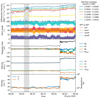 |
Fig. 1. Overview of the in situ shock and energetic electrons observed by Solar Orbiter on 25 July 2022. The arrival of the shock at 06:22:47 is indicated by the vertical gray dashed line in all panels. The first panel shows the differential intensities of energetic electrons observed by the south telescopes of EPT and HET (covering a stable pitch angle of 180° throughout the shown period). The upstream FABs are observed between 06:06:00 and 06:08:30 UT, and are indicated by the gray shaded region. Figure A.1 shows the differential intensities across all viewing directions. The second panel presents the pitch-angle coverage for the different viewing directions of EPT and HET, where the gradients in color indicate the different telescope openings of EPD/EPT (smaller) and EPD/HET (larger). The third and fourth panels show the components of the magnetic field, and bulk flow velocity, while the fifth panel presents the ion number density and proton temperature. |
The shock arrived at SolO approximately 36 hours after the solar event, which results in an average transit speed of 1100 km s−1. In order to obtain the in situ characteristics of the shock wave, such as its speed and strength, a more robust physical approach involving multiple steps was adopted.
First, the shock normal ( ) was estimated using a combination of the mixed-mode method, magnetic and velocity coplanarity (Trotta et al. 2022, and references therein), and minimum variance analysis (MVA; Sonnerup & Scheible 1998) to be
 ![Mathematical equation: $ \hat{\boldsymbol{n}} = [0.93 \pm 0.05, 0.018 \pm 0.12, -0.16 \pm 0.25] $](/articles/aa/full_html/2023/12/aa48120-23/aa48120-23-eq3.gif) . Next, the shock’s obliquity was estimated to be θBn ∼ 64° ±6°, indicating a quasi-perpendicular geometry. The upstream and downstream bulk flow speeds were then estimated in the shock rest frame,
. Next, the shock’s obliquity was estimated to be θBn ∼ 64° ±6°, indicating a quasi-perpendicular geometry. The upstream and downstream bulk flow speeds were then estimated in the shock rest frame,  km s−1 and
  km s−1, which results in a shock speed, Vsh ∼ 775 ± 50 km s−1 in the observers frame. The Alfvén Mach number (MA) was then estimated using the upstream Alfvén speed,
  (assuming Z = 1, mi and ni are proton mass and number density), and proxies (for MA) established in Gedalin et al. (2021) to be MA ∼ 3.3 ± 0.7. Single spacecraft techniques to obtain shock parameters are cumbersome and may possess large uncertainties, and proxies act as constraints. Another indicator of the shock’s strength is its compression ratios: rB ∼ 3 for magnetic compression (Bdown/Bup) and rgas of at least ∼2.1 for gas compression (ndown/nup). The estimated rgas may be influenced by data uncertainties, and therefore for a quasi-perpendicular shock, based on the Rankine-Hugoniot relations, rgas is expected to be similar to rB. This uncertainty was also considered when estimating Vsh and MA.
3. Upstream field-aligned electron beams
3.1. Observational details and the properties of the electron beams
During the period of shock arrival (see Fig. 1), the pitch-angle (PA) coverage of EPD was unusually stable due to the very stable magnetic field vector. The orientation of the magnetic field was north–south, resulting in field-aligned anti-sunward propagating particles being detected in the south telescopes of the SolO/EPD instruments with PA close to 180°. Consequently, the north telescope measured particles propagating toward the Sun, while the sun and anti-sun telescopes covered particle PA perpendicular to the magnetic field (∼90°). Taking this into account, electron observations from only the south telescope are presented in the main text. Detailed observations from all telescopes can be found in Appendix A. Since the measured electron intensities may be subject to ion contamination, robust contamination corrections were applied using different techniques for EPT (Appendix A.1) and for HET (Appendix A.2) measurements.
The first panel in Fig. 1 presents the differential electron intensities observed by the south telescopes of EPT and HET post-correction, which show a clear increase in the electrons above the background. Thanks to the high time resolution provided by EPT and HET (full resolution is 1 s), it was possible to identify, for the first time, fine features, particularly electron FABs upstream of the shock between 06:06:00 and 06:08:30 UT (∼14 min prior to shock arrival) in the south-facing telescopes (indicated by the gray shaded region in Fig. 1). These FABs have never been clearly measured upstream of interplanetary shocks before, possibly due to the lack of sufficient time resolution of the particle measurements. On closer inspection, this particular FAB had two peaks within it, which are distinguishable over the same range of energies. Since the FABs were only observed by the south telescopes, and the lower-energy STEP telescope only has a field of view in the sunward direction, the FABs could not be observed at lower energies (subrelativistic, i.e., < 10 keV). However, Langmuir wave packets were registered by the Time Domain Sampler (TDS) instrument, which is a part of the Radio Plasma Waves (RPW; Maksimovic et al. 2020) instrument suite. Two wave packets (not shown), the first at 06:10:05 UT and then at 06:11:59 UT, is likely evidence of the FABs extending to subrelativistic energies. Other than small amplitude Langmuir waves, no strong wave activity was measured during this time, making it improbable that the FABs are generated locally. The presence of Langmuir waves also indicates the remote origin of the beam, as it must have propagated at a distance that is, at the very least, on the order of its relaxation length (Ryutov 1969; Voshchepynets et al. 2015; Jebaraj et al. 2023a).
Under the assumption that electrons of all energies were injected at the same time (e.g., Vainio et al. 2013), a velocity dispersion of the FABs allows the injection time and the propagated path length of the FABs to be estimated. The details of this analysis can be found in Appendix A.3. The results of the analysis shown in Fig. A.5 suggest that the electrons were accelerated in a region ∼13 R⊙ from the observer, and were injected at 06:05:46 UT.
3.2. Assessing the characteristics of electron acceleration using peak-intensity energy spectra
The generation and propagation of the FABs can be understood better by constructing a peak-intensity spectrum across all observed energy channels (e.g., Dresing et al. 2020). The two top panels of Fig. 2 present background-subtracted and contamination-corrected electron peak-intensity spectra of the two well-defined peaks within the FAB, using measurements from both EPT and HET south-facing telescopes and a time resolution of 15 s. Light gray markers represent the subtracted background, while the colored markers indicate the peak electron fluxes.
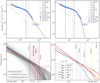 |
Fig. 2. Comparison of the peak-intensity electron spectra: observation (top) vs. model (bottom). In the top two panels the points in cyan signify the first peak, while points in blue denote the second peak. The corresponding fits are indicated by orange for the first peak and blue for the second. The background that has been subtracted from each energy channel is represented by points in gray. Top left: Broken power-law fits applied to both peaks. Top right: Broken power-law fits with an exponential roll-over (or cutoff) for the two peaks. Bottom left: Ensemble of runs indicated by the gray shaded region with varying κ ∼ 3 − 4 and θBn ∼ 87° −89.5°. A single power-law fit and exponential roll-over (blue dashed line), and a broken power-law fit (red dashed line) are shown for the modeled mean. The fit for the first peak from top left panel is illustrated by the olive-black dash-dotted line. The mean roll-over (Ec) and break energies (Eb) of the ensemble and its standard deviation are also shown. Bottom right: Modeled results using κ ∼ 3.5 for different θBn (88° −89.5°). The corresponding break energies are indicated by the vertical dashed lines. |
The method for spectral fitting outlined in Dresing et al. (2020), Strauss et al. (2020) allows for different fit models. For the FABs, we used a broken power law defined by two different spectral indices δ1 and δ2 separated at a break-energy Eb, a single power law (δ1) with an exponential roll-over or cutoff energy Ec, and a broken power law with an exponential roll-over at higher energies. Depending on the respective peak and the energy range taken into account in the fitting procedure, different models that fit the data were obtained. The top right panel of Fig. 2 shows the fit applied to both peaks over all available EPT channels, and therefore also fitting the ankle-like feature below 100 keV, which is more pronounced in the spectrum of the second peak than the first. The resulting fits both yield a similar exponential roll-over at higher energies. If the ankle is excluded from the fit, as done in Fig. 2 (top left), the fit results in a broken power law for both peaks. Although these fits seem to yield a better agreement with the HET points, it is hard to conclude what type of fit (either a broken power law or an exponential roll-over) is the best representation of the spectrum. This is, on the one hand, due to the HET electron peak fluxes potentially being subject to a small amount of proton contamination, which would lead to slightly increased fluxes, and, on the other hand, because the ion-contamination correction that was applied to the EPT data points was not perfect. The presence of a break or spectral roll-over is without doubt, as it is already evident in the uncorrected EPT data (not shown).
The cutoff energies Ec for both the fits in the right panel are similar, ∼200 keV. However, the break energies Eb for the fits in the left panel are both found to be above ∼200 keV, but are slightly different. The most significant difference in the two spectra was at lower energies, the second peak exhibits a more pronounced ankle at approximately ∼70 keV. The lower spectral index of the first peak in the right panel is δ = −1.19 ± 0.14, while that of the second peak is δ = −1.96 ± 0.54. For comparison, the spectral indices for the first peak in the left panel are δ1 = −1.66 ± 0.08 and δ2 = −5.69 ± 2.09, while that of the second peak are δ1 = −0.94 ± 0.06 and δ2 = −5.02 ± 0.79. We also fit an averaged spectrum of a time period of 2.5 min containing both peaks, which results in a broken power law with δ1 = −1.4 ± 0.04, δ2 = −5.2 ± 2.58, and Eb = 261.8 ± 47 keV (not shown).
4. A model for electron acceleration at IP shocks
From the observations presented in this Letter, it is understood that the FABs were accelerated at a remote location on the shock similar to how they are accelerated at the near-perpendicular terrestrial bow shock. If so, then the curvature of the shock (or large-scale deformations for the IP shock at 1 AU) and the time-varying properties of the upstream magnetic field become crucial. Acceleration happens under the exclusive assumption that there exists a region on the shock wave separated by ∼13 R⊙ that is near-perpendicular (89.9° > θBn > 85°) and super-critical2 (Appendix B). When these conditions are met, acceleration happens based on the conservation of magnetic moment (the fast-Fermi mechanism, Sonnerup 1969; Wu 1984; Leroy & Mangeney 1984) through which electrons can gain a significant amount of energy in a single encounter with a near-perpendicular shock.
The primary aspect of super-critical shocks is that in order to dissipate excess energy, they reflect a portion of upstream ions forming an overshoot magnetic field (Krasnoselskikh et al. 2013). The steep magnetic gradient of the overshoot enables the near-relativistic and relativistic electrons to conserve their magnetic moment and as such, a relativistic approach to the fast-Fermi mechanism must be adopted (Appendix B). We note that a sub-critical shock is also capable of reflecting electrons, but to a far lesser degree as far fewer particles would undergo such a process. The second important assumption is that in a near-perpendicular geometry, the shock speed along the magnetic field line scales as a function of geometry. This limits acceleration to only those particles that exceed it, resulting in dilute beams.
We performed semi-analytical modeling based on the relativistic form of the reflection conditions provided in Leroy & Mangeney (1984). When θBn > 89.5°, the shock speed must also undergo a Lorentz transformation as it is relativistic. The upstream seed electron distribution function was assumed to be a kappa-distribution (Appendix B) with κ ∼ 3 − 4 (considered realistic, Krauss-Varban & Burgess 1991). For the parameters of the shock, an upstream magnetic field similar to that measured in situ by SolO was used (i.e., ∼10 nT). The magnetic compression including the overshoot magnetic field is considered to be Bovershoot/B = 7 (based on Mellott & Livesey 1987) yielding a maximum B of 70 nT. Finally, the effect of the electrostatic potential cannot be ignored for electrons, and as such 100 eV was used (obtained through proxies, Appendix B).
The modeling results are presented in the bottom two panels of Fig. 2. An ensemble of runs was performed using kappa values in the range κ ∼ 3 − 4, and shock obliquity in the range θBn ∼ 87° −89.5°. The gray shaded region in the bottom left panel of Fig. 2 shows the results and two different fits to the mean of all runs, namely a single power law with a roll-over (blue dashed line) and a broken power law (red dashed line). The first has a power law with spectral index δ ∼ −2.4, which is followed by an exponential roll-over, while the second has two power laws with spectral indices δ1 ∼ −2.5 and δ2 ∼ −6.6. Both fits are used, but the χ2 of the first fit is lower than that of the second. The mean cutoff energy (Ec) for the first fit was ∼290 keV and the mean break-energy (Eb) of the second fit was ∼330 keV. The vertical red shaded region shows the 2σ standard deviation of both fits, which are similar. For comparison, the broken power law of the first peak (i.e., δ1 ∼ −1.66 and δ2 ∼ − 5.7, shown as the orange fit in top left panel of Fig. 2) from observations is represented in black. Both the modeled spectral indices and the break-energy range are comparable to the observations.
In a general sense, fast-Fermi acceleration simply shifts the seed distribution minus the transmitted electrons to higher energies (see Appendix B). This is also corroborated by the fact that a single power law with an exponential roll-over produces a better χ2 than a broken power-law fit. The mechanism does not change the shape of the source κ-distribution function. The shift (i.e., energy gain) itself is highly dependent on the shock obliquity, and this is clearly shown in the bottom right panel of Fig. 2. When κ = 3.5 is a fixed value and the obliquity is varied between θBn = 88° −89.5°, the resulting energy spectra are significantly different for energies above 100 keV. The difference is quantified by the dotted vertical lines representing the break energies (Eb) for each θBn. The effect of a changing κ index would then be responsible for the steepness of the spectrum since it determines the number of electrons in the tail. A κ = 2 can be characterized with a power-law index of δ ∼ −1.5 at suprathermal energies and an exponential roll-over above a certain energy range (Oka et al. 2018). Then, the steepest result possible is when the distribution tends toward a Maxwellian distribution as κ → ∞.
Finally, it is worth mentioning that the model used here makes two main simplifications, namely a 1D shock profile and that the electron’s magnetic moment is conserved. In reality, super-critical shocks are complex (Krasnoselskikh 1985; Lembege & Savoini 1992; Balikhin et al. 1997), and acceleration by multiple reflections and subsequent gradient drift (SDA) may also take place (see Appendix B for more details). In such cases the resultant distribution will deviate from what is presented here and may resemble a broken power law.
5. Discussion of the results
On 25 July 2022 a traveling IP shock wave accompanied by an energetic storm particle event was recorded in situ by Solar Orbiter. Notably, field-aligned beams of relativistic electrons were observed 14 min prior to the shock arrival. These are the first such observations of electron FABs measured at IP shocks thanks to the high temporal resolution of the EPD instrument suite on board SolO. This Letter presents their observational characteristics and proposes a scenario for their acceleration at IP shocks.
A combination of a lack of upstream magnetic structures, and the velocity dispersion of the FABs lead to the conclusion that they originated at a remote location of the shock. Velocity dispersion analysis suggested that the beams originated ∼13 R⊙ from the spacecraft. Further corroboration was provided by the presence of plasma waves (Langmuir waves, Filbert & Kellogg 1979; Kasaba et al. 2000), which are a consequence of beam propagation and relaxation (quasi-linear relaxation, Vedenov et al. 1963).
Galeev & Karpman (1963) initially postulated that shocks evolving in a low-density inhomogeneous plasma might develop decay instabilities that deform the laminar shock front. In higher dimensions, large-scale deformations lead to curved fronts on the scale of the upstream inhomogeneities, spanning from several R⊙ to tens of R⊙ (e.g., Wijsen et al. 2023), which play a significant role in FAB acceleration (Bulanov & Sakharov 1986; Decker 1990; Bulanov & Krasnoselskikh 1999; Lario et al. 2008). With any curved front, a finite region exists where θBn ≥ 85° and approaches 90°, allowing efficient electron acceleration along the tangent magnetic field line, as demonstrated in this Letter. When the observer is connected to the tangent field line, the time-varying properties of the FABs are likely influenced by deformation-induced curvature and by variations in the upstream field topology (e.g., Giacalone 2017; Trotta et al. 2023).
Similarities between the observed and modeled peak-intensity spectra of the FABs serve as a demonstration of shock acceleration at an IP shock under the right circumstances. The model naturally forms a roll-over or break at higher energies (> 200 keV), which is also seen in observations. If a broken power law were fit to the modeled results, the break-energy Eb would fall between 190 keV and 400 keV, comparable to the observations. This is considerably different from the transport-related breaks discussed in previous studies (Dresing et al. 2021), which have suggested that the presence of two different spectral breaks in peak-intensity spectra of solar energetic electron events are caused by transport-related effects. The spectral fits and the slopes obtained here are unique since it is the first such result obtained close to the source, that is, the IP shock. In particular, the spectral break observed at high energies (i.e., > 200 keV) reported for the first time here is therefore likely a direct consequence of acceleration.
The fast-Fermi and SDA mechanisms are both candidates for electron acceleration. The characteristics of these mechanisms depend on the conditions at the source, the seed distribution function, and the shock properties (e.g., obliquity, criticality). The solar wind conditions in reality are constantly changing, altering the conditions for acceleration, favoring a rapid mechanism. Furthermore, it is possible that electrons accelerated in such hot-spots can drift back onto the shock due to the E × B drift at large distances and can undergo further acceleration via a first-order Fermi process.
This Letter presents novel observations of relativistic electron beams and demonstrates the efficiency of IP shock acceleration of electrons at 1 AU. The results highlight the importance of shock geometry, large-scale deformations, and the resultant curvature in electron acceleration. This research paves the way for investigating similar phenomena closer to the Sun, where shock waves are inherently curved, predominantly near-perpendicular, and are in proximity to dense populations of energetic particles (Jebaraj et al. 2023b).
Ratio of gyro-radii (rL)  , where mi and me are the mass of protons and electrons, respectively.
When the downstream medium is subsonic (i.e., when the sound speed  ), the shock undergoes fundamental changes in its evolution and structure (Krasnoselskikh 1985).
Acknowledgments
I.C.J and N.D. are grateful for support by the Academy of Finland (SHOCKSEE, grant No. 346902). We also acknowledge funding by the European Union’s Horizon 2020 research and innovation program under grant agreement No. 101004159 (SERPENTINE). I.C.J acknowledges support from ISSI as part of the visiting scientist program. I.C.J, V.K, and O.V.A. acknowledge support from the International Space Science Institute (ISSI) in Bern, through ISSI International Team project number 23–575, “Collisionless Shock as a Self-Regulatory System”. V.K. acknowledges financial support from CNES through grants, “Parker Solar Probe”, and “Solar Orbiter”. V.K., and O.V.A. were supported by NASA grants 80NSSC20K0697 and 80NSSC21K1770. O.V.A was partially supported by NSF grant number 1914670, NASA’s Living with a Star (LWS) program (contract 80NSSC20K0218), and NASA grants contracts 80NNSC19K0848, 80NSSC22K0433, 80NSSC22K0522. A.L. is supported by STFC Consolidated Grant ST/T00018X/1. A.K. acknowledges financial support from NASA NNN06AA01C (SO-SIS Phase-E, PSP EPI-Lo) contract. N.W. acknowledges support from the Research Foundation – Flanders (FWO-Vlaanderen, fellowship no. 1184319N). D.L. acknowledges support from NASA Living With a Star (LWS) program NNH19ZDA001N-LWS, and the Goddard Space Flight Center Heliophysics Innovation Fund (HIF) program. I.C.J is grateful for the fruitful discussion with Dr. Jens Pomoell regarding IP shocks. Solar Orbiter is a space mission of international collaboration between ESA and NASA, operated by ESA. The open-source Python packages SEPpy (Palmroos et al. 2022), solo-epd-loader (Gieseler & Palmroos 2023), and sunpy (Barnes et al. 2023) have been used in obtaining and processing Solar Orbiter data.
References
- Agapitov, O. V., Krasnoselskikh, V., Balikhin, M., et al. 2023, ApJ, 952, 154 [NASA ADS] [CrossRef] [Google Scholar]
- Armstrong, T. P., & Krimigis, S. M. 1976, J. Geophys. Res., 81, 677 [NASA ADS] [CrossRef] [Google Scholar]
- Bale, S. D., Reiner, M. J., Bougeret, J. L., et al. 1999, Geophys. Rev. Lett., 26, 1573 [NASA ADS] [CrossRef] [Google Scholar]
- Balikhin, M. A., Krasnosel’Skikh, V. V., & Woolliscroft, L. J. C. 1989, Adv. Space Res., 9, 203 [NASA ADS] [CrossRef] [Google Scholar]
- Balikhin, M. A., Walker, S. N., de Wit, T. D., et al. 1997, Adv. Space Res., 20, 729 [NASA ADS] [CrossRef] [Google Scholar]
- Ball, L., & Melrose, D. B. 2001, PASA, 18, 361 [NASA ADS] [CrossRef] [Google Scholar]
- Barnes, W. T., Christe, S., Freij, N., et al. 2023, Front. Astron. Space Sci., 10, 1076726 [NASA ADS] [CrossRef] [Google Scholar]
- Bulanov, S. V., & Krasnoselskikh, V. 1999, in Magnetic Fields and Solar Processes, ed. A. Wilson, ESA Spec. Publ., 448, 1047 [NASA ADS] [Google Scholar]
- Bulanov, S., & Sakharov, A. 1986, JETP Lett., 44, 543 [NASA ADS] [Google Scholar]
- Bulanov, S., Kovrizhnykh, L., & Sakharov, A. 1990, Phys. Rep., 186, 1 [NASA ADS] [CrossRef] [Google Scholar]
- Cairns, I. H., Knock, S. A., Robinson, P. A., & Kuncic, Z. 2003, Space Sci. Rev., 107, 27 [NASA ADS] [CrossRef] [Google Scholar]
- Decker, R. B. 1990, J. Geophys. Res., 95, 11993 [NASA ADS] [CrossRef] [Google Scholar]
- Dimmock, A. P., Russell, C. T., Sagdeev, R. Z., et al. 2019, Sci. Adv., 5, eaau9926 [NASA ADS] [CrossRef] [Google Scholar]
- Dresing, N., Theesen, S., Klassen, A., & Heber, B. 2016, A&A, 588, A17 [NASA ADS] [CrossRef] [EDP Sciences] [Google Scholar]
- Dresing, N., Effenberger, F., Gómez-Herrero, R., et al. 2020, ApJ, 889, 143 [NASA ADS] [CrossRef] [Google Scholar]
- Dresing, N., Warmuth, A., Effenberger, F., et al. 2021, A&A, 654, A92 [NASA ADS] [CrossRef] [EDP Sciences] [Google Scholar]
- Dresing, N., Kouloumvakos, A., Vainio, R., & Rouillard, A. 2022, ApJ, 925, L21 [NASA ADS] [CrossRef] [Google Scholar]
- Filbert, P. C., & Kellogg, P. J. 1979, J. Geophys. Res., 84, 1369 [NASA ADS] [CrossRef] [Google Scholar]
- Fleth, S., Kuehl, P., Kollhoff, A., et al. 2023, A&A, 676, A58 (SO Nominal Mission Phase SI) [NASA ADS] [CrossRef] [EDP Sciences] [Google Scholar]
- Galeev, A., & Karpman, V. 1963, Sov. Phys.-JETP, 17, 403 [Google Scholar]
- Gedalin, M., & Balikhin, M. 2004, J. Geophys. Res. (Space Phys.), 109, A03106 [NASA ADS] [CrossRef] [Google Scholar]
- Gedalin, M., Russell, C. T., & Dimmock, A. P. 2021, J. Geophys. Res. (Space Phys.), 126, e29519 [NASA ADS] [Google Scholar]
- Giacalone, J. 2017, ApJ, 848, 123 [NASA ADS] [CrossRef] [Google Scholar]
- Gieseler, J., & Palmroos, C. 2023, https://zenodo.org/records/8318343 [Google Scholar]
- Goodrich, C. C., & Scudder, J. D. 1984, J. Geophys. Res., 89, 6654 [NASA ADS] [CrossRef] [Google Scholar]
- Hanson, E. L. M., Agapitov, O. V., Mozer, F. S., et al. 2019, Geophys. Rev. Lett., 46, 2381 [NASA ADS] [CrossRef] [Google Scholar]
- Hanson, E. L. M., Agapitov, O. V., Vasko, I. Y., et al. 2020, ApJ, 891, L26 [NASA ADS] [CrossRef] [Google Scholar]
- Hobara, Y., Balikhin, M., Krasnoselskikh, V., Gedalin, M., & Yamagishi, H. 2010, J. Geophys. Res. (Space Phys.), 115, A11106 [NASA ADS] [CrossRef] [Google Scholar]
- Hudson, P. D. 1965, MNRAS, 131, 23 [NASA ADS] [Google Scholar]
- Huttunen-Heikinmaa, K., Valtonen, E., & Laitinen, T. 2005, A&A, 442, 673 [NASA ADS] [CrossRef] [EDP Sciences] [Google Scholar]
- Jebaraj, I. C., Magdalenić, J., Podladchikova, T., et al. 2020, A&A, 639, A56 [NASA ADS] [CrossRef] [EDP Sciences] [Google Scholar]
- Jebaraj, I. C., Kouloumvakos, A., Magdalenic, J., et al. 2021, A&A, 654, A64 [NASA ADS] [CrossRef] [EDP Sciences] [Google Scholar]
- Jebaraj, I. C., Magdalenic, J., Krasnoselskikh, V., Krupar, V., & Poedts, S. 2023a, A&A, 670, A20 [NASA ADS] [CrossRef] [EDP Sciences] [Google Scholar]
- Jebaraj, I. C., Kouloumvakos, A., Dresing, N., et al. 2023b, A&A, 675, A27 (SO Nominal Mission Phase SI) [NASA ADS] [CrossRef] [EDP Sciences] [Google Scholar]
- Karpman, V. 1964, Sov. Phys.-Tech. Phys., 8, 715 [NASA ADS] [Google Scholar]
- Kasaba, Y., Matsumoto, H., Omura, Y., et al. 2000, J. Geophys. Res., 105, 79 [NASA ADS] [CrossRef] [Google Scholar]
- Kennel, C. F. 1981, J. Geophys. Res., 86, 4325 [NASA ADS] [CrossRef] [Google Scholar]
- Kennel, C. F., Edmiston, J. P., & Hada, T. 1985, Washington DC American Geophysical Union Geophysical Monograph Series, 34, 1 [NASA ADS] [Google Scholar]
- Kis, A., Agapitov, O., Krasnoselskikh, V., et al. 2013, ApJ, 771, 4 [NASA ADS] [CrossRef] [Google Scholar]
- Kouloumvakos, A., Rouillard, A. P., Wu, Y., et al. 2019, ApJ, 876, 80 [NASA ADS] [CrossRef] [Google Scholar]
- Kouloumvakos, A., Rouillard, A., Warmuth, A., et al. 2021, ApJ, 913, 99 [NASA ADS] [CrossRef] [Google Scholar]
- Krasnoselskikh, V. 1985, Sov. Phys. JETP, 62, 282 [NASA ADS] [Google Scholar]
- Krasnoselskikh, V. V., Kruchina, E. N., Volokitin, A. S., & Thejappa, G. 1985, A&A, 149, 323 [Google Scholar]
- Krasnoselskikh, V. V., Lembège, B., Savoini, P., & Lobzin, V. V. 2002, Phys. Plasmas, 9, 1192 [CrossRef] [Google Scholar]
- Krasnoselskikh, V., Balikhin, M., Walker, S. N., et al. 2013, Space Sci. Rev., 178, 535 [NASA ADS] [CrossRef] [Google Scholar]
- Krauss-Varban, D., & Burgess, D. 1991, J. Geophys. Res., 96, 143 [NASA ADS] [CrossRef] [Google Scholar]
- Krauss-Varban, D., Burgess, D., & Wu, C. S. 1989, J. Geophys. Res., 94, 15089 [NASA ADS] [CrossRef] [Google Scholar]
- Lario, D., Decker, R. B., Malandraki, O. E., & Lanzerotti, L. J. 2008, J. Geophys. Res. (Space Phys.), 113, A03105 [NASA ADS] [CrossRef] [Google Scholar]
- Lee, M. A., Mewaldt, R. A., & Giacalone, J. 2012, Space Sci. Rev., 173, 247 [CrossRef] [Google Scholar]
- Lembege, B., & Savoini, P. 1992, Phys. Fluids B Plasma Phys., 4, 3533 [NASA ADS] [CrossRef] [Google Scholar]
- Lembege, B., Giacalone, J., Scholer, M., et al. 2004, Space Sci. Rev., 110, 161 [NASA ADS] [CrossRef] [Google Scholar]
- Leroy, M. M., & Mangeney, A. 1984, Ann. Geophys., 2, 449 [NASA ADS] [Google Scholar]
- Lin, R. P. 1974, Space Sci. Rev., 16, 189 [NASA ADS] [CrossRef] [Google Scholar]
- Lopate, C. 1989, J. Geophys. Res., 94, 9995 [NASA ADS] [CrossRef] [Google Scholar]
- Maksimovic, M., Pierrard, V., & Lemaire, J. F. 1997, A&A, 324, 725 [NASA ADS] [Google Scholar]
- Maksimovic, M., Bale, S. D., Chust, T., et al. 2020, A&A, 642, A12 [EDP Sciences] [Google Scholar]
- Mann, G., Warmuth, A., & Aurass, H. 2009, A&A, 494, 669 [NASA ADS] [CrossRef] [EDP Sciences] [Google Scholar]
- Masters, A., Sulaiman, A. H., Stawarz, Ł., et al. 2017, ApJ, 843, 147 [NASA ADS] [CrossRef] [Google Scholar]
- Mellott, M. M., & Livesey, W. A. 1987, J. Geophys. Res., 92, 13661 [NASA ADS] [CrossRef] [Google Scholar]
- Mitchell, J. G., De Nolfo, G. A., Hill, M. E., et al. 2021, ApJ, 919, 119 [NASA ADS] [CrossRef] [Google Scholar]
- Müller, D., Marsden, R. G., Cyr, O. C., & Gilbert, H. R., 2013, Sol. Phys., 285, 25 [CrossRef] [Google Scholar]
- Oka, M., Birn, J., Battaglia, M., et al. 2018, Space Sci. Rev., 214, 82 [NASA ADS] [CrossRef] [Google Scholar]
- Palmroos, C., Gieseler, J., Dresing, N., et al. 2022, Front. Space Sci., 9, 1073578 [CrossRef] [Google Scholar]
- Posner, A. 2007, Space Weather, 5, 05001 [Google Scholar]
- Pulupa, M., & Bale, S. D. 2008, ApJ, 676, 1330 [NASA ADS] [CrossRef] [Google Scholar]
- Rodríguez-Pacheco, J., Wimmer-Schweingruber, R. F., Mason, G. M., et al. 2020, A&A, 642, A7 [Google Scholar]
- Ryutov, D. D. 1969, Sov. J. Exp. Theoretical Phys., 30, 131 [NASA ADS] [Google Scholar]
- Sagdeev, R. Z. 1966, Rev. Plasma Phys., 4, 23 [NASA ADS] [Google Scholar]
- Sarris, E. T., & Krimigis, S. M. 1985, ApJ, 298, 676 [NASA ADS] [CrossRef] [Google Scholar]
- Schatzman, E. 1963, Ann. Astrophys., 26, 234 [Google Scholar]
- Shimada, N., Terasawa, T., Hoshino, M., et al. 1999, Ap&SS, 264, 481 [Google Scholar]
- Sonnerup, B. U. Ö. 1969, J. Geophys. Res., 74, 1301 [NASA ADS] [CrossRef] [Google Scholar]
- Sonnerup, B. U. Ö., & Scheible, M. 1998, ISSI Sci. Rep. Ser., 1, 185 [Google Scholar]
- Strauss, R. D., Dresing, N., Kollhoff, A., & Brüdern, M. 2020, ApJ, 897, 24 [NASA ADS] [CrossRef] [Google Scholar]
- Talebpour Sheshvan, N., Dresing, N., Vainio, R., Afanasiev, A., & Morosan, D. E. 2023, A&A, 674, A133 [NASA ADS] [CrossRef] [EDP Sciences] [Google Scholar]
- Trotta, D., & Burgess, D. 2019, MNRAS, 482, 1154 [NASA ADS] [CrossRef] [Google Scholar]
- Trotta, D., Vuorinen, L., Hietala, H., et al. 2022, Front. Astron. Space Sci., 9, 1005672 [NASA ADS] [CrossRef] [Google Scholar]
- Trotta, D., Pezzi, O., Burgess, D., et al. 2023, MNRAS, 525, 1856 [NASA ADS] [CrossRef] [Google Scholar]
- Vainio, R., Valtonen, E., Heber, B., et al. 2013, J. Space Weather Space Clim., 3, A12 [NASA ADS] [CrossRef] [EDP Sciences] [Google Scholar]
- Vasko, I. Y., Mozer, F. S., Krasnoselskikh, V. V., et al. 2018, Geophys. Rev. Lett., 45, 5809 [NASA ADS] [CrossRef] [Google Scholar]
- Vedenov, A. A., Velikhov, E. P., & Sagdeev, R. Z. 1963, Soviet Journal of Experimental and Theoretical Physics, 16, 682 [NASA ADS] [Google Scholar]
- Voshchepynets, A., Krasnoselskikh, V., Artemyev, A., & Volokitin, A. 2015, ApJ, 807, 38 [NASA ADS] [CrossRef] [Google Scholar]
- Walker, S. N., Balikhin, M. A., & Nozdrachev, M. N. 1999, Geophys. Rev. Lett., 26, 1357 [NASA ADS] [CrossRef] [Google Scholar]
- Wijsen, N., Lario, D., Sánchez-Cano, B., et al. 2023, ApJ, 950, 172 [NASA ADS] [CrossRef] [Google Scholar]
- Wilson, L. B., Sibeck, D. G., Turner, D. L., et al. 2016, Phys. Rev. Lett., 117, 215101 [NASA ADS] [CrossRef] [Google Scholar]
- Wu, C. S. 1984, J. Geophys. Res., 89, 8857 [NASA ADS] [CrossRef] [Google Scholar]
Appendix A: Experimental details of the energetic electron measurements
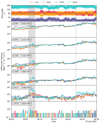 |
Fig. A.1. Differential intensities of energetic electrons measured in all four viewing directions of EPT and HET at the time of shock arrival (gray vertical dashed line). EPT intensities were corrected for ion contamination. This figure is complementary to Fig. 1. |
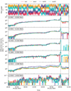 |
Fig. A.2. Differential intensities of energetic electrons measured in all four viewing directions of EPT and HET for the whole event time; the shock arrival is indicated by the gray vertical dashed line. EPT intensities were corrected for ion contamination. This figure is complementary to Fig. 1. |
During shock arrival a steady increase in the differential intensities of the energetic electrons was observed in all four viewing directions of EPT and HET, namely the sun, anti-sun, north, and south. This Letter focuses on the upstream beam observed uniquely by the south telescope. This section provides supportive information for the electrons observed during the event. Complementary to Fig. 1 presented in the main text, Fig. A.1 shows the pitch angle coverage and the same energy channels as observed by all four telescopes. The energy channels are the same as those presented in the bottom panel of Fig. 1.
In Fig. A.1 a number of features related to electron anisotropy at the vicinity of the shock aside from the FABs can also be identified. First, an increase in the intensity of relativistic electrons along PA 180° (second panel from bottom) after the arrival of the shock at 06:22:50 UT. Another is the bi-drectional beams observed at ∼06:18 UT. The identification of such features is possible thanks to the enhanced resolution of the EPD instrumentation.
Figure A.2 presents the full electron event from the solar eruption until the shock arrival at PSP. The same energy channels as in Fig. 1 and Fig. A.1 are shown together with the pitch angles in the top panel for the three day period July 23 – 26, 2022. As in Fig. A.1, a number of observations can be made about the presence of an energetic storm particle event for electrons, which are not the focus of this study. First, the ESP event is seen at all energy ranges presented here, from near-relativistic to relativistic. The second panel from the bottom shows minor increases in the ∼0.5 – 1 MeV electron intensities above the background level. Such relativistic electron observations are extremely rare in IP shocks (Talebpour Sheshvan et al. 2023). Second, the relativistic electrons (the panel above the bottom panel) show a noticeable anisotropy for almost the entire event.
A.1. Ion contamination of Solar Orbiter EPD/EPT measurements
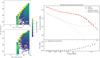 |
Fig. A.3. Ion contamination correction for EPD and EPT channels. The response matrices showing the mean response of all EPT foil channels to H (top left panel) and 4He (bottom left panel) in the corresponding energy channels provided by SIS. (top right panel:) Corrected vs original data of both the electron flux and the background. (bottom right panel:) Ratio of original to corrected flux. |
The Electron Proton Telescope uses the so called magnet-foil technique to separate and measure electrons and ions. This measuring principle has the inherent characteristic that energetic ions will contaminate the electron channels. To determine reliable electron fluxes, the ion contamination in the electron channels must be taken into account. For this work, we used the ion response functions from EPT together with H and 4He flux measurements from SIS-A in order to estimate and correct the ion contamination. In particular, we calculated the count rate of contaminating ions Cion observed in one of the electron channels of EPT by
 (A.1)
(A.1)
where  and
and  are the H and 4He fluxes observed by SIS in the energy channels x and y, ΔEx and ΔEy are the energy widths of the channels x and y, and
  and
and  are the mean responses of EPT for H and 4He in the energy ranges of the channels x and y. Figure A.3 left panel shows the mean response factors
  and
and  for each EPT foil channel in a response matrix.
The ion count rate Cion in each electron channel can be subtracted from the observed count rate in order to obtain an almost clean electron count rate. This electron count rate can be calibrated into electron fluxes using the electron calibration factors from EPT.
Although this method should in principle produce clean electron fluxes, there are some limitations that need to be considered. SIS and EPT have different fields of view, which can lead to over- or undercorrection of EPT electron measurements in the case of anisotropic ion fluxes. Furthermore, the energy coverage and energy resolution of SIS are limited, which also limits the accuracy of the correction. Finally, all ions other than H and 4He are neglected here.
For the time periods investigated here, the anisotropy of the ions was so small, that the assumption of isotropic ion fluxes seemed reasonable for the correction of the ion contamination. Ion species other than H and 4He were not considered here because their flux is generally small compared to H and 4He fluxes and no significant contribution to the observed count rates in EPT is expected.
The correction made based on this method during the investigated period is shown in the right panels of Fig. A.3. The correction is minimal (∼ 1% or lower) up to 100 keV. This ratio increases to > 5% for the energy channels covering > 200 keV energies.
A.2. Ion contamination of Solar Orbiter EPD/HET measurements
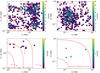 |
Fig. A.4. Pulse height analysis (PHA) of HET electrons. (top left:) PHA data of electrons stopping in detector C, 25 July 2022, 6:00-14:00. (bottom left:) PHA data of electrons stopping in detector C, 25 July 2022, 6:00-6:10. (top right:) PHA data of electrons stopping in detector B, 25 July 2022, 6:00-14:00. (bottom right:) PHA data of electrons stopping in detector B, 25 July 2022, 6:00-6:10. |
The higher energy electron channels of the HET instrument have been found to suffer from proton contamination during strong shock passages. While this issue will be solved in the near future by a software upload from the HET team, careful investigation of the already taken Pulse Height Analysis (PHA) data allows to identify time intervals featuring this contamination. Figure A.4 top left panel shows the PHA data of particles identified by the instrument as electrons penetrating the solid-state detectors A and B of HET, but stopping in scintillator C during a prolonged time interval on 25 July 2022. This representation (energy loss in A+B vs C) allows us to identify several different populations denoted as A) real electrons, which would extend farther to the right for higher energies; B) minimally ionizing particles, that is, protons with energies in the GeV range; and C) lower energy protons. All populations have been reproduced by Monte Carlo simulations. The dashed red lines indicate the energy ranges of the HET electron channel, that is, particles between the right and center red line will be counted in the E5700 channel (the naming scheme refers to Fleth et al. (2023)). Although the data product was crafted such that population B) does not spoil the channel, a strong proton contamination due to track C) can be seen during this day. Figure A.4 bottom left panel shows the same representation, but limited to 6:00-6:10, that is, the time of interest for this study. While the PHA statistic is limited here, it is obvious that the higher electron channels are also heavily contaminated by protons during this time series.Figures A.4 top right and bottom right panels show PHA data of particles identified by the instrument as electrons penetrating detector A, but stopping in detector B (without reaching scintillator C), corresponding to HET’s lowest electron energy channel employed in this study. In contrast to the ABC coincidence discussed above, no clear track as expected from a possible proton contamination is visible in either of the time series. Furthermore, Monte Carlo simulations do not indicate any possibility of proton contamination in this channel.
A.3. Velocity dispersion analysis
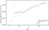 |
Fig. A.5. VDA based on onset times of Solar Orbiter EPT and HET electron channels. The horizontal axis shows the inverse of the average unit-less speed of electrons, as observed in each channel. The vertical axis presents the determined onset time for each energy channel. Onset times observed by EPT (HET) are marked in green (blue). The horizontal error bars represent the width of the energy channels, and the vertical error bars represent the time resolution used to determine the onsets (1 second). The orange line represents the linear fit to the first 16 energy channels of EPT and the first channel of HET, respectively. The onset times that are not considered in the fit have a white middle on the data points. |
Based on the assumption that electrons of all energies were injected at the same time (Vainio et al. 2013), the result of the velocity dispersion analysis (VDA) presents an estimation of the injection time of the energetic electrons and the associated path length from the source to the spacecraft. Figure A.5 shows a well-defined velocity dispersion of the beam in the EPT channels < 300 keV where ion-contamination is low. A good agreement between the EPT channels and the first HET channel is also observed. In this case the estimated path length is ∼13 R⊙, which is 6% of the Sun–Earth distance, making the beam a local phenomenon.
It is worth noting that the VDA could only be performed for the onset times of the first peaks, as it was not possible to obtain reliable starting times for the second peaks that occur co-temporally with the decay of the first ones. A VDA performed on the first peaks themselves also exhibited no velocity dispersion. In this regard, the estimation is approximated to the entirety of the FAB. The onset times were identified using the SEPpy software package (Palmroos et al. 2022), which employs the statistical Poisson-CUSUM method (see, e.g., Huttunen-Heikinmaa et al. 2005) to automatically identify the time of the onset.
Appendix B: The relativistic fast-Fermi model for electron acceleration
The dynamics of particle acceleration in the fast-Fermi model are most effectively described in the de Hoffmann-Teller (HT) frame. In this frame the upstream plasma bulk velocity is parallel to the magnetic field, leading to no upstream motional (−V×B) electric field. The velocity transformation to the HT frame from the normal incidence frame (NIF), a shock rest frame where the upstream plasma flow is directed along the shock normal, is given by
 (B.1)
(B.1)
where  is the shock normal, and V and B denote the upstream bulk velocity and the magnetic field, respectively. The transformation velocity, uHT lies in the shock plane, parallel to the projection of the upstream magnetic field into this plane. The energization of electrons in the upstream solar wind frame arises from transformations to the HT frame, reflection, and then transformation back to the solar wind frame. Denoting the upstream plasma speed in the HT frame by VHT, it was first demonstrated by Sonnerup (1969) that a larger VHT leads to greater energy gain. The relationship between VHT and V can be expressed as
 (B.2)
(B.2)
An electron entering with a parallel velocity v‖ in the upstream plasma frame will reflect upstream with a parallel velocity of −v‖ + 2VHT. In relativistic scenarios, this can be described in terms of momentum p as
 (B.3)
(B.3)
where Γ denotes the Lorentz factor. The associated energy change in the upstream plasma frame is
 (B.4)
(B.4)
Here Γ represents the Lorentz transformation of VHT, defined as  . As indicated in Figure B.1, for θBn approaching 90°, the shock becomes superluminal, making Γ significant. The transformation becomes invalid at θBn = 90°.
The change in particle momentum due to reflection is given by Eq. B.3. To comment on the transformation between the HT and the upstream flow frame, it is possible to use
 (B.5)
(B.5)
 (B.6)
(B.6)
The process of reflection itself happens in the HT frame where the conservation of both the energy and the magnetic moment apply:
 (B.7)
(B.7)
Here p is the momentum and is divided into p∥ and p⊥ corresponding to parallel and perpendicular momentum; eΦHT is the electrostatic potential in the HT and is well known to impact the reflection process (Gedalin & Balikhin 2004).
For relativistic particles we must consider the following form for energy:
 (B.8)
(B.8)
Next, the magnetic moment of the electron can be given as
 (B.9)
(B.9)
This implies that the particle continues to gain perpendicular momentum until a characteristic location at which p∥, HT = 0. This is chosen in such a way that it is implicitly assumed that eΦHT and B are highest in the same region (i.e., the reflection point). An important point to consider here is the value of eΦHT in comparison with the p∥ of the electron. A smaller eΦHT would be insignificant to the incident electron population. This would immediately ensure that the core electrons in any distribution will not be reflected.
It is now possible to make use of the Eq. B.9 and the adiabatic invariance of a relativistic electron in the upstream plasma (−∞) to that of one at the ramp under the influence of the magnetic mirror (Bovershoot):
 (B.10)
Substituting Eq. B.8 in Eq. B.10 one gets
 (B.11)
If we were to work in the frame where  (i.e., the NIF), then there are two electric field components. One is associated with the motion of the plasma Ey, and the other is associated with the shock transition Ex. Transforming into the HT frame then gives
 (B.12)
Using this equation, Goodrich & Scudder (1984) showed that
![Mathematical equation: $$ \begin{aligned} eE_{x , HT} = \nonumber \\ - \frac{\partial }{\partial x} \left[ \frac{m}{2} \left(v^{2}_y + v^{2}_z\right) + m V_{HT} v_z\right] - \frac{1}{n} \frac{\partial p_e}{\partial x} = \nonumber \\ -e \frac{\partial \Phi _{HT}}{\partial x} ,\end{aligned} $$](/articles/aa/full_html/2023/12/aa48120-23/aa48120-23-eq31.gif) (B.13)
(B.13)
where the values of vx and vy are small compared to the upstream electron thermal speed, and so the potential jump ΔΦHT is equal to the change in electron temperature:
 (B.14)
Here Te is in units of eV. The change in electron temperature across the shock usually ranges from tens of eV to about 100 eV (Lembege et al. 2004). Several more proxies can also be used to constrain the electrostatic potential, as done in Hanson et al. (2019) based on the methods established in Gedalin & Balikhin (2004). They are based on ion velocity, ion density, pressure balance, and the electron equation of state. In the case of the shock analyzed here, the potential was found to be between 100 – 200 eV. This estimate is more than a factor of five larger than to the IP shock evaluated by Hanson et al. (2019). The effect of the electrostatic potential is that the acceleration is completely restricted to only the tail of the seed distribution (Leroy & Mangeney 1984).
It is quite clear from this entire ordeal that the most important variable in Eq. B.11 is the mirror ratio Bovershoot/B. In the case of a super-critical quasi-perpendicular shock, the overshoot magnetic field can exceed the simple discontinuity limit (MHD) of 4 (for a gas with adiabatic index 5/3). The reflected electrons therefore form a loss cone distribution which is dependent upon VHT and eΔΦHT. Furthermore, the opening angle α of the so-called “loss-cone” itself is set by the ratio of upstream to downstream magnetic field. The loss-cone angle is such that the resultant distribution is purely made of particles that exceed a certain pitch angle and perpendicular velocity.
Ideally, this may never exceed a certain limit under MHD conservation laws; however, for the considerations made here where the presence of Bovershoot is acknowledged, α = 1/sin(B/Bovershoot). As such, it is evident that the upstream distribution of electrons plays an important role in determining whether the acceleration is significant or not. The “seed” distribution is based upon the in situ spacecraft measurements by Lin (1974), who showed that the electrons have an enhanced supra-thermal tail in the solar wind as opposed to a purely thermal Maxwellian distribution. The supra-thermal tail can be represented by a single kappa distribution that can be defined as
![Mathematical equation: $$ \begin{aligned} f = A \cdot \left[1 + \frac{E}{\kappa E_{\kappa }}\right]^{-\kappa -1} ,\end{aligned} $$](/articles/aa/full_html/2023/12/aa48120-23/aa48120-23-eq33.gif) (B.15)
(B.15)
where A is the normalization constant, and E is the kinetic energy (Maksimovic et al. 1997) in the seed distribution function. For energies where E → Eκ, the distribution behaves as a Maxwellian.
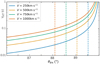 |
Fig. B.1. de Hoffmann-Teller transformation velocity (in units of light speed, c) for different upstream speeds, V (NIF) as a function of θBn. The relationship between these parameters is shown in Eq. B.2. The vertical dashed lines indicate the θBn beyond which the VHT is relativistic. The colors correspond to the different upstream speeds, V. |
The efficiency of acceleration without relativistic effects was originally estimated by Krauss-Varban et al. (1989). Figure B.1 plots Eq. B.2 which shows that as θBn increases above 86°, the HT transformation velocity alone may result in an exponential energy gain of the particle. Therefore, the role of θBn is crucial, as only the electrons that exceed VHT interact with the shock, resulting in a loss-cone distribution. At a certain limit (θBn = 90°) none of the electrons are reflected, and they are transmitted downstream (Ball & Melrose 2001). This aspect of the acceleration mechanism results in the formation of “dilute” beams, that is, beams with very low ratio of beam density to background: nb/n.
Two important issues not discussed here are the “injection” problem and the acceleration timescales. The first issue is fundamental and implies that shock acceleration requires a pre-existing population of supra-thermal particles that can participate in the process. Here it is overcome by the fact that the acceleration mechanism ignores the thermal electrons and only acts on the enhanced tail population of the kappa distribution. The choice of a kappa distribution further simplifies the issue where the supra-thermal tail is enhanced. The reflection timescale for fast-Fermi is dependent upon several factors, the most important of which are the shock strength MA, the thickness of the shock Δx, and Bovershoot. Under the non-relativistic limit for a weak shock with Δx on the order of the ion-inertial length (di = c/ωpi) and for a quasi-perpendicular shock, this can be approximated to depend directly on the ion gyro period (Ωci, Leroy & Mangeney 1984):
![Mathematical equation: $$ \begin{aligned} \tau \sim 4 \Omega _{ci}^{-1} \frac{\Delta x}{M_A} \frac{B_{overshoot}}{\Delta B} \left[1 + \frac{2}{3} \frac{B_{overshoot}}{B}\right] .\end{aligned} $$](/articles/aa/full_html/2023/12/aa48120-23/aa48120-23-eq34.gif) (B.16)
(B.16)
Here ΔB = Boverhsoot − B. The relationship is visualized in Fig. B.2, which shows that for a strong shock with a large magnetic overshoot, its thickness is < di (Hobara et al. 2010). The issue of acceleration timescales becomes important when distinguishing between the various acceleration mechanisms such as fast-Fermi, and first-order Fermi acceleration. The latter, due to its stochastic nature, happens over longer time periods. Meanwhile, the former in the relativistic consideration is on the order of the electron gyro period, and therefore at least two orders of magnitude faster than in the non-relativistic case.
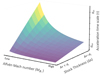 |
Fig. B.2. Acceleration timescale (τ) with respect to shock thickness (Δx) and Alfvèn Mach number (MA). Based on Eq. B.16. Here the color-coding follows a gradient from light to dark, which represents decreasing excursion time (faster acceleration) of the electron. |
A matter of caution in the coordinate transformations considered here is that the reflection process can be treated either purely in the HT frame or the NIF. However, there are frame specific effects such as the transmitted electrons gaining energy in the HT frame due to the potential, while they are unaffected in the NIF due to the convective electric field. If acceleration is purely treated in the HT frame, then the description provided in this section is satisfactory, that is, energy is gained via frame transformation. However, if purely treated in the NIF, the motional electric field ensures that the particles enter a gradient drift motion. In this case, particles will be seen in the direction of the non-coplanar component of the magnetic field.
All Figures
|
Fig. 1. Overview of the in situ shock and energetic electrons observed by Solar Orbiter on 25 July 2022. The arrival of the shock at 06:22:47 is indicated by the vertical gray dashed line in all panels. The first panel shows the differential intensities of energetic electrons observed by the south telescopes of EPT and HET (covering a stable pitch angle of 180° throughout the shown period). The upstream FABs are observed between 06:06:00 and 06:08:30 UT, and are indicated by the gray shaded region. Figure A.1 shows the differential intensities across all viewing directions. The second panel presents the pitch-angle coverage for the different viewing directions of EPT and HET, where the gradients in color indicate the different telescope openings of EPD/EPT (smaller) and EPD/HET (larger). The third and fourth panels show the components of the magnetic field, and bulk flow velocity, while the fifth panel presents the ion number density and proton temperature. |
| In the text | |
|
Fig. 2. Comparison of the peak-intensity electron spectra: observation (top) vs. model (bottom). In the top two panels the points in cyan signify the first peak, while points in blue denote the second peak. The corresponding fits are indicated by orange for the first peak and blue for the second. The background that has been subtracted from each energy channel is represented by points in gray. Top left: Broken power-law fits applied to both peaks. Top right: Broken power-law fits with an exponential roll-over (or cutoff) for the two peaks. Bottom left: Ensemble of runs indicated by the gray shaded region with varying κ ∼ 3 − 4 and θBn ∼ 87° −89.5°. A single power-law fit and exponential roll-over (blue dashed line), and a broken power-law fit (red dashed line) are shown for the modeled mean. The fit for the first peak from top left panel is illustrated by the olive-black dash-dotted line. The mean roll-over (Ec) and break energies (Eb) of the ensemble and its standard deviation are also shown. Bottom right: Modeled results using κ ∼ 3.5 for different θBn (88° −89.5°). The corresponding break energies are indicated by the vertical dashed lines. |
| In the text | |
|
Fig. A.1. Differential intensities of energetic electrons measured in all four viewing directions of EPT and HET at the time of shock arrival (gray vertical dashed line). EPT intensities were corrected for ion contamination. This figure is complementary to Fig. 1. |
| In the text | |
|
Fig. A.2. Differential intensities of energetic electrons measured in all four viewing directions of EPT and HET for the whole event time; the shock arrival is indicated by the gray vertical dashed line. EPT intensities were corrected for ion contamination. This figure is complementary to Fig. 1. |
| In the text | |
|
Fig. A.3. Ion contamination correction for EPD and EPT channels. The response matrices showing the mean response of all EPT foil channels to H (top left panel) and 4He (bottom left panel) in the corresponding energy channels provided by SIS. (top right panel:) Corrected vs original data of both the electron flux and the background. (bottom right panel:) Ratio of original to corrected flux. |
| In the text | |
|
Fig. A.4. Pulse height analysis (PHA) of HET electrons. (top left:) PHA data of electrons stopping in detector C, 25 July 2022, 6:00-14:00. (bottom left:) PHA data of electrons stopping in detector C, 25 July 2022, 6:00-6:10. (top right:) PHA data of electrons stopping in detector B, 25 July 2022, 6:00-14:00. (bottom right:) PHA data of electrons stopping in detector B, 25 July 2022, 6:00-6:10. |
| In the text | |
|
Fig. A.5. VDA based on onset times of Solar Orbiter EPT and HET electron channels. The horizontal axis shows the inverse of the average unit-less speed of electrons, as observed in each channel. The vertical axis presents the determined onset time for each energy channel. Onset times observed by EPT (HET) are marked in green (blue). The horizontal error bars represent the width of the energy channels, and the vertical error bars represent the time resolution used to determine the onsets (1 second). The orange line represents the linear fit to the first 16 energy channels of EPT and the first channel of HET, respectively. The onset times that are not considered in the fit have a white middle on the data points. |
| In the text | |
|
Fig. B.1. de Hoffmann-Teller transformation velocity (in units of light speed, c) for different upstream speeds, V (NIF) as a function of θBn. The relationship between these parameters is shown in Eq. B.2. The vertical dashed lines indicate the θBn beyond which the VHT is relativistic. The colors correspond to the different upstream speeds, V. |
| In the text | |
|
Fig. B.2. Acceleration timescale (τ) with respect to shock thickness (Δx) and Alfvèn Mach number (MA). Based on Eq. B.16. Here the color-coding follows a gradient from light to dark, which represents decreasing excursion time (faster acceleration) of the electron. |
| In the text | |
Current usage metrics show cumulative count of Article Views (full-text article views including HTML views, PDF and ePub downloads, according to the available data) and Abstracts Views on Vision4Press platform.
Data correspond to usage on the plateform after 2015. The current usage metrics is available 48-96 hours after online publication and is updated daily on week days.
Initial download of the metrics may take a while.