| Issue |
A&A
Volume 680, December 2023
|
|
|---|---|---|
| Article Number | A7 | |
| Number of page(s) | 14 | |
| Section | Planets and planetary systems | |
| DOI | https://doi.org/10.1051/0004-6361/202347279 | |
| Published online | 04 December 2023 | |
Phase locking among Saturn radio emissions revealed by Cassini observations
1
Department of Earth and Space Sciences, Southern University of Science and Technology,
1088 Xueyuan Avenue,
518055
Shenzhen, Guangdong, PR China
e-mail: This email address is being protected from spambots. You need JavaScript enabled to view it.
2
LESIA, Observatoire de Paris, Université PSL, CNRS, Sorbonne Université, Université de Paris,
5 place Jules Janssen,
92195
Meudon, France
3
Space Research Institute, Austrian Academy of Sciences,
Graz, Austria
4
Department of Physics and Astronomy, University of Iowa,
Iowa City,
IA,
USA
5
Key Laboratory of Earth and Planetary Physics, Institute of Geology and Geophysics, Chinese Academy of Sciences,
19 Beitucheng western road,
100029
Beijing, PR China
6
Laboratory for Planetary and Atmospheric Physics, STAR Institute, Université de Liège,
Liège, Belgium
7
Laboratory of Optical Astronomy and Solar-Terrestrial Environment, Institute of Space Sciences, School of Space Science and Physics, Shandong University,
264209
Weihai, Shandong, PR China
8
Department of Space Physics, School of Electronic Information, Wuhan University,
430072
Wuhan, PR China
Received:
25
June
2023
Accepted:
2
October
2023
Abstract
Context. Rotational modulation has been observed in different magnetospheric phenomena at Saturn, including radio emissions, which reflect the fundamental plasma processes in key regions. Though previous studies have shown Saturn’s kilometric radiation, 5 kHz narrowband emissions, and auroral hiss to be rotationally modulated, the modulation features of its 20 kHz narrowband emissions are still unknown.
Aims. This work complements previous modulation analysis of Saturn radio emissions by undertaking the analysis of 20 kHz narrowband emissions and comprehensively comparing the phases among the regularly observed radio components.
Methods. We carried out a least-squares analysis using the time series of narrowband emissions, which we derived from an event list based on a previous statistical study on Saturn narrowband emissions.
Results. We reveal a “phase-lock” relation between the 5 and 20 kHz narrowband emissions and Saturn’s kilometric radiation, which suggests these strongly clock-like modulated emissions are connected to the rotating field-aligned current system, with local time preferences for the generation of the radio emissions. This local time preference cannot be well explained by existing theoretical frameworks. Although the phase-lock relation is relatively stable, it may be disrupted during solar wind compression. Therefore, the phase lock between these radio emissions may become a fundamental phenomenon that could help in establishing a global picture of the large-scale dynamics of Saturn’s magnetosphere.
Key words: radiation mechanisms: non-thermal / planets and satellites: gaseous planets / planetary systems
Just to show the usage of the elements in the author field.
© The Authors 2023
 Open Access article, published by EDP Sciences, under the terms of the Creative Commons Attribution License (https://creativecommons.org/licenses/by/4.0), which permits unrestricted use, distribution, and reproduction in any medium, provided the original work is properly cited.
This article is published in open access under the Subscribe to Open model. This email address is being protected from spambots. You need JavaScript enabled to view it. to support open access publication.
1 Introduction
When Saturn’s kilometric radiation (SKR) was first discovered during the approach of Voyager 1 to the planet, the SKR was found to display a rotational modulation near 10 h 39 min 24 ± 7 s (Kaiser et al. 1980; Desch & Kaiser 1981). A slightly modified period was later adopted as Saturn’s rotation period (Davies et al. 1992). Many rotational modulation features at Saturn were subsequently discovered in the decades that followed, including radio emissions (Gurnett et al. 2009a,b; Ye et al. 2016; Fischer et al. 2015), magnetic field perturbations (Espinosa & Dougherty 2000; Andrews et al. 2008; Provan et al. 2009), energetic neutral atoms (Carbary et al. 2008a; Paranicas et al. 2005), the plasma sheet (Carbary et al. 2008b), auroral features (Nichols et al. 2008), and even the location of the magnetopause and bow shock (Clarke et al. 2010, 2006). Moreover, the modulation in the northern and southern hemispheres were found to show two distinct periods (~10.6 h and ~10.8 h) from 2004 until 2009 (Gurnett et al. 2009b, 2010). Interestingly, these two periods in the northern and southern hemispheres derived using the SKR data were then found to show seasonal variations, with the modulation rates in the two hemispheres converging near equinox (11 August 2009; Ye et al. 2016; Fischer et al. 2015; Gurnett et al. 2010; Andrews et al. 2012) and showing a complicated behavior after the equinox. Only in the last three years of the Voyager mission were the two SKR periods again clearly separated, with the northern period, ~10.8 h, being longer than the southern period, ~10.7 h (Ye et al. 2018).
Interpretation of the SKR rotational modulation has evolved over time. Initially, during the Voyager era, it was described as a strobe-like or clock-like feature occurring on the dawn local time sector (Warwick et al. 1981). Subsequent research using Cassini measurements revealed a more complex behavior, indicating that SKR is modulated as a rotating beam, akin to a searching light co-rotating with the planet but also exhibiting strong strobelike modulation in the morning local time sector (Lamy et al. 2009; Lamy 2011; Andrews et al. 2010; Provan et al. 2014). The high frequency limit of SKR has also suggested a combination of a strobe-like and rotating beam modulation (Wu et al. 2023). Studies have found that the periods of magnetic field oscillation in the northern and southern hemispheres of Saturn are consistent with the modulations observed in the northern and southern SKR data (Andrews et al. 2008, 2010, 2012). Additionally, a combination of both northern and southern modulation periods in the magnetic field data has been observed at the equatorial magnetosphere (Provan et al. 2011). These magnetic field perturbations display quasi-uniform characteristics in the equatorial region and quasi-dipolar patterns at high latitudes, indicating the presence of two independent high-latitude auroral field-aligned current (FAC) systems co-rotating with the planet at the northern and southern SKR periods (Andrews et al. 2010, 2019; Provan et al. 2014). These current systems, initially proposed by Andrews et al. (2010), have been observed multiple times by Cassini (Hunt et al. 2014, 2015; Bradley et al. 2018) and are now referred to as planetary period oscillation (PPO) current systems. The subsequent studies that followed these earlier investigations are generally now referred to as PPO studies.
As SKR emissions have been demonstrated to originate along auroral magnetic field lines with electron precipitation, that is, the upward field-aligned currents (Lamy et al. 2009, 2018), these PPO current systems identified by Andrews et al. (2010) have provided a reasonable explanation for the sources of SKR emissions and their modulation features. The rotating beam modulation of SKR can be naturally attributed to the rotation of these two current systems. Furthermore, the pronounced dawnside strobe-like SKR modulation can be explained by the interplay of the PPO current systems and potential quasi-steady upward currents on the morningside resulting from solar wind interaction (Southwood & Kivelson 2009; Cowley et al. 2004). More recent works have further confirmed the seasonal variations of the magnetic PPO periods that are mostly identical to the SKR modulation periods, except during 2013 (Provan et al. 2013, 2014, 2016; Cowley & Provan 2013). Detailed examinations of PPO current densities have revealed an overall similarity between the summer and winter hemispheres, suggesting a more intricate coupling process with Saturn’s seasons (Bradley et al. 2018; Cowley et al. 2020).
Rotational modulation analysis of Saturnian radio emissions, including the auroral hiss (Gurnett et al. 2009b), SKR (Fischer et al. 2015; Gurnett et al. 2010; Lamy 2011; Ye et al. 2016, 2018; Provan et al. 2014, 2016), and the 5 kHz narrowband (NB) emissions (Ye et al. 2016, 2010a; Wang et al. 2010), has revealed similar modulation features and helped in further understanding their generation mechanisms. Auroral hiss has been proven to be modulated like a rotating beam because its low-frequency whistler-mode mostly propagates along the source field lines that co-rotate with the planet (Gurnett et al. 2009a). The 5 kHz NB emissions are modulated like a clock (strobe-like), which means their sources are like a light fixed in a local time blinking on and off.
The NB emissions were discovered by the Voyager spacecraft and are referred to as 5 kHz NB and 20 kHz NB according to their frequencies (Wang et al. 2010; Gurnett et al. 1981; Ye et al. 2009; Wu et al. 2021). Both the 5 kHz and 20 kHz NBs can be produced via a mode conversion process from the Z mode to the L-O mode (Ye et al. 2009, 2010b; Menietti et al. 2019), as previously observed and discussed in the studies of the terrestrial ionosphere (Eckersley 1933; Ellis 1956; LaBelle & Treumann 2002; Benson et al. 2006). The 20 kHz NB can also be mode converted from the upper hybrid resonance (UHR), which turns into the Z mode at density gradients, and then the Z mode can mode converted to the L-O mode (Ye et al. 2009). The Z-mode emissions (at both 5 kHz and 20 kHz) can be excited via plasma distributions with temperature anisotropies and a weak loss cone, as observed in the NB emission source regions (Menietti et al. 2019, 2011). However, there is no unambiguous observation of the Z-mode emissions in the source region with enough electron pitch-angle coverage, leaving the details of the generation mechanism unresolved. The NB emissions are believed to be generated in the interior of the Enceladus plasma torus. Blocked by the plasma torus, the 20 kHz NB emissions only propagate to high latitudes and are rarely observed at low latitudes outside the plasma torus, whereas the 5 kHz NB emissions can be reflected to this region by the magnetosheath (Wu et al. 2022, 2021).
The rotational modulation of the 5 kHz NB emissions has been analyzed previously (Ye et al. 2010a, 2016). The dual periods of the 5 kHz NB emissions have been observed in each hemisphere, which is in contrast to the case of the SKR, where one period occurs in each hemisphere (i.e., north–south asymmetry). The L-O mode 5 kHz NB emissions are mode converted from Z-mode emissions, which may cross over to the other hemisphere before mode conversion to the L-O mode (Ye et al. 2010b). The detailed propagation features of the Z-mode NB emissions for both the 5 and 20 kHz NB emissions are still unknown and will be investigated in an isolated ray-tracing study. Such an investigation may indicate that the propagation is similar to that in the Earth’s plasma environment, where it has been shown that the Z-mode waves can propagate within field-aligned electron-density irregularities (FAls) with little attenuation (Calvert 1995; Carpenter et al. 2002; Reinisch et al. 2001). Therefore, the dual periods of 5 kHz NB emissions could be attributed to Z-mode NB emissions generated in different hemispheres propagating and crossing to the other hemispheres.
In this work, we analyze the modulation of the 20 kHz NB emissions and compare the phase relations between the SKR, the 5 kHz NB emissions, and the 20 kHz NB emissions. The modulation characteristics of the 20 kHz NB are similar to those of the 5 kHz NB emissions that are strongly clock-like modulated, display dual modulation periods, and have seasonal variations in the modulation rates. The comparisons of different radio components suggest the emissions are always observed in a particular sequence, which implies that the magnetospheric processes that cause the excitation of the radio emissions occur in a temporally or spatially organized sequence.
2 Data and methodology
We used the wave electric field data measured by the Radio and Plasma Wave Science (RPWS) instrument (Gurnett et al. 2004) on board the Cassini spacecraft. The RPWS wave electric field data are from the LESIA/Kronos collection with n2 level data (Cecconi et al. 2017a) and the wave polarization data with n3d data (Cecconi et al. 2017b). We note that the n3d data give the wave polarization information, which is derived by assuming the waves originated from the center of Saturn (Cecconi & Zarka 2005). From Day 183, 2004, to Day 258, 2017, the SKR intensity was obtained by integrating the electric field spectral power in the frequency range from 80 kHz to 500 kHz and separated into the northern and southern hemispheres according to the spacecraft latitude and circular polarization. The circular polarization threshold was used to distinguish the SKR emission that was either generated at the northern hemisphere (circular polarization <−0.5) or the southern hemisphere (circular polarization >0.5). The derived SKR intensities in the two hemispheres were normalized by the mean value of the intensities within one Saturn rotation (in this study, 10.6 h) to eliminate the radial distance effect. For the period after 1 December 2016, the SKR power was separated only by latitude (10° used in this work) due to uncertainty in the polarization measurement of SKR when Cassini was close to Saturn (the assumption of Saturn’s center as the source of SKR was not good anymore). The procedure to derive the SKR power time series is the same as in Ye et al. (2018). The Saturn Longitude System 5 (SLS5) longitude system used in this work to produce Fig. A.1 is from Ye et al. (2018).
The low-frequency extension of SKR into the frequency range of the NB emissions contaminates the integrated time series of the NB emissions from time to time (Reed et al. 2018). Hence, instead of integrating the spectral power in the frequency ranges of NB emissions directly, the time series of the 5 kHz NB and 20 kHz NB are obtained by using the event list derived by computer selection and aided by human confirmation (Wu et al. 2021). During the whole Cassini-Saturn orbital tour (from Day 183, 2004, to Day 258, 2017), the start and end times of the NB emissions were obtained when the intensity and circular polarization exceeded certain preset thresholds of 23 dB and |υ| > 0.3, respectively. When there was an NB emission present, the intensity was assigned a value of one, and in intervals of no NB, the value assigned was zero. In this way the contamination with SKR was eliminated. The modulation analysis of the zero-one time series has previously been applied successfully to the auroral hiss (Gurnett et al. 2009b). Finally, we obtained four catalogs for the 5 kHz NB, 20 kHz NB, northern hemisphere SKR, and southern hemisphere SKR. For each series, the data values are organized at a 10-min cadence.
We used the least-squares spectral analysis (LSSA) method (Scargle 1982) to derive the rotational modulation spectrogram of the radio emissions. The parameters used in the analysis are the same as the previous studies (Gurnett et al. 2009a,b, 2010; Ye et al. 2016, 2018) and are detailed below.
To calculate the modulation spectrogram, we first truncated the original integrated wave power time series into a series of 240-day sequences with an overlap of 210 days (The 240-day time window was shifted forward in 30-day steps). The power time series was then weighted by a Hanning window of the same length. The length of 240 days (540 Saturn rotations) guarantees a resolution of 1.5° per day near Saturn’s rotation period, as suggested by previous studies (Gurnett et al. 2009b; Ye et al. 2016, 2018). The 240-day time series were then sorted and averaged to the longitude of the sun (clock-like source),

and the longitude of the spacecraft (rotating beam source)

in one-degree bins by assuming a series of rotation rates (from 785° to 830° around Saturn’s rotation rates). For each rotation rate ω0, a sinusoidal curve was fitted to the data to get the amplitude (A) and phase (ϕ). Therefore, the best-fit parameters would have the strongest modulated power (defined as P = (2A)2) and correspond to the best rotation rate ω0. After each modulation power analysis, the 240-day window was advanced by a time step of 30 days. We note that in the calculation result of one 240-day window, there could be several power peaks. The modulation rates should not be decided only by using the maximum power peak but should be decided by combining the information in the modulation spectrograms as discussed in Sect. 5.
3 Clock-like modulated narrowband emissions
The previous studies (Ye et al. 2016, Ye et al. 2010a; Wang et al. 2010) reported that the 5 kHz NB emissions are modulated with a clock-like source. To explore whether the 20 kHz NB are modulated like a clock or a rotating beam, we reorganized the time series of NB emissions as a function of longitude of the Sun (clock-like source) and longitude of the spacecraft (rotating-beam source). (The NB time series were obtained from the event list given by a former study (Wu et al. 2021) detailed in method section.) The reorganized series were then fitted by a sinusoidal function (with amplitude A; period 2π / ω0, ω0 is the assumed modulation rate; and phase ϕ) to get the fitted power (where P is defined as P = (2A)2). These fitted powers are plotted in panels a and b of Fig. 1 to show which modulation rates are fitted better. A stronger power means the series is organized better by the assumed modulation rate. This fitting algorithm is often referred as LSSA.
Figure 1 shows the calculated LSSA result of the NB emissions’ time series with a 240-day window from 5 November 2008 to 3 July 2009. During this interval, Cassini made 21 high inclination orbits with peak latitudes exceeding 50°. The modulation power P is plotted versus the assumed rotation rate ω0. As shown in panels a and b, the blue lines (assuming a rotating beam source) show much weaker modulation power relative to the red lines (assuming a clock-like source), suggesting that the time series reorganized by a beam source cannot be fitted better than the series reorganized by a clock-like source. We note that this test requires a relatively large local time coverage of the spacecraft orbits in order to distinguish the two types of modulation from each other, and it does not completely exclude the other.
During the calculation time interval, the orbits of Cassini do span the whole local time range. To be more rigorous here, we concluded that both the 5 kHz and 20 kHz NB are modulated more like a clock than a rotating beam. The two rotation periods near 801.3° and 814.1° per day are consistent with results of previous works (Ye et al. 2018) and similar to the periods of the SKR modulation during this time interval, as indicated by the vertical black dashed lines in both panels of Fig. 1.
4 Dual periodicities of narrowband emissions in both hemispheres
The two modulation periods (~10.6 h and ~10.8 h) corresponding to the two hemispheres were revealed by the analysis of the northern hemisphere SKR and southern hemisphere SKR (Gurnett et al. 2009a). The dual modulation periods observed in one hemisphere of the 5 kHz NB emissions are explained by the emissions crossing hemispheres before being observed by Cassini, as reported in the earlier study (Ye et al. 2010a). The 20 kHz NB emissions are mainly observed at high latitudes, and almost never observed within 10° latitude of the equator (Wang et al. 2010; Wu et al. 2021). Therefore, to test the north-south asymmetry of the modulation of the 20 kHz NB, we carried out the LSSA by separating the 20 kHz NB series according to the observer’s latitudes: Lat >10° for northern hemisphere and Lat <−10° for southern hemisphere. For both hemispheres, the LSSA was made assuming a clock-like modulation, as confirmed in the previous section. As shown in panel a of Fig. 2, the modulation rates in the northern hemisphere show dual periods similar to the earlier results for the 5 kHz NB (Ye et al. 2010a). The dual modulation rates suggest that the 20 kHz Z-mode NB could also cross the hemisphere before mode conversion to the L-O mode because the 20 kHz L-O mode NB cannot cross the hemisphere due to being blocked by the plasma torus, which is generated by the cryovolcanic activities of Enceladus at Saturn (Wu et al. 2021; Persoon et al. 2020). The propagation characteristics of the Z-mode NB emissions are not well studied at present and will be covered in future studies.
A total of 372 cases of 20 kHz NB were observed during the 240-day interval from 5 August 2008 to 3 July 2009 (interval of Fig. 2). This interval was chosen due to the clear dual periodicity including 249 cases in the northern hemisphere and 123 cases in the southern hemisphere. Therefore, the modulation spectrum for the southern hemisphere in panel b of Fig. 2 does not show two clear peaks at the SKR periods due to fewer cases of 20 kHz NB being observed in the southern hemisphere. It is also possible that during this time interval, the southern PPO modulation dominates over the northern PPO (Provan et al. 2016), which makes it difficult to distinguish the weak northern modulation features from the data.
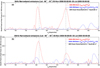 |
Fig. 1 Clock-like modulation of NB emissions. Panel a: clock or rotating beam test for 5 kHz NB. The horizontal axis of ω0 encompasses the assumed modulation rates of 785 to 830° per day, which was chosen to be near the rotation rate of Saturn (10.7 hours = 807° per day). The vertical axis is the fitted peak-to-peak modulation power giving the fitted peak power of the 240-day time series under the assumption of each ω0. The two solid lines show the modulation rates of 5 kHz NB emissions under the assumption of a clock-like source (red) and a rotating beam source (blue). Panel b: similar format as panel a but for 20 kHz NB emissions. The black dashed lines mark the modulation rate in the same 240-day window derived from the SKR intensities. The 5 kHz and 20 kHz NB time series used in this window are not separated into two hemispheres according to latitude. |
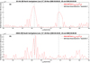 |
Fig. 2 North-south asymmetry test of the 20 kHz NB emissions. Panel a: modulation rate of the 20 kHz NB emissions in the northern hemisphere, similar to Fig. 1. Panel b: similar format as panel a but for the southern hemisphere. The 20 kHz NB time series used in this window is separated into two hemispheres according to the latitudes (Lat: >10° and < −10°). |
5 Seasonal variations of the rotational modulations of Saturn radio emissions
In Fig. 3, the LSSA derived modulation power P is plotted as a function of the modulation rate and time. These spectrograms were produced by reproducing the modulation rates in Fig. 1 but with different time intervals for the time series, as detailed in the method section. Figures 3a–c are the reproductions of Fig. 1 of Ye et al. (2018) and Fig. 4 of Ye et al. (2010a). The previous work showed the two SKR modulation periods to have seasonal variations according to the season at Saturn (Lamy 2011; Gurnett et al. 2010; Ye et al. 2016; Provan et al. 2014, 2016; Andrews et al. 2019). Near Saturn’s equinox in August of 2009, when the northern hemisphere of Saturn transitions from winter to spring (illustrated in panels a and b of Fig. 3), the SKR modulation rates in the two hemispheres (indicated by the white lines) tend to converge near the equinox. We show the modulation periods of 5 and 20 kHz NB in panels c and d of Fig. 3. The green and orange lines overplotted in panels c and d mark the SKR modulation periods in the northern and southern hemispheres from panels a and b, respectively; these two lines correspond to the results of Ye et al. (2018). Overall, one can see that the modulation power of the 5 and 20 kHz NB emissions in panels c and d align with the SKR periods and converge near the end of 2009. The 20 kHz NB emissions only occur in regions with latitudes larger than 10°, and they have a high occurrence probability only above 30° in latitude (Wu et al. 2021). Therefore, the modulation signal only shows up during high inclination orbits, as shown in panel e. Despite the high inclinations, there are practically no signals for the year 2014 nor for the last year of the mission in 2016–2017. For the latter period, this is mainly due to the short duration Cassini spent at latitudes above 30°, which was just about one day for each hemisphere and orbit during the F-ring orbits and only about half a day for each hemisphere and orbit for the proximal orbits. Cassini also spent just a short time at high southern latitudes during 2014 but typically around 3 weeks per orbit at northern latitudes above 30° in 2014. In that case, the absence of the modulation signal could be a combination of Cassini’s large distance and local time. Cassini was mostly between 3 and 9 h LT (where NB emissions are less common) and at distances beyond 35 Saturn radii, where the detected power is small and might have partly fallen below the intensity threshold. (The threshold used to distinguish the 20 kHz NB is detailed in the Method Section.) The PPO periods derived from the magnetic field measurements (Andrews et al. 2010; Provan et al. 2013, 2016, 2019) are also overplotted as blue and pink lines in panels c and d in order to compare the modulation periods of NB emissions and the PPO periods. The overall modulation periods of SKR, PPO, and the NB emissions are consistent with each other, with the possible exception of the second modulation signal of the 20 kHz NB at the beginning of 2013, as shown in panel d, which seems to be about 5 deg per day slower than the other southern periods derived from the 5 kHz NB, the SKR, and the magnetic field data.
6 Phase lock of Saturn radio emissions
The phase relation between the SKR and the 5 kHz NB was previously reported to be around 90° in both the northern and southern hemispheres (from early 2008 to late 2009), suggesting that SKR could lead the 5 kHz NB by 2–3 h (90°/360°*10.6 h = 2−3 h, 1 Saturn rotation = 10.6 h; Ye et al. 2018). The phase relations between different radio emissions can be obtained by comparing the ϕ parameters fitted by the sinusoidal function in the LSSA algorithm. To determine the phase relation between the SKR, 5 kHz NB, and 20 kHz NB, we choose the time intervals when the modulation power for all three emissions was strong, from November 2008 to September 2009, as can be seen in Fig. 3. During this time interval, the southern hemisphere SKR modulation is weak, but the phase difference still gives stable values.
In Fig. 4, the pink squares and the black points represent the phase difference for the northern and southern hemispheres. The leading angle between SKR and the 5 kHz NB is around 120° in the present work (129.7° ± 26.6° in the north and 122.4° ± 26.6° in the south), as shown in panel a of Fig. 4. This difference, compared to the previous work, could be due to the 5 kHz NB data (zero-one series, see the method section) we used in this work, which is different from the integrated intensities used in the earlier work (Ye et al. 2010a). The phase relation shows that the SKR leads the 5 kHz NB by around 120° (panel a), and it leads the 20 kHz NB by around 180° (panel c), which means that the SKR, 5 kHz NB, and 20 kHz NB are observed sequentially according to the phase relation. The relative phase angles between these three radio emissions were relatively stable during the ten months between November 2008 and September 2009. The point scatter in Fig. 4 is mostly distributed within a 50-angle range with few exceptions. The phase differences in the two hemispheres show a consistent variation, which implies that the relative phase relations in the two hemispheres might follow the same triggering sequence, even though the modulation periods are different in the two hemispheres. The phase differences in panel b between the 5 and 20 kHz NBs are 55.3° in the north and 107.2° in the south, and the latter is due to the outlier in the phases of the southern 20 kHz NB on 4 January 2009 caused by the weak modulation of the 20 kHz NB, as shown in panel d of Fig. 3. The time lag between the observations of different components could be estimated using the phase differences. For SKR and 5 kHz NB, this is 120°/360° × 10.6 h ≅3–4 h, and for SKR and 20 kHz NB, it is 180°/360° × 10.6 h ≅5–6 h (1 Saturn rotation is roughly 10.6 h).
For the first time, we report that these three radio emissions show this kind of “phase-lock” relation (the relative phase relations remain the same) during these 10 months, which suggests that the underlying magnetospheric physical processes triggering these three radio emissions might be very similar or interrelated. The phase lock can also be roughly identified in the electric field spectrogram, as given in Fig. 5. The wave electric field spectrogram in panel a shows a roughly three-day observation of Cassini RPWS. This observation was selected during the time interval of Fig. 4 to give an intuitive illustration of the phase lock. The phase lock can be approximately identified from the occurrence order as indicated by the arrows in different colors in panel a. We plotted the intensities at the frequencies of 71.2 kHz, 15 kHz, and 5.1 kHz to give a more straightforward picture in panels b–d. The three horizontal white lines in panel a mark these three frequencies representing the intensity variations of SKR, 20 kHz NB, and 5 kHz NB. We ordered the sequence of the phase relation in panels b–d. As indicated by the oblique red dashed lines, a phase-lock relation can be observed. We note here that these lines are different from the LSSA input time series that were integrated over a large frequency range or the zero-one time series (detailed in method section), and they were only adopted to show the rough occurrence order. The detailed time lags for these cases are not easy to identify directly from the time series in panels b–d of Fig. 5, as the peak locations are not the averaged ones but for the specific frequencies. The phase angle varies over a small range, as indicated by the slight wobbling of the oblique red lines. The overall phase relation is stable in the three-day observation interval and consistent with Fig. 4 and supports a phase-lock relation.
Due to a lack of stable observations of the SKR, 5 kHz NB, and 20 kHz NB emissions, the phase relationship at other time intervals cannot be determined from the LSSA method. However, the SKR modulation power is much stronger than the NB emissions, and there exists the longitude systems derived from the SKR intensity modulation, such as the SLS5 (Ye et al. 2018). The zero degree of the sub-solar longitude in the SLS5 corresponds to the maxima of SKR intensity (Ye et al. 2018). Therefore, the phase relation of these three radio components from the LSSA results should be the same if we organized the time series (occurrence longitude) of the NB emissions in the SLS5 systems. The results are given in Fig. A.1, and they sug gest that the phase relation between the SKR and the 5 kHz NB is consistent with the LSSA results in Fig. 4, and it is likely to be stable during the whole Cassini mission, whereas the features of the 20 kHz NB emissions are not very obvious due to the lack of observations.
We note here that this phase relation can sometimes change temporarily, as indicated in Fig. A.2, and that the occurrence sequence of the “phase-locked” radio components changed. We refer to this phenomenon as the “disturbed phase lock”, or “loss of phase lock”. These disturbed phase locks are usually observed near the sudden enhancements of the SKR, which could be related to strong magnetospheric dynamics, such as the solar wind compression-induced hot plasma injection (Jackman et al. 2009, 2010; Reed et al. 2018; Bunce et al. 2005). A disturbed phase lock observed during the compression of the solar wind in a previous study suggests this could be attributed to the external influence on the magnetosphere (as indicated in Fig. 2 of Jackman et al. 2009). In fact, a statistical study of the “low-frequency extension” of SKR in a previous work (Reed et al. 2018) has shown that the timing of the solar wind-related SKR is poorly organized by the Saturnian longitude system that is derived from the rotational modulation of the SKR, which implies the occurrence sequence of the radio emissions can be influenced by the external driver.
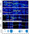 |
Fig. 3 Least-squares spectral analysis spectrograms of Saturn radio emissions from 2004 to 2018. The color-coded spectrograms show the modulation power as a function of universal time in the horizontal axis and the modulation rate in the vertical axis. Panels a–d respectively show the results for the northern hemisphere SKR, the southern hemisphere SKR, the 5 kHz NB emissions (in both hemispheres), and the 20 kHz NB emissions (in both hemispheres). Panel e shows the Cassini latitudes during its Saturn orbital journey. The green and orange lines are the northern and southern SKR periods as derived by Ye et al. (2018). The blue and pink lines are the northern and southern PPO periods as derived by Provan et al. (2013, 2016, 2019). |
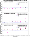 |
Fig. 4 Clock-phase difference of Saturn radio emissions. Panel a: relative phase between SKR and 5 kHz NB emissions in the northern (black) and southern (pink) hemispheres. Panel b: relative phase between 5 kHz NB emissions and 20 kHz NB emissions. Panel c: relative phase between SKR and 20 kHz NB emissions. |
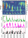 |
Fig. 5 Relative phase of the Saturn radio emissions. Panel a: Cassini RPWS wave electric field spectrogram. The horizontal white dashed lines mark the frequencies of 71.2 kHz (corresponding to SKR), 15 kHz (corresponding to 20 kHz NB), and 5.1 kHz (corresponding to 5 kHz NB), which are used in the following panels to plot the frequency intensity versus time variation. The blue, pink, and black arrows in panel a indicate the three radio emissions. Panels b–d: spectral density in units of dB above the background. The oblique red dashed lines depict the rough phase relation between the three radio emissions. The peaks marked by the oblique red dashed lines correspond to the blue, pink, and black arrows in panel a, which correspond to the main emissions of SKR, 5 kHz NB, and 20 kHz NB. The black shaded regions in panels b–d indicate the regions that are polluted by the low-frequency extensions of SKR. The relatively constant relations shown suggest a phase-lock situation. |
7 Discussion and conclusions
Many models have been proposed in order to explain the rotational modulation phenomena observed at Saturn since their discovery. The drivers of the modulation have been proposed to be either in the thermosphere (e.g., the vortical flow of the zonal wind; Smith 2011; Jia et al. 2012); ionosphere (e.g., the variation in Pederson conductivity; Gurnett et al. 2009a, 2010); or magnetosphere (e.g., the mass ejection of Enceladus, the interaction with Titan, and the oscillations of the plasma; Southwood & Cowley 2014; Goldreich & Farmer 2007; Khurana et al. 2009; Burch et al. 2008; Winglee et al. 2013). All these models require the formation of large-scale FAC systems to account for the modulation features observed in several studies (Hunt et al. 2014, 2015). The PPO current systems can be an ideal candidate to describe these phenomena (Andrews et al. 2010, 2019; Southwood & Cowley 2014; Cowley & Provan 2017; Provan et al. 2018). The simulation work of Jia et al. (2012) successfully reproduced many modulation features observed at Saturn by introducing the twin-cell vortices within the atmosphere of Saturn’s northern and southern polar regions, which drive the FACs. The phase lock has the potential to serve as a valuable observation feature for remote monitoring of the large-scale magnetospheric convection pattern.
The phase lock could be explained in the context of the generation mechanisms of the radio components and in combination with the PPO current systems. The SKR has been shown to be related to the upward FAC in the PPO current system, which is connected to the partial ring current (Provan et al. 2009). The FAC intensities observed in the northern hemisphere are well modulated by the modulation period of the magnetic field and are possibly related to the generation of SKR (Hunt et al. 2015). The rotation of the FAC system directly gives rise to the modulation of SKR, especially in conjunction with its passage through the morning sector (Andrews et al. 2010; Provan et al. 2014; Southwood & Cowley 2014; Southwood & Kivelson 2009). The temporal and spatial variations of the SKR-FAC may be further coupled to the reconnection-driven electron precipitation processes.
The 5 kHz NB emissions are possibly generated at the inner edge of the plasma torus and the high-latitude region close to the SKR source region. Wing et al. (2020) found that the 5 kHz NB is well correlated with the so-called type-2 injection (Mitchell et al. 2015), which is related to flux-tube interchange in the inner magnetosphere (Hill 1976; Wing et al. 2022). The interchange injections also build up the FACs and further transport the particles, as shown by the study of Radioti et al. (2019). The injections may lead to the intensifications of the PPO FACs, and the injection-produced FACs may be further coupled to the PPO current systems that drive by the twin-cell vortices in the atmosphere (Andrews et al. 2012, 2019; Hunt et al. 2015; Cowley & Provan 2017). The source plasma for the 20 kHz NB could be transported in a similar way as for the 5 kHz NB, but to different source locations due to the differences in wave frequencies.
The explanation of the phase-lock or the occurrence sequence can then be simplified into two scenarios: (1) the spatial effect, where all the emissions are produced by rotating upward FACs, and the phase lock is generated due to the visibility effect from the radio source regions rotating together with the FACs into the field of view of the spacecraft one-by-one, and the (2) temporal effect, where the emissions prefer to be generated at different locations and are excited sequentially following the phase-lock sequence as the FACs rotate through different LTs (local times) and transport the source plasma to the radio source regions.
For spatial effect scenario, the FACs’ systems at the polar region usually consist of the upward and downward currents, as shown in the magnetic field measurements (Provan et al. 2018; Bradley et al. 2018; Andrews et al. 2010) and the simulations (Jia et al. 2012). The two upward FACs, which transport the electrons to the planet side are located on the two sides of the planet and show asymmetries in location and intensity, for instance, Fig. 1 of Provan et al. (2018) and Fig. 2 of Jia et al. (2012). It is possible that SKR is produced via the upward FACs on one side of the planet, and NB emissions are produced via the upward FACs on the other side. We note that the upward FACs causing the NB emissions would be located at lower L shells (compared to the upward FACs of SKR). Hence, they could produce NB emissions within 5 Rs (Saturn Radii), where the 5 and 20 kHz NB emissions were found to be most intense (Wu et al. 2021). Strong FACs were not only found at 15–20 Rs (where they might cause SKR) but also closer to the planet. This is evidenced in Fig. 12 of Andrews et al. (2019), in which the north-south current density is plotted in Saturn’s equatorial plane. Then the phase lock could be generated simply by the rotation of the current systems as the favorable side of the upward FACs rotates into the field of view of Cassini. This also implies no isotropic propagation, but an angularly limited beaming of the NB emissions.
For the temporal effect scenario, the phase lock suggests that the source regions of different radio components are activated one after another as the FACs rotate and transport the hot plasma to the source regions where the plasma environment favors the excitation of the radio emissions, such as the well-known morningside peak of SKR (Lamy et al. 2009) is followed by the 5 kHz NB and the 20 kHz NB. The NB emissions tend to be more frequently observed on the duskside (Wang et al. 2010; Wu et al. 2021), corresponding to the FACs rotating from the morningside to the duskside.
Numerous studies have indicated that the rotating beam modulation of SKR comes from the rotation of the PPO current systems, while the strong morningside clock-like modulation of SKR comes from the PPO current systems’ interaction with the localized upward currents (Provan et al. 2014, 2019; Andrews et al. 2019; Southwood & Kivelson 2009), hence a combination of scenario 1 and scenario 2. This could also be true for the NB emissions because the visibilities of NB generally cover all LTs, and the 5 kHz NB tends to be more frequently observed from a spacecraft on the duskside (Wang et al. 2010; Wu et al. 2021). Therefore, the phase lock of the radio emissions is possibly produced by the rotating FAC system and an LT preference for the generation of the emissions when the FACs rotate to a certain LT range. In principle, there are two different rotating PPO FAC systems: one in the northern hemisphere and one in the southern hemisphere, as reported by numerous studies (Provan et al. 2021; Andrews et al. 2010; Hunt et al. 2014, 2015). Hence, for both scenarios, it is possible to have two different rotation periods at the same time.
The phase differences or time lags can be used to estimate either the angular distance of the FACs for the different radio components (scenario 1) or the LT distribution of the radio sources (scenario 2). For example, the ~120° phase difference between the SKR and 5 kHz NB would correspond to ~120° angle distances between the SKR FACs and the NB FACs, or a ~3–4 h time lag between the SKR source LT and the NB source LT. The calculation of NB modulation suggests the clock-like sources are dominant (scenario 2), and the co-rotation sources are weaker (scenario 1) if compared to the clock-like sources.
The discussions above are based on the view from the FACs, which could be driven by the vortices in the ionosphere or be formed due to magnetospheric phenomena, such as reconnection and interchange instabilities, or in a more complicated picture, these phenomena could all be coupled together. That is, the injections and/or interchange instabilities could have a local time preference (Azari et al. 2019), the convection of the hot plasma to the source region of radio emissions could take time, and the process of which is controlled by the PPO current system in each hemisphere is further influenced or controlled by the twin-cell vortices in the atmosphere. The detailed plasma transportation processes, for example, how these FACs are formed, how they transport the hot plasma, and how these processes generate the phase lock, are still unknown and are left to be explored in future studies.
The relatively stable phase relation implies that this possible plasma circulation process is similar to an intrinsic mode of the whole magnetosphere. Hence, it suggests a regular large-scale magnetospheric convection pattern. The occasionally observed “disturbed phase lock” near the enhanced SKR suggests the occurrence sequence could be temporarily changed due to an external driver, such as the solar wind compression. Based on these characteristics, we suggest that the occurrence sequence of the radio emissions could be a good monitor to probe the plasma circulation within the Saturnian magnetosphere.
To summarize, we analyzed the modulation of Saturn radio emissions and compared the phase relationship between different components. This work for the first time derived the rotational modulation characteristics of the 20 kHz NB emissions at Saturn, and it showed similar modulation features as those of the 5 kHz NB. In particular, the dual modulation rates observed in one hemisphere could be explained by the Z-mode waves crossing the hemisphere. The excitations of the radio emissions are possibly related to the FACs, which could be driven by the twin-vortex in the upper atmosphere or be formed via reconnection and interchange processes co-rotating with the planet. The phase-lock relation between different radio components, which probably reflect an LT preference in the plasma processes that generate these emissions, could provide crucial constraints that would aid in the understanding of the global magnetospheric picture and the current circuit system.
Acknowledgements
This work was supported by the Strategic Priority Research Program of the Chinese Academy of Sciences (grant no. XDB 41000000). S.Y. and S.W. thank the support of NSFC projects 42274221 and 42074180. We thank the support of Science, Technology and Innovation Commission of Shenzhen Municipality program (STIC20200925153725002). G.F. acknowledges support from the Austrian Science Fund (FWF) in the frame of project I 4559-N. S.Y.W. is also supported by China Scholarship Council. The authors thank the developers of Autoplot at University of Iowa. S.Y.W. thanks the helpful discussion of P. Zarka at Paris Observatory, and the helpful discussion of Xianzhe Jia at University of Michigan, Ann Arbor.
Appendix A Narrowband emissions in Saturn longitude system 5 and the disturbed phase lock
The LSSA calculation results suggest a stable phase relation during the period from November 2008 to September 2009, which implies a stable occurrence phase of these three radio components. To further explore this point over the whole Cassini mission, the time series of the 5 kHz NB and 20 kHz NB were further organized as being a function of universal time and the SKR derived longitude (SLS5) in Fig. A.1. The SLS5 longitude system used in this work is derived from the long-term tracking of average SKR peak intensities ((Ye et al. 2018); the same procedure is used in this work). The zero degree of sub-solar longitude in SLS5 corresponds to the maxima of SKR intensity, which usually peaks on the morning side (Ye et al. 2018). Therefore, the phase relation of these three radio components from the LSSA results should be the same if we organized the time series of the NB emissions in the SLS5 systems.
As can be seen from Panels (a)-(b) in Fig. A.1, the horizontal black lines (129.7° ±26.6° in the north, Panel (a), and 122.4°±26.6° in the south, Panel (b), and the 360-degree shifts of these values) are well aligned with the background color peak regions, especially during 2008 to 2009 (when the modulation power of NB emissions were stronger, as discussed in Fig. 3 and Fig. 4), which means the 5 kHz NB emissions do occur in a certain SKR phase range. It is possible that this phase relation is stable during the whole Cassini mission, as suggested by the weaker color peak from 2013 to the end of 2017 in Fig. A.1 Panels (a), (b). Similar patterns were observed in Panel (d) for the 20 kHz NB emissions in the southern hemisphere. However, due to a lack of observed cases for the 20 kHz NB emissions, no further conclusions can be made here.
Figure A.2 gives an example of the occasionally observed disturbed phase lock before the sudden enhancement of SKR.
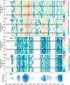 |
Fig. A.1 Occurrence phase of the NB emissions in SKR longitude systems. Panels (a)-(b) give the northern and southern hemisphere 5 kHz NB emission occurrences in the SKR derived longitude systems (SLS5-N and SLS5-S). The color code represents the averaged occurrence of the NB emissions in the corresponding time and longitude. The solid and dashed black lines represent the mean and one sigma deviation values derived in Fig. 4. Two rotation periods of the results are shown in each panel in order to give clearer illustrations. The northern and southern events of both the 5 kHz NB and 20 kHz NB are simply separated by choosing Lat > 0° or Lat <0°. Panels (c)-(d) present the northern and southern hemisphere 20 kHz NB emission occurrences in the SKR derived longitude systems (SLS5-N and SLS5-S). Panel (e) shows the Cassini latitude from 2004 to 2017. |
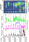 |
Fig. A.2 Phase-lock observation in the same format as Fig. 5 in the manuscript. The observation is from 29 August 2012 to 2 September 2012. The blue dashed line shows the “disturbed phase lock” or “loss of phase lock” feature. The occurrence sequence of the radio component changes from the “typical” phase-lock sequence. The “disturbed” feature could be due to the external influence of the magnetosphere, as indicated by the later enhancement of the SKR. |
References
- Andrews, D. J., Bunce, E. J., Cowley, S. W. H., et al. 2008, J. Geophys. Res. Space Phys., 113, A09205 [NASA ADS] [Google Scholar]
- Andrews, D. J., Coates, A. J., Cowley, S. W., et al. 2010, J. Geophys. Res. Space Phys., 115, 1 [Google Scholar]
- Andrews, D. J., Cowley, S. W. H., Dougherty, M. K., et al. 2012, J. Geophys. Res. Space Phys., 117, A04224 [NASA ADS] [CrossRef] [Google Scholar]
- Andrews, D. J., Cowley, S. W. H., Provan, G., et al. 2019, J. Geophys. Res. Space Phys., 124, 8361 [NASA ADS] [CrossRef] [Google Scholar]
- Azari, A. R., Jia, X., Liemohn, M. W., et al. 2019, J. Geophys. Res.: Space Phys., 124, 1806 [NASA ADS] [CrossRef] [Google Scholar]
- Benson, R. F., Webb, P. A., Green, J. L., et al. 2006, Active Wave Experiments in Space Plasmas: The Z Mode, eds. J. W. LaBelle, & R. A. Treumann (Berlin, Heidelberg: Springer Berlin Heidelberg), 3 [Google Scholar]
- Bradley, T. J., Cowley, S. W. H., Provan, G., et al. 2018, J. Geophys. Res. Space Phys., 123, 3602 [CrossRef] [Google Scholar]
- Bunce, E. J., Cowley, S. W., Wright, D. M., et al. 2005, Geophys. Res. Lett., 32, 1 [NASA ADS] [CrossRef] [Google Scholar]
- Burch, J. L., Goldstein, J., Mokashi, P., et al. 2008, Geophys. Res. Lett., 35, 2 [CrossRef] [Google Scholar]
- Calvert, W. 1995, J. Geophys. Res. Space Phys., 100, 17491 [NASA ADS] [CrossRef] [Google Scholar]
- Carbary, J. F., Mitchell, D. G., Brandt, P., Paranicas, C., & Krimigis, S. M. 2008a, Geophys. Res. Lett., 35, L07102 [NASA ADS] [Google Scholar]
- Carbary, J. F., Mitchell, D. G., Brandt, P., Roelof, E. C., & Krimigis, S. M. 2008b, Geophys. Res. Lett., 35, L24101 [NASA ADS] [Google Scholar]
- Carpenter, D. L., Spasojevic, M. A., Bell, T. F., et al. 2002, J. Geophys. Res. Space Phys., 107, SMP 22 [CrossRef] [Google Scholar]
- Cecconi, B., & Zarka, P. 2005, Radio Sci., 40, 1 [NASA ADS] [CrossRef] [Google Scholar]
- Cecconi, B., Lamy, L., & Zarka, P. 2017a, Cassini/RPWS/HFR LESIA/KronosN2 Data Collection (Version 1.0) [Google Scholar]
- Cecconi, B., Lamy, L., & Zarka, P. 2017b, Cassini/RPWS/HFR LESIA/KronosN3d Data Collection (Version 1.0) [Google Scholar]
- Clarke, K. E., André, N., Andrews, D. J., et al. 2006, Geophys. Res. Lett., 33, L23104 [NASA ADS] [CrossRef] [Google Scholar]
- Clarke, K. E., Andrews, D. J., Coates, A. J., Cowley, S. W. H., & Masters, A. 2010, J. Geophys. Res. Space Phys., 115, A05202 [NASA ADS] [Google Scholar]
- Cowley, S. W. H., & Provan, G. 2013, J. Geophys. Res.: Space Phys., 118, 7246 [NASA ADS] [CrossRef] [Google Scholar]
- Cowley, S. W. H., & Provan, G. 2017, J. Geophys. Res.: Space Phys., 122, 6049 [CrossRef] [Google Scholar]
- Cowley, S. W. H., Bunce, E. J., & O’Rourke, J. M. 2004, J. Geophys. Res.: Space Phys., 109, A02201 [NASA ADS] [CrossRef] [Google Scholar]
- Cowley, S. W. H., Achilleos, N., Bradley, T. J., et al. 2020, J. Geophys. Res. Space Phys., 125, e2020JA028247 [CrossRef] [Google Scholar]
- Davies, M., Abalakin, V., Brahic, A., et al. 1992, Celest. Mech. Dyn. Astron., 53, 377 [NASA ADS] [CrossRef] [Google Scholar]
- Desch, M. D., & Kaiser, M. L. 1981, Geophys. Res. Lett., 8, 253 [NASA ADS] [CrossRef] [Google Scholar]
- Eckersley, T. L. 1933, Proc. Roy. Soc. London Ser. A, 141, 697 [NASA ADS] [CrossRef] [Google Scholar]
- Ellis, G. R. 1956, J. Atmos. Terrestrial Phys., 8, 43 [NASA ADS] [CrossRef] [Google Scholar]
- Espinosa, S. A., & Dougherty, M. K. 2000, Geophys. Res. Lett., 27, 2785 [NASA ADS] [CrossRef] [Google Scholar]
- Fischer, G., Gurnett, D., Kurth, W., Ye, S. Y., & Groene, J. 2015, Icarus, 254, 72 [NASA ADS] [CrossRef] [Google Scholar]
- Goldreich, P., & Farmer, A. J. 2007, J. Geophys. Res. Space Phys., 112, A05225 [NASA ADS] [CrossRef] [Google Scholar]
- Gurnett, D. A., Kurth, W. S., & Scarf, F. L. 1981, Nature, 292, 733 [NASA ADS] [CrossRef] [Google Scholar]
- Gurnett, D. A., Kurth, W. S., Kirchner, D. L., et al. 2004, Space Sci. Rev., 114, 395 [NASA ADS] [CrossRef] [Google Scholar]
- Gurnett, D. A., Lecacheux, A., Kurth, W. S., et al. 2009a, Geophys. Res. Lett., 36, L16102 [NASA ADS] [Google Scholar]
- Gurnett, D. A., Persoon, A. M., Groene, J. B., et al. 2009b, Geophys. Res. Lett., 36, L21108 [NASA ADS] [Google Scholar]
- Gurnett, D. A., Groene, J. B., Persoon, A. M., et al. 2010, Geophys. Res. Lett., 37, L24101 [NASA ADS] [Google Scholar]
- Hill, T. W. 1976, Planet. Space Sci., 24, 1151 [NASA ADS] [CrossRef] [Google Scholar]
- Hunt, G. J., Cowley, S. W. H., Provan, G., et al. 2014, J. Geophys. Res. Space Phys., 119, 9847 [NASA ADS] [CrossRef] [Google Scholar]
- Hunt, G. J., Cowley, S. W. H., Provan, G., et al. 2015, J. Geophys. Res. Space Phys., 120, 7552 [NASA ADS] [CrossRef] [Google Scholar]
- Jackman, C. M., Lamy, L., Freeman, M. P., et al. 2009, J. Geophys. Res.: Space Phys., 114, A08211 [NASA ADS] [Google Scholar]
- Jackman, C. M., Arridge, C. S., Slavin, J. A., et al. 2010, J. Geophys. Res. Space Phys., 115, A10240 [NASA ADS] [CrossRef] [Google Scholar]
- Jia, X., Hansen, K. C., Gombosi, T. I., et al. 2012, J. Geophys. Res. Space Phys., 117, A05225 [NASA ADS] [Google Scholar]
- Kaiser, M. L., Desch, M. D., Warwick, J. W., & Pearce, J. B. 1980, Science, 209, 1238 [CrossRef] [Google Scholar]
- Khurana, K. K., Mitchell, D. G., Arridge, C. S., et al. 2009, J. Geophys. Res. Space Phys., 114, A02211 [NASA ADS] [CrossRef] [Google Scholar]
- LaBelle, J., & Treumann, R. A. 2002, Space Sci. Rev., 101, 295 [NASA ADS] [CrossRef] [Google Scholar]
- Lamy, L. 2011, in Proceeding Planetary Radio Emissions VII, 39 [NASA ADS] [CrossRef] [Google Scholar]
- Lamy, L., Cecconi, B., Prangé, R., et al. 2009, J. Geophys. Res.: Space Phys., 114, A10212 [NASA ADS] [Google Scholar]
- Lamy, L., Zarka, P., Cecconi, B., et al. 2018, Science, 362, 6410 [CrossRef] [Google Scholar]
- Menietti, J. D., Mutel, R. L., Schippers, P., et al. 2011, J. Geophys. Res. Space Phys., 116, A12222 [NASA ADS] [Google Scholar]
- Menietti, J. D., Yoon, P. H., Pisa, D., et al. 2019, J. Geophys. Res.: Space Phys., 124, 5709 [NASA ADS] [CrossRef] [Google Scholar]
- Mitchell, D. G., Brandt, P. C., Carbary, J. F., et al. 2015, Injection, Interchange, and Reconnection (American Geophysical Union (AGU)), 327 [Google Scholar]
- Nichols, J. D., Clarke, J. T., Cowley, S. W. H., et al. 2008, J. Geophys. Res. Space Phys., 113, A11205 [NASA ADS] [CrossRef] [Google Scholar]
- Paranicas, C., Mitchell, D. G., Roelof, E. C., et al. 2005, Geophys. Res. Lett., 32, L21101 [NASA ADS] [Google Scholar]
- Persoon, A. M., Kurth, W. S., Gurnett, D. A., et al. 2020, J. Geophys. Res. Space Phys., 125, e2019JA027545 [CrossRef] [Google Scholar]
- Provan, G., Andrews, D. J., Arridge, C. S., et al. 2009, J. Geophys. Res. Space Phys., 114, A02225 [NASA ADS] [Google Scholar]
- Provan, G., Andrews, D. J., Cecconi, B., et al. 2011, J. Geophys. Res.: Space Phys., 116, A04225 [Google Scholar]
- Provan, G., Cowley, S. W. H., Sandhu, J., Andrews, D. J., & Dougherty, M. K. 2013, J. Geophys. Res. Space Phys., 118, 3243 [NASA ADS] [CrossRef] [Google Scholar]
- Provan, G., Lamy, L., Cowley, S. W. H., & Dougherty, M. K. 2014, J. Geophys. Res. Space Phys., 119, 7380 [NASA ADS] [CrossRef] [Google Scholar]
- Provan, G., Cowley, S. W. H., Lamy, L., et al. 2016, J. Geophys. Res.: Space Phys., 121, 9829 [NASA ADS] [CrossRef] [Google Scholar]
- Provan, G., Cowley, S. W. H., Bradley, T. J., et al. 2018, J. Geophys. Res. Space Phys., 123, 3859 [NASA ADS] [CrossRef] [Google Scholar]
- Provan, G., Cowley, S. W. H., Bradley, T. J., et al. 2019, J. Geophys. Res. Space Phys., 124, 8814 [CrossRef] [Google Scholar]
- Provan, G., Cowley, S. W. H., Bunce, E. J., et al. 2021, J. Geophys. Res. Space Phys., 126, e2021JA029332 [NASA ADS] [CrossRef] [Google Scholar]
- Radioti, A., Yao, Z., Grodent, D., et al. 2019, ApJ, 885, L16 [NASA ADS] [CrossRef] [Google Scholar]
- Reed, J. J., Jackman, C. M., Lamy, L., Kurth, W. S., & Whiter, D. K. 2018, J. Geophys. Res. Space Phys., 123, 443 [CrossRef] [Google Scholar]
- Reinisch, B. W., Huang, X., Song, P., et al. 2001, Geophys. Res. Lett., 28, 4521 [NASA ADS] [CrossRef] [Google Scholar]
- Scargle, J. 1982, ApJ, 263, 835 [NASA ADS] [CrossRef] [Google Scholar]
- Smith, C. G. A. 2011, MNRAS, 410, 2315 [NASA ADS] [CrossRef] [Google Scholar]
- Southwood, D. J., & Kivelson, M. G. 2009, J. Geophys. Res. Space Phys., 114, A09201 [NASA ADS] [CrossRef] [Google Scholar]
- Southwood, D. J., & Cowley, S. W. H. 2014, J. Geophys. Res. Space Phys., 119, 1563 [NASA ADS] [CrossRef] [Google Scholar]
- Wang, Z., Gurnett, D. A., Fischer, G., et al. 2010, J. Geophys. Res.: Space Phys., 115, A06213 [NASA ADS] [Google Scholar]
- Warwick, J. W., Pearce, J. B., Evans, D. R., et al. 1981, Science, 212, 239 [NASA ADS] [CrossRef] [Google Scholar]
- Wing, S., Brandt, P. C., Mitchell, D. G., et al. 2020, AJ, 159, 249 [CrossRef] [Google Scholar]
- Wing, S., Thomsen, M. F., Johnson, J. R., et al. 2022, ApJ, 937, 42 [NASA ADS] [CrossRef] [Google Scholar]
- Winglee, R. M., Kidder, A., Harnett, E., et al. 2013, J. Geophys. Res.: Space Phys., 118, 4253 [CrossRef] [Google Scholar]
- Wu, S., Ye, S., Georg, F., et al. 2021, ApJ, 918, 1 [NASA ADS] [CrossRef] [Google Scholar]
- Wu, S. Y., Ye, S. Y., Fischer, G., et al. 2022, Geophys. Res. Lett., 49, e2021GL096990 [NASA ADS] [CrossRef] [Google Scholar]
- Wu, S., Zarka, P., Lamy, L., et al. 2023, J. Geophys. Res. Space Phys., 128, e2023JA031287 [NASA ADS] [CrossRef] [Google Scholar]
- Ye, S.-Y., Gurnett, D. A., Fischer, G., et al. 2009, J. Geophys. Res.: Space Phys., 114, A06219 [NASA ADS] [Google Scholar]
- Ye, S.-Y., Gurnett, D. A., Groene, J. B., Wang, Z., & Kurth, W. S. 2010a, J. Geophys. Res.: Space Phys., 115, A12258 [NASA ADS] [Google Scholar]
- Ye, S.-Y., Menietti, J. D., Fischer, G., et al. 2010b, J. Geophys. Res.: Space Phys., 115, A08228 [NASA ADS] [Google Scholar]
- Ye, S.-Y., Fischer, G., Kurth, W. S., Menietti, J. D., & Gurnett, D. A. 2016, J. Geophys. Res. Space Phys., 121, 11711 [Google Scholar]
- Ye, S.-Y., Fischer, G., Kurth, W. S., Menietti, J. D., & Gurnett, D. A. 2018, Geophys. Res. Lett., 45, 7297 [NASA ADS] [CrossRef] [Google Scholar]
All Figures
|
Fig. 1 Clock-like modulation of NB emissions. Panel a: clock or rotating beam test for 5 kHz NB. The horizontal axis of ω0 encompasses the assumed modulation rates of 785 to 830° per day, which was chosen to be near the rotation rate of Saturn (10.7 hours = 807° per day). The vertical axis is the fitted peak-to-peak modulation power giving the fitted peak power of the 240-day time series under the assumption of each ω0. The two solid lines show the modulation rates of 5 kHz NB emissions under the assumption of a clock-like source (red) and a rotating beam source (blue). Panel b: similar format as panel a but for 20 kHz NB emissions. The black dashed lines mark the modulation rate in the same 240-day window derived from the SKR intensities. The 5 kHz and 20 kHz NB time series used in this window are not separated into two hemispheres according to latitude. |
| In the text | |
|
Fig. 2 North-south asymmetry test of the 20 kHz NB emissions. Panel a: modulation rate of the 20 kHz NB emissions in the northern hemisphere, similar to Fig. 1. Panel b: similar format as panel a but for the southern hemisphere. The 20 kHz NB time series used in this window is separated into two hemispheres according to the latitudes (Lat: >10° and < −10°). |
| In the text | |
|
Fig. 3 Least-squares spectral analysis spectrograms of Saturn radio emissions from 2004 to 2018. The color-coded spectrograms show the modulation power as a function of universal time in the horizontal axis and the modulation rate in the vertical axis. Panels a–d respectively show the results for the northern hemisphere SKR, the southern hemisphere SKR, the 5 kHz NB emissions (in both hemispheres), and the 20 kHz NB emissions (in both hemispheres). Panel e shows the Cassini latitudes during its Saturn orbital journey. The green and orange lines are the northern and southern SKR periods as derived by Ye et al. (2018). The blue and pink lines are the northern and southern PPO periods as derived by Provan et al. (2013, 2016, 2019). |
| In the text | |
|
Fig. 4 Clock-phase difference of Saturn radio emissions. Panel a: relative phase between SKR and 5 kHz NB emissions in the northern (black) and southern (pink) hemispheres. Panel b: relative phase between 5 kHz NB emissions and 20 kHz NB emissions. Panel c: relative phase between SKR and 20 kHz NB emissions. |
| In the text | |
|
Fig. 5 Relative phase of the Saturn radio emissions. Panel a: Cassini RPWS wave electric field spectrogram. The horizontal white dashed lines mark the frequencies of 71.2 kHz (corresponding to SKR), 15 kHz (corresponding to 20 kHz NB), and 5.1 kHz (corresponding to 5 kHz NB), which are used in the following panels to plot the frequency intensity versus time variation. The blue, pink, and black arrows in panel a indicate the three radio emissions. Panels b–d: spectral density in units of dB above the background. The oblique red dashed lines depict the rough phase relation between the three radio emissions. The peaks marked by the oblique red dashed lines correspond to the blue, pink, and black arrows in panel a, which correspond to the main emissions of SKR, 5 kHz NB, and 20 kHz NB. The black shaded regions in panels b–d indicate the regions that are polluted by the low-frequency extensions of SKR. The relatively constant relations shown suggest a phase-lock situation. |
| In the text | |
|
Fig. A.1 Occurrence phase of the NB emissions in SKR longitude systems. Panels (a)-(b) give the northern and southern hemisphere 5 kHz NB emission occurrences in the SKR derived longitude systems (SLS5-N and SLS5-S). The color code represents the averaged occurrence of the NB emissions in the corresponding time and longitude. The solid and dashed black lines represent the mean and one sigma deviation values derived in Fig. 4. Two rotation periods of the results are shown in each panel in order to give clearer illustrations. The northern and southern events of both the 5 kHz NB and 20 kHz NB are simply separated by choosing Lat > 0° or Lat <0°. Panels (c)-(d) present the northern and southern hemisphere 20 kHz NB emission occurrences in the SKR derived longitude systems (SLS5-N and SLS5-S). Panel (e) shows the Cassini latitude from 2004 to 2017. |
| In the text | |
|
Fig. A.2 Phase-lock observation in the same format as Fig. 5 in the manuscript. The observation is from 29 August 2012 to 2 September 2012. The blue dashed line shows the “disturbed phase lock” or “loss of phase lock” feature. The occurrence sequence of the radio component changes from the “typical” phase-lock sequence. The “disturbed” feature could be due to the external influence of the magnetosphere, as indicated by the later enhancement of the SKR. |
| In the text | |
Current usage metrics show cumulative count of Article Views (full-text article views including HTML views, PDF and ePub downloads, according to the available data) and Abstracts Views on Vision4Press platform.
Data correspond to usage on the plateform after 2015. The current usage metrics is available 48-96 hours after online publication and is updated daily on week days.
Initial download of the metrics may take a while.