| Issue |
A&A
Volume 680, December 2023
|
|
|---|---|---|
| Article Number | A69 | |
| Number of page(s) | 9 | |
| Section | Extragalactic astronomy | |
| DOI | https://doi.org/10.1051/0004-6361/202346916 | |
| Published online | 12 December 2023 | |
A fast test for the identification and confirmation of massive black hole binaries
1
Università degli Studi di Milano-Bicocca, Piazza della Scienza 3, 20126 Milano, Italy
e-mail: This email address is being protected from spambots. You need JavaScript enabled to view it.
2
INFN – Sezione di Milano-Bicocca, Piazza della Scienza 3, 20126 Milano, Italy
3
INAF – Osservatorio Astronomico di Brera, Via Brera 20, 20121 Milano, Italy
4
DiSAT – Università degli Studi dell’Insubria, Via Valleggio 11, 22100 Como, Italy
5
Dipartimento di Fisica “E. Fermi”, Università di Pisa, 56127 Pisa, Italy
6
Istituto Nazionale di Fisica Nucleare, Sezione di Pisa, 56127 Pisa, Italy
7
NAF – Osservatorio di Astrofisica e Scienza dello Spazio di Bologna, Via Gobetti 93/3, 40129 Bologna, Italy
Received:
16
May
2023
Accepted:
8
October
2023
Abstract
We present a new observational test to identify massive black hole binaries in large multi-epoch spectroscopical catalogues and to confirm already proposed binary candidates. The test is tailored for binaries with large enough separations to allow each black hole to retain its own broad line region (BLR). Within this limit, the fast variability of active galactic nuclei (AGN) typically observed over months cannot be associated to the much longer binary period and is assumed (as for the case of single black holes) to be the consequence of the evolution of the innermost regions of the two accretion discs. A simple analysis of the cross-correlation between different parts of individual broad emission lines can therefore be used to identify the presence of two massive black holes whose continua vary independently of each other. Our analysis indicates that, to be less affected by the noise in the spectra, the broad lines should be divided into two parts of almost equal flux. This ensures that, in the single massive black hole scenario, the cross-correlation will always be strong. With monitoring campaigns similar to those performed for reverberation mapping studies, inversely, a binary can show any value of the cross-correlation and can therefore be distinguished from a standard AGN. This new test can be performed over timescales that are orders of magnitude shorter than the alternative tests already discussed in the literature, and can be a powerful complement to the massive black hole binary search strategies already in place.
Key words: accretion / accretion disks / galaxies: interactions / quasars: supermassive black holes / quasars: emission lines / techniques: spectroscopic
© The Authors 2023
 Open Access article, published by EDP Sciences, under the terms of the Creative Commons Attribution License (https://creativecommons.org/licenses/by/4.0), which permits unrestricted use, distribution, and reproduction in any medium, provided the original work is properly cited.
This article is published in open access under the Subscribe to Open model. This email address is being protected from spambots. You need JavaScript enabled to view it. to support open access publication.
1. Introduction
Gravitationally bound massive black hole binaries (MBHBs) are the outcome of galaxy mergers, and were originally predicted by Begelman et al. (1980). They are among the loudest sources of gravitational waves (GWs) detectable with current pulsar timing array (PTA) campaigns (Verbiest et al. 2016) and by future space-based gravitational wave interferometers (e.g. LISA; Amaro-Seoane et al. 2017, 2023). The GW background generated by MBHBs, and the rate of detectable binary coalescence, are still quite uncertain. This is partly a consequence of the uncertainties on the efficiency of MBH pairing during the early stages of galaxy mergers (Fiacconi et al. 2013; del Valle et al. 2015; Tamburello et al. 2017; Souza Lima et al. 2017; Bortolas et al. 2020, 2022). The electromagnetic (EM) identification of a sample of already bound MBH binaries would therefore greatly reduce the uncertainties on the signals observable with both PTA and LISA.
To date, unequivocal observational confirmation of an MBHB has not yet been found. The only spatially resolved MBHB candidate is 0402+379 (Rodriguez et al. 2009; Burke-Spolaor 2011), which has two flat-spectrum radio cores with a projected separation of ≈7 pc.
At smaller, spatially unresolved scales, MBHBs have been consistently searched for either through peculiar spectral features (Tsalmantza et al. 2011; Eracleous et al. 2012; Ju et al. 2013; Shen et al. 2013; Wang et al. 2017) or through photometric variability (Valtonen et al. 2008; Ackermann et al. 2015; Graham et al. 2015; Li et al. 2016, 2019; Charisi et al. 2016; Sandrinelli et al. 2016, 2018; Severgnini et al. 2018; Liu et al. 2019; Chen et al. 2020). These two search strategies target MBHBs at different separations. The spectroscopic approach assumes that the broad line region (BLR) of at least one of the binary components does not extend beyond its MBH Roche radius. Therefore, by sharing the same kinematics as the MBH, the broad emission lines (BELs) are shifted in frequency with respect to the host galaxy rest frame and evolve in time over a binary orbital period τorb. The constraint on the size of the BLR can be translated into a constraint on the minimum binary separation, which is of the order of ∼0.1 pc for a 108 M⊙ MBH accreting at one-tenth of its Eddington ratio (see Sect. 2 for more details).
At smaller separations, the BLR is either truncated by the time-dependent binary potential (Montuori et al. 2011) or shared by both MBHs and comoving with the MBHB centre of mass. Theoretical studies predict periodic variability on timescales of ∼τorb, either associated with the periodic fueling from the circumbinary material (e.g. Hayasaki et al. 2008) or with the Doppler boosting of the emission for very close binaries (D’Orazio et al. 2015). At close separations, such timescales can be as short as ≲1 yr, allowing observational searches in current and future multi-epoch observations (see Graham et al. 2015; Charisi et al. 2016; Liu et al. 2019; Chen et al. 2020, and references therein).
Nevertheless, a major problem is that all of the above-mentioned features used to identify MBHB candidates can have alternative explanations (see Dotti et al. 2023, for an overview of the possible alternative interpretations). Theoretical prediction of clear and unique observational features associated with MBHBs is therefore needed in order to test the actual binary nature of both small- (selected through their variability) and large-scale (spectroscopically identified) MBHB candidates. Some tests have recently been proposed for the small-scale MBHB candidates, including the possibility of periodic gravitational lensing from the companion of the active component of the MBHB (for binaries observed nearly edge-on, see e.g. D’Orazio & Di Stefano 2018; Davelaar & Haiman 2022a,b) and periodic evolution of the polarisation fraction and angle (Dotti et al. 2022).
For MBHBs at larger separations (e.g. Gaskell 1996; Eracleous et al. 1997), a straightforward test consists in observing the expected Doppler drift in the BEL profiles according to the motion of the active component (or components, if both MBHs are active) of the binary with a τorb period (e.g. Gaskell 1996; Eracleous et al. 1997). A conclusive test would require following the system spectroscopically for ∼τorb. However, at these scales, τorb can be as high as ≳10 − 100 yr (see Sect. 2), making such a test (dubbed slow periodicity test (SPT) hereafter) challenging and unpractical for some of the candidates (see e.g. Eracleous et al. 2012; Decarli et al. 2013; Runnoe et al. 2017).
In this paper, we propose a new test for the same large-separation binary candidates based on the assumption that, at such large separations, the short-timescale (≲1 day) intrinsic accretion variability is unrelated to the binary period, and that, when both MBHs are active, their variability patterns are uncorrelated. Each BLR reverberates to the varying continuum of its MBH (e.g. Blandford & McKee 1982). As we argue in the following, dividing the BELs into two components (one “red” and one “blue”, which together account for the total flux in the BEL) and cross-correlating the time-evolution of their fluxes can provide a means to identify MBHBs. Indeed, in the binary scenario, each observed BEL would be composed into two different broad lines, each with a different velocity offset with respect to the galaxy rest frame, and with the two components varying independently. In this scenario, the cross-correlation between the blue and red parts of the BELs can be significantly smaller with respect to the case of an AGN powered by a single MBH, as long as the velocity offset is not negligible (i.e. each component associated to one of the MBHs contributes significantly to one of the blue or red parts of the global BEL). This implies that our test becomes decreasingly effective for larger and larger binary separations, with a cross-correlation between the two different parts of the BEL getting closer and closer to the high values expected for single MBHSs, and failing to detect any true binary for close-to-zero relative line-of-sight velocity between the two MBHs (see Sect. 4). However, while other proposed spectroscopical tests are expected to fail when the velocity shift between the two components is equal to their width (e.g. Shen & Loeb 2010), in Sect. 4 we demonstrate that our test can still identify binaries at larger separations and smaller velocity shifts, including binaries with periods of up to ∼1000 yr.
Our proposed method can be thought of as a simplified version of the tests proposed by Wang et al. (2018), Songsheng et al. (2020), in which a catalogue of two-dimensional transfer functions (TFs) for different binaries is constructed and compared to the full TF of a candidate binary. While our method is clearly less sensitive to the details of the BEL profile variability, it provides fast and quantitative verification of the binary nature of the candidate, even when the quality of the data is suboptimal for constraining the details of the TF.
The clearest advantage of our new test (dubbed fast uncorrelated variability test; FUVT) is that it can be performed over timescales comparable to the typical duration of the reverberation mapping (RM) campaigns (e.g. Bentz et al. 2009a), which is usually smaller than 1 yr (down to weeks, and orders of magnitude smaller than τorb). A second advantage is that, while FUVT can be applied to already identified MBHB candidates with shifted asymmetric or double-peaked BELs, it can also be used to identify new binaries with apparently “standard” BELs in large multi-epoch samples of AGNs.
This paper is organised as follows: in Sect. 2 we describe the timescales required by FUVT and its range of applicability in terms of intrinsic MBHB properties; in Sect. 3 we describe how the FUVT is structured, and we present the results of its application to a real sample of type I AGN (sample I hereafter) studied using RM; in Sect. 4 we explain how we constructed a mock catalogue of MBHBs (sample II) starting from sample I, and present the results of the application of FUVT to the new binary sample; we then conclude with Sect. 5, summarising the main results of our study, describing the advantages and disadvantages of FUVT with respect to SPT, and discussing how future observations can further strengthen the test results.
2. Analytical estimates of FUVT range of applicability
As mentioned in Sect. 1, both SPT and FUVT assume that both the BLRs are bound to and comoving with the individual components of the binary. The BLR radius depends on the BEL we are focusing on and on the luminosities of the accreting MBHs. For the broad Hβ line used in the following, the BLR radius is (Bentz et al. 2009b)
 (1)
(1)
where λLλ, 5100 is the monocromatic luminosity of the AGN continuum at 5100 Å. Assuming that the bolometric luminosity is Lbol ≈ 9 λLλ, 5100 (Kaspi et al. 2000), we can express Eq. (1) as a function of the individual MBH mass M and its Eddington ratio fEdd = Lbol/LEdd:
 (2)
(2)
It is required that this radius be smaller than the Roche lobe radius of each individual MBH (Montuori et al. 2011). For the test to work, the fluxes from the two accretion discs (and therefore the BLR radii) have to be comparable. For this reason, the minimum separation between the two MBHs is set by the Roche lobe of the secondary MBH, which for circular binaries is (Eggleton 1983)
 (3)
(3)
where a is the separation between the two MBHs and q = M2/M1 is the ratio between the secondary and the primary masses.
The minimum separation of the binary and, assuming circular Keplerian orbits, the minimum value of τorb for which both SPT and FUVT are applicable is obtained by equating Eqs. (2) and (3):
![Mathematical equation: $$ \begin{aligned} \tau _{\rm orb, min} \approx &200 \, \mathrm{yr} \, f_{\rm Edd, 2}^{0.78}\, \left(\frac{M_2}{10^6\,M_\odot }\right)^{0.28}\nonumber \\& \sqrt{\frac{[0.6\, q^{2/3}\, + \, \ln (1+q^{1/3})]^3}{q \, (1+q)}}, \end{aligned} $$](/articles/aa/full_html/2023/12/aa46916-23/aa46916-23-eq4.gif) (4)
(4)
where fEdd, 2 is the Eddington ratio of the secondary. It is interesting to note that τorb, min has a stronger dependence on fEdd, 2 than on M2. Therefore, at fixed luminosity, shorter minimum periods are expected for higher MBH masses. Similarly to the spectroscopic MBHB candidates proposed to date (e.g. Tsalmantza et al. 2011; Eracleous et al. 2012), secondary MBHs of 108 M⊙ could be in binaries with minimum periods of as small as ∼27 yr (see also Decarli et al. 2013; Runnoe et al. 2017) if accreting at fEdd, 2 = 0.01, that is, with the same bolometric luminosity as an MBH of 106 M⊙ accreting at its Eddington limit.
However, we note that for disc-like BLRs, the region within which circular orbits around a single MBH are stable is sizeably smaller (by a factor of ≈4 − 5) than the Roche lobe (e.g. Eggleton 1983; Runnoe et al. 2015). On top of this consideration, gas at distances of > RB − Hβ contribute to the central part of the broad Hβ line, and, if the binary separation is too small, such a contribution would be lost and the line would acquire a “boxy” profile1. In the following, we consider binaries with periods corresponding to BLR sizes similar to the secondary Roche lobe, as well as binaries with significantly larger periods, for which a stable disc-like BLR can survive around each of the two MBHs (see Sect. 4).
Finally, the typical timescale for the Hβ reverberation to the change of the continuum can be estimated as τB − Hβ = RB − Hβ/c (where c is the speed of light). This timescale was evaluated using RM and ranges from days to months depending on the luminosity of the accreting MBH. However, RM studies typically require longer durations – even for ∼106 M⊙ MBHs – due to the need for sufficiently long baselines and sufficiently varying continua to allow for the test. As a consequence, the typical timescales needed to probe the variability both in the continuum and in the BELs are of the order of weeks to months (Bentz et al. 2009a).
3. FUVT description and results on a control sample of single MBHs
We apply FUVT to nine AGN for which τB − Hβ (and therefore masses) were obtained by Bentz et al. (2009a): Mrk 142, SBS 1116+583A, Arp 151, Mrk 1310, Mrk 202, NGC 4253, NGC 4748, NGC 5548, and NGC 6814. We assume, as a working hypothesis, that the whole sample is composed of only bona fide single MBHs, and use it as a comparison for the mock binary sample described in the following section. Nevertheless, we stress that at least one of the AGN in sample I (NGC 5548) has been proposed as a binary candidate (Li et al. 2016) based on the variability of the periodic modulation of its broad Hβ line.
For all AGN, Bentz et al. (2009a) estimated delays between the continuum and the broad Hβ of between 2 and 7 days and masses in the range of 1 − 7 × 10⁶ M⊙, with the exception of NGC 6814, which has a mass ≈1.85 × 10⁷ M⊙, and NGC 5548, which has a mass of 8.2 × 10⁷ M⊙ (see Bentz et al. 2009a, for additional details on the properties of the single AGNs).
For our analysis, we used scaled spectra released by these latter authors after the application of a renormalisation used to set the flux of all spectra to a consistent scale. For every AGN, we removed the mean spectrum (averaged over all the observations) and worked on the variable part of the spectrum only, which is dominated by the AGN continua and the BELs. We then removed the AGN continuum by fitting a straight line to the spectrum near the Hβ BEL using the same wavelength intervals as those used in Bentz et al. (2009a)2.
For each AGN, we then computed the root mean square (RMS) spectrum. We used it to identify seven  dividing the RMS broad Hβ into eight parts of equal flux3. For each
  in each spectrum, we divided the Hβ BEL into two components, a red one and a blue one (r-Hβ and b-Hβ, for wavelengths longer and shorter than
  , respectively). We then computed the light curves of the r-Hβ and b-Hβ components, and performed the cross-correlation between the two, allowing for a small time-shift τshift in the [−10 days, 10 days] interval to take into account different reverberation times for different parts of the broad lines (due to e.g. the inflowing or outflowing BLR dynamics; e.g. Bentz et al. 2009a). More specifically, we follow the standard RM practice of first using one light curve and interpolating the other, before swapping the two and repeating the exercise. The average cross-correlation is then used, and the uncertainties on the cross-correlation and τshift are estimated using the public PYTHON version (Sun et al. 2018)4 of the Monte Carlo code discussed in Peterson et al. (1998, 2004).
For each AGN and each  we measure
  , that is, the maximum value of the r-Hβ–b-Hβ cross-correlation, and its uncertainties. The
  obtained following this procedure are shown in Fig. 1 for NGC 4748. The peak of
  (
( hereafter)5 corresponds to the
  threshold dividing the broad Hβ line into two parts of equal flux, while the cross-correlation decreases significantly (and its uncertainties increase) when moving
  towards the line wings, which are more affected by the noise in the spectra. More generally, in the sample, the values of
  are comparable to or slightly higher than the peak of the cross-correlations between the whole broad Hβ and the photometric B and V light curves shown in Bentz et al. (2009a). The trends discussed for NGC 4748 are common for all nine of the AGN we examined:
  is always found in the bulk of the line (hereby defined as the region in between the third and the fifth values of
  , i.e. when the least luminous part of the BEL has at least three-eighths of the total BEL flux), and it is always ≳0.756.
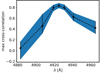 |
Fig. 1. NGC 4748: Maximum value of the cross correlation between the blue and red parts of the broad Hβ line as a function of the dividing wavelength |

4. Application of FUVT to mock MBHBs
We apply FUVT to mock equal-mass MBHBs generated by duplicating the temporal series of spectra of each of the nine single MBHs discussed above. One of the copies is shifted in time by half of the observational period (assuming periodic boundary conditions, as done in standard reverberation mapping studies). As the magnitude of the time-shift τshift in the test is constrained to be smaller than 10 days, such a shift makes the evolution of the two series of spectra independent. The original and shifted light curves (blue and red lines) of the whole Hβ for NGC 4748, together with the sum of the two (green line), mimicking the light curve of a MBHB, are shown in Fig. 27.
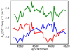 |
Fig. 2. NGC 4748: Original light curve of the entire Hβ line (blue line), the same light curve shifted by half of the observational period (with periodic boundary conditions, red line), and the sum of the two (rigidly shifted towards lower fluxes for visualisation purposes, green line), mimicking a MBHB whose components evolve independently on short timescales. |
The two series of spectra are then shifted in frequency by the same amount towards higher and lower wavelengths, respectively. The wavelength shifts are chosen in order to mimic circular MBHBs with periods of τorb = 50, 100, 300, and 1000 yr, observed close to edge-on at the orbital phase that would maximise the Doppler effect. We chose such a configuration to check whether or not the test succeeds in identifying binaries in the most favourable scenario. Different configurations would result in smaller shifts between the two independent components of the BEL, and could in principle result in a missed detection. We note that, while all four periods fulfill the criterion set in Eq. (4), τorb = 50, 100 would correspond to separations at which a sizable part of a disc-like BLR would be unstable. Furthermore, for those periods, the outer parts of the BLR would be removed, resulting in a more “boxy” profile of each BEL component (see e.g. Nguyen et al. 2019), while only a few of the AGN discussed in Sect. 3 have a boxy broad Hβ. For these reasons, hereafter we refer to binaries with τorb = 300 and 1000 yr as “solid” binaries, while keeping the τorb = 50 and 100 yr binaries to highlight how the performance of our test scales with the orbital period and to account for possible alternative geometries and dynamics of the BLR.
We then add the two series up (adding the original errors in quadrature for each wavelength bin), obtaining four new mock MBHBs for each original MBH, for a grand total of 36 mock MBHBs. The upper panel of Fig. 3 shows an example of a mock MBHB spectrum based on the observations of NGC 4748 – without the application of any time shift, for clarity purposes – and for a binary with τorb = 50 yr. In the lower panel the resulting line profile starting from the same spectrum are shown for four different mock binary periods.
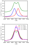 |
Fig. 3. NGC 4748. Upper panel: Broad Hβ component of a mock spectrum shifted redwards (red line) and bluewards (blue line) to mimic the orbital velocity of an equal-mass MBHB with orbital period τorb = 50 yr. The green line shows the composite line associated to the mock MBHB. Lower panel: Composite broad Hβ lines for mock MBHBs with τorb = 50, 100, 300, and 1000 yr (green, red, blue, and magenta lines, respectively). The Doppler shifts are evaluated assuming an edge-on circular binary with the MBH velocities perfectly aligned with the line of sight. |
We then apply FUVT to these new sets of mock spectra. The resulting profile of  as a function of
  for the four mock MBHBs constructed starting from NGC 4748 are shown in Fig. 4.
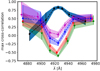 |
Fig. 4. Same as Fig. 1, but for the four mock MBHBs obtained from NGC 4748. The green, red, cyan, and magenta points with uncertainties are for binaries with τ orb = 50, 100, 300, and 1000 yr, respectively. The original values and uncertainties of NGC 4748 are shown in blue for comparison. “Solid” binaries are shown with dashed lines, while dotted lines show shorter-period binaries. |
The four mock binaries show clearly different  profiles with respect to the single MBH case; they tend to have significantly smaller values of
  than the single MBH cases close to the bulk of the broad line: the shorter the period, the larger the frequency separation between the binary component contributions, and the lower the
  . The highest values of the mock MBHB cross-correlation are instead found close to the line wings, where a correlation might be found due to the low signal-to-noise ratio of one of the two sides of the line. The anti-correlation observable for central values of
  is due to the shape of the broad Hβ light curve, which features a single peak appearing after a dimmer state (see Fig. 2 and the following discussion in this section). Such an anti-correlation should not be considered a solid feature associated with binarity; indeed, it is not observed in some of the other systems. We note that even the mock binary with a 1000 yr period shows a clear minimum in the
  profile, with the two parts of the line being almost completely uncorrelated, regardless of the relatively small velocity shift between the two components associated with the two MBHs. In this case, the relative velocity between the two MBHs is ≈500 km s−1 (equivalently, the shift of one of the peaks with respect to the centroid is ≈250 km s−1), and the FWHM of the Hβ line is ≈2000 km s−1 (σ ≈ 1000 km s−1) in the mean spectrum for NGC 4748. If we consider the varying component only, looking at the RMS spectrum for the same system, we get FWHM ≈ 1200 km s−1 (σ ≈ 650 km s−1)8. While the velocity shift is smaller than the FWHM, our test still manages to identify the mock as a binary.
More generally, four other sets of mock binaries based on other observed AGN show trends that are qualitatively similar to the one shown in Fig. 4; three sets have values of  that can be higher or lower than that of the single MBH case, depending on the choice of orbital period; and one set has lower
  compared to the corresponding single MBH, which nevertheless remains relatively high, up to ≈0.75. An example mock binary for each of the last two classes is shown in Fig. 59. The occurrence of different behaviours is not surprising, because the actual profile of
  depends mostly on the shape of the original Hβ light curve used to generate the mock binary. If the original Hβ light curve displays a single peak and single drop with similar duration, the corresponding binaries will tend towards anti-correlation when two-close-to-equal-flux parts of the composite Hβ are considered. If the original Hβ light curve instead shows a more rapid variability, the shift of half of the duration of the observations may result in close to zero correlation. If instead the Hβ light curve, for example, shows two peaks and two troughs, both equally spaced and of similar duration, the time shift will not significantly reduce the maximum cross-correlation. We stress that such a variety of behaviours is due to the limited timescale of the spectroscopic monitoring campaigns. In principle, in the binary scenario, a campaign of arbitrary timescale would have a collection of BEL profiles (one per pointing) that are contributed from the two completely uncorrelated components (1 and 2) associated to the two MBHs. In this case, when cross-correlating the blue and red parts of the total BEL, the cross terms in the cross-correlation would be equal to zero10. The cross correlation between the two sides of the BEL would then read:
 (5)
(5)
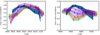 |
Fig. 5. Same as Fig. 4 but for NGC 5548 and the associated mock binaries (left panel) and for Mrk 202 (right panel). The case on the left represents a class of objects in which the max cross-correlation in the bulk of the broad line can be higher or lower than that of the single MBH depending on the assumed period. The right panel shows the only case in which the single MBH has a value of |

where σ(x) is the standard deviation of the x quantity. In the simplifying case, in which the time delay maximising the cross-correlation is the same for the two components, as is the case for our mock binaries, we obtain
 (6)
(6)
From Eqs. (5) and (6), we can derive some interesting trends and limits: when the shifts of the two components (due to the velocity of the two MBHs along the line of side) tend to zero, and the line is split approximately in half, the denominator of the σ ratios tends to 2 σ(r1) σ(b1)≈2 σ(r2) σ(b2), and the cross-correlation in Eqs. (5) and (6) tends to the arithmetic average of the cross-correlation between the blue and red parts of the two single components. If these cross-correlations are strong (as expected for a single MBH–BLR system; see Sect. 3), the total cross-correlation will be equally strong, as expected when there is zero velocity shift between the two components. On the other hand, the maximum cross-correlation in Eq. (6) will become lower and lower (while remaining positive) as the two components 1 and 2 become more shifted from the reference frame of the galaxy and contribute more asymmetrically to the red and blue parts of the whole line. Unfortunately, in many cases (such as those considered in this paper), the length of the RM campaigns will not be sufficient to ensure that the two components are completely uncorrelated, leading to the variety of outcomes mentioned above. The dependence of the profile of  for binaries on the specific realisation of the variability observed during the RM campaign has important implications for the identification of the studied systems as MBHBs. In following section, we further discuss this point.
In principle, with a sufficiently large population of single MBHs studied with RM in order to constrain the distribution of  in the line bulk (i.e. measured for one of the three central
  ), we could translate the values of
  of our mock binaries into a probability of not belonging to the “standard” population. To date, this distribution is largely unconstrained. As an example, in Fig. 6 we show the distributions of
  for the observed single MBHs discussed in Sect. 3 (blue histogram) and the mock binaries (red histograms). The two distributions are clearly different. Starting from the observed
  for the nine AGNs, we construct a model of the
  distribution for “typical” single MBH, which we then use to infer the probability that mocks belong to the single MBH population. Our model is based on the assumption that (i) the population of single MBHs has a well-defined value of
  , and that (ii) the red and blue parts of the Hβ flux data follow a bivariate Gaussian distribution, with the aforementioned, unknown correlation coefficient
  . The latter allows us to exploit the analytical form of the sampling distribution of the
  derived by Fisher (1928) given a set of observed
  . We infer a posterior distribution for
  using a nested sampling algorithm, which we use as the model for the expected distribution of measured
  for single MBHs. The cumulative probability of observing a given value of
  (again restricting our search to the bulk of the BELs) is shown as a black curve in Fig. 6. The vertical blue and red ticks highlight the values of
  measured for all the observed single and mock binaries in the bulk of the BEL. Mocks with lower values of
  have lower probabilities, with 24 (out of 36) mocks having a probability of < 10−3. The values of
  and of the associated probabilities are reported in Table 111.
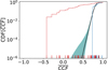 |
Fig. 6. Normalised cumulative distribution of the observed single MBHs (blue histogram) and of our mock MBHBs (red histrogram). The solid black line shows the median cumulative probability that a system will have a |


Values of  and the associated probability of belonging to the distribution of single MBHs for single and (mock) binary MBH.
5. Discussion
We present a novel method (FUVT) to search for MBHBs and to test the binary hypothesis in already identified MBHB candidates. The method is tailored to seek large separation binaries, when the two MBHs can retain their own BLR, with orbital periods that can be ≳50 yr. FUVT assumes that the two MBHs are at sufficiently large distances to ensure that the short-term variability of the two BLRs is uncorrelated. A simple correlation test between the long- and short-wavelength parts of BELs can therefore identify binaries if the maximum cross-correlation (once the BELs have been split into two comparable flux components) is sufficiently small compared to the high level of correlation expected and observed for single MBHs.
As opposed to the already proposed SPT, which requires follow-up campaigns with a minimum duration of ∼τorb in order to track the expected evolution of the orbital velocity of one active component of the binary, FUVT works on significantly shorter observational campaigns. The expected timescales of the test are from weeks to a few years in the worst-case scenario, provided that a sufficiently frequent time coverage (typical of RM studies) of the candidate spectra is achieved.
In addition to the obvious advantage of its short duration, FUVT has a number of specific advantages and disadvantages with respect to SPT, making the two procedures complementary:
-
FUVT performs best when the two MBHs in the binary have similar BEL luminosities, on average. According to theoretical studies (e.g. Roedig et al. 2012; Duffell et al. 2020, and references therein), secondary MBHs are expected to experience higher accretion rates, making FUVT particularly relevant either for systems of close to equal mass (and equal Eddington ratio) or for systems in which the secondary luminosity is close to its Eddington limit. If the flux coming from one of the two BLRs is too small compared to the other, FUVT could fail in distinguishing the subdominant contribution from the observational noise.
-
If however the two MBHs contribute similarly to the BELs, the previously proposed tests (and SPT in particular) could miss real binaries, because at large separations, double-peaked profiles are not always detectable (see e.g. Fig. 3) or could be misinterpreted as the indication of a disc-like BLR, as in the standard interpretation for the broad double-peaked emitters (e.g. Eracleous & Halpern 1994). Even if a binary is selected as a candidate at a time when one MBH was significantly brighter than the other, SPT could fail in observing a long-term frequency shift consistent with the orbital evolution of a binary if the other component undergoes a sizable rebrightening, changing the shape (and centroid) of the line. Such an evolution could result in the erroneous dismissal of real binaries if only SPT is performed, while the binary nature of the system would be easily identifiable by FUVT.
-
As discussed in Sect. 4, the stochastic nature of the short-term variability of each MBH accretion disc can occasionally result in strong cross-correlations even if the observed AGN hosts a real MBHB. If FUVT is applied to large spectroscopic catalogues to identify new MBHB candidates, a fraction of the MBHBs in the data are expected not to be missed. It is difficult to estimate a solid missed detection fraction because of the small number of single MBHs that we use to characterize the “control sample”. However, taking the probabilities we estimated (with a priori assumptions on the shape of p(CC), which will be verified when enough data become available), and assuming a “missed” alarm threshold of p ≥ 0.01 (corresponding to CC ≥ 0.70), we get 10 systems out of 36 (≈28% of missed binaries), including binaries with a period shorter than 300 yr, or 9 out of 18 when considering only larger “solid” binaries (see discussion in Sect. 2). Such shortcomings can be circumvented when FUVT is applied to data taken from a significantly longer campaign with equally frequent observations, motivated for example by the objective to independently identify a source as a promising MBHB candidate. In this case, if the first observational campaign finds a high correlation in the red and blue part of the BELs, the test should be considered inconclusive, and a new campaign should be performed. Only after a few campaigns (for a total of a few years, in the worst-case scenario) can the binary hypothesis be ruled out (unless a low correlation period is found, in which case the binary nature is indeed confirmed). However, we note that the missed detection fraction estimated here cannot be used to infer the statistics of the global MBHB population, because in this first method paper we are considering only the idealised edge-on and Doppler-maximising configuration for equal-mass binaries. A broader analysis of the binary parameter space, including a statistical estimate of the minimum number of observational campaigns needed to disprove the MBHB scenario with at a given confidence level, is postponed to a future study.
-
Finally, we stress that all the currently spectroscopically selected MBHB candidates have masses of ≳108 M⊙ (e.g. Tsalmantza et al. 2011; Eracleous et al. 2012), and no candidates in the 105 − 107 M⊙ range of interest for the future gravitational wave interferometer LISA have yet been identified. This might be due to a selection effect specific of the traditional spectroscopic search. Indeed, in order to be selected as MBHB candidates, the BELs are typically required to be shifted by ≳1000 km s−1 (Tsalmantza et al. 2011; Eracleous et al. 2012) with respect to the host rest frame (traced by the narrow emission lines) in order to prevent the inclusion of single MBHs with slightly asymmetric BLRs. This threshold can be higher than the maximum velocity for which the secondary of a MBHB can retain its own BLR12:
 (7)
(7)where
![Mathematical equation: $$ \begin{aligned} f(q) = q^{1/3}(1+q)\left[0.6q^{2/3}+\ln {(1+q^{1/3}})\right], \end{aligned} $$](/articles/aa/full_html/2023/12/aa46916-23/aa46916-23-eq59.gif) (8)
(8)for small secondary masses and binaries of close to equal mass, unless the Eddington ratio is small. For example, M2 = 106 M⊙ and q = 1 would require fEdd ≲ 0.01 to have a maximum secondary velocity of v2 ≈ 1000 km s−1. For such small masses and low fEdd, collecting a spectrum with a sufficiently high signal-to-noise ratio to perform the test might be prohibitively challenging. Nevertheless, FUVT could still succeed in identifying a MBHB (as it does for three mock MBHBs with periods of 1000 yr), if the random fluctuations of the two MBHs do not appear correlated by chance (see the discussion above).
As a final note, we stress that the procedure we discuss could, in principle, identify false-positive MBHB if the structure of the BLR around a single MBH is sufficiently complex, with strong asymmetries, including for example long-lived spiral waves (e.g. Storchi-Bergmann et al. 2003) or hot spots (e.g. Fries et al. 2023). If a large and representative distribution of  were available for bona fide symmetric single MBHs, FUVT could identify subpopulations of outliers. Their deviation from a reference
  distribution would provide an estimate of the probability that such systems do not belong to the “normal” single MBH distribution (as exemplified in Sect. 4), allowing the selection of candidates to be further analysed to discriminate between the two (asymmetric single BLR and MBHB) scenarios. We speculate that the inclusion of the information on the cross-correlation of the two (blue and red) parts of the BELs with the observed continuum could inform us about the most plausible scenario. A study quantifying false positives, that is, AGN with single asymmetric BELs, and the development of tests to identify them are ongoing. Nevertheless, we believe that currently the most limiting factor is the paucity of systems for which RM studies have been performed. Indeed, in order to estimate the probability that our mock MBHBs are outliers of the single MBH distribution, in Sect. 4 we have to assume an a priori
  distribution for single MBHs, as nine measurements are barely enough to characterise the distribution. However, the situation will improve significantly thanks to future large RM campaigns (e.g. the black hole mapper program of the SDSS-V, Almeida et al. 2023), adding approximately 1000 systems to the current sample, allowing far better determination of the distribution of
  for single MBHs. With a large enough sample, one could even begin to identify subpopulations within the single MBH class, ultimately leading to a more accurate identification of binary MBHs candidates. An alternative improvement could be achieved with a dedicated RM campaign on double-peaked emitters13. Such a study could provide an additional test as to the nature of individual double-peaked emitters (see also Eracleous et al. 1997; Liu et al. 2016 for different tests) and, even if all the systems prove to be single MBHs with disk-like BELs (e.g. Eracleous & Halpern 1994), could serve as a comparison for future candidates.
A boxy profile is not an unequivocal signature of a binary. Indeed, some of the observed AGN discussed in Sect. 3 have boxy profiles; see e.g. the mean spectra in Bentz et al. (2009a).
Although our procedure is slightly different from that used in Bentz et al. (2009a), we recover the same fluxes (within uncertainties) from the whole broad Hβ for every pointing of every AGN.
The number of  used to spit the BEL is indeed somewhat arbitrary. We used eight as it is the maximum number of bins used in Bentz et al. (2009a) for 2D RM of the nine single MBHs, which was chosen in order to keep a sufficiently high signal-to-noise ratio in each frequency bin.
We modified the public version to also output the uncertainties on the cross-correlation.
We stress again that  refers to the maximum CCF over all the possible
  while
while  refers to the maximum CCF for a specific
  .
.
The profiles of  for all the other single MBHs as well as for all the mock binaries discussed in the following section are available at https://astro.fisica.unimib.it/spectroscopical-search-of-massive-black-hole-binaries/
We acknowledge that we could also enforce not-causally related light curves by using two different AGN. Unfortunately, due to the limited number of single MBHs, only two pairs have a small enough redshift difference to be interpreted as a relative velocity between two loosely bound MBHs. We defer an investigation of “heterogeneous” mock binaries to a future study.
All the values of σ and FWHM obtained from our analysis are consistent with those presented in Bentz et al. (2009a).
The profiles of  for all the other single MBHs and mock binaries are available at https://astro.fisica.unimib.it/spectroscopical-search-of-massive-black-hole-binaries/
I.e. the red part of component 1 (r1) would have a zero cross-correlation with the blue part of component 2 (b2).
We stress that the somewhat low probability values for two of the single MBHs (Mrk 142 and NGC 5548) should be considered with caution, because the functional form of the probability distribution was decided a priori for this exercise.
The two approaches do not necessarily require independent observational campaigns, as double-peaked components might be frequent (or even ubiquitous) in type I AGN (Storchi-Bergmann et al. 2017).
Acknowledgments
The authors thank G. De Rosa and M. Bentz for their help with the RM datasets, and M. Eracleous, Z. Haiman and D. J. D’Orazio for their useful comments and suggestions. M.D. acknowledges funding from MIUR under the grant PRIN 2017-MB8AEZ, and financial support from ICSC – Centro Nazionale di Ricerca in High Performance Computing, Big Data and Quantum Computing, funded by European Union – NextGenerationEU. R.B. acknowledges support through the Italian Space Agency grant Phase A activity for LISA mission, Agreement n. 2017-29-H.0, CUP F62F17000290005.
References
- Ackermann, M., Ajello, M., Albert, A., et al. 2015, ApJ, 813, L41 [NASA ADS] [CrossRef] [Google Scholar]
- Almeida, A., Anderson, S. F., Argudo-Fernández, M., et al. 2023, ApJS, 267, 44 [NASA ADS] [CrossRef] [Google Scholar]
- Amaro-Seoane, P., Audley, H., Babak, S., et al. 2017, arXiv e-prints [arXiv:1702.00786] [Google Scholar]
- Amaro-Seoane, P., Andrews, J., Arca Sedda, M., et al. 2023, Liv. Rev. Rel., 26, 2 [NASA ADS] [CrossRef] [Google Scholar]
- Begelman, M. C., Blandford, R. D., & Rees, M. J. 1980, Nature, 287, 307 [Google Scholar]
- Bentz, M. C., Walsh, J. L., Barth, A. J., et al. 2009a, ApJ, 705, 199 [NASA ADS] [CrossRef] [Google Scholar]
- Bentz, M. C., Peterson, B. M., Netzer, H., Pogge, R. W., & Vestergaard, M. 2009b, ApJ, 697, 160 [Google Scholar]
- Blandford, R. D., & McKee, C. F. 1982, ApJ, 255, 419 [Google Scholar]
- Bortolas, E., Capelo, P. R., Zana, T., et al. 2020, MNRAS, 498, 3601 [Google Scholar]
- Bortolas, E., Bonetti, M., Dotti, M., et al. 2022, MNRAS, 512, 3365 [NASA ADS] [CrossRef] [Google Scholar]
- Burke-Spolaor, S. 2011, MNRAS, 410, 2113 [Google Scholar]
- Charisi, M., Bartos, I., Haiman, Z., et al. 2016, MNRAS, 463, 2145 [Google Scholar]
- Chen, Y.-C., Liu, X., Liao, W.-T., et al. 2020, MNRAS, 499, 2245 [Google Scholar]
- Davelaar, J., & Haiman, Z. 2022a, Phys. Rev. Lett., 128, 191101 [NASA ADS] [CrossRef] [Google Scholar]
- Davelaar, J., & Haiman, Z. 2022b, Phys. Rev. D, 105, 103010 [NASA ADS] [CrossRef] [Google Scholar]
- Decarli, R., Dotti, M., Fumagalli, M., et al. 2013, MNRAS, 433, 1492 [Google Scholar]
- del Valle, L., Escala, A., Maureira-Fredes, C., et al. 2015, ApJ, 811, 59 [NASA ADS] [CrossRef] [Google Scholar]
- D’Orazio, D. J., & Di Stefano, R. 2018, MNRAS, 474, 2975 [CrossRef] [Google Scholar]
- D’Orazio, D. J., Haiman, Z., & Schiminovich, D. 2015, Nature, 525, 351 [Google Scholar]
- Dotti, M., Bonetti, M., D’Orazio, D. J., Haiman, Z., & Ho, L. C. 2022, MNRAS, 509, 212 [Google Scholar]
- Dotti, M., Bonetti, M., Rigamonti, F., et al. 2023, MNRAS, 518, 4172 [Google Scholar]
- Duffell, P. C., D’Orazio, D., Derdzinski, A., et al. 2020, ApJ, 901, 25 [NASA ADS] [CrossRef] [Google Scholar]
- Eggleton, P. P. 1983, ApJ, 268, 368 [Google Scholar]
- Eracleous, M., & Halpern, J. P. 1994, ApJS, 90, 1 [NASA ADS] [CrossRef] [Google Scholar]
- Eracleous, M., Halpern, J. P., Gilbert, M. A., Newman, J. A., & Filippenko, A. V. 1997, ApJ, 490, 216 [NASA ADS] [CrossRef] [Google Scholar]
- Eracleous, M., Boroson, T. A., Halpern, J. P., & Liu, J. 2012, ApJS, 201, 23 [Google Scholar]
- Fiacconi, D., Mayer, L., Roškar, R., & Colpi, M. 2013, ApJ, 777, L14 [NASA ADS] [CrossRef] [Google Scholar]
- Fisher, R. A. 1928, Proc. R. Soc. Lond. Ser. A-Contain. Pap. Math. Phys. Character, 121, 654 [Google Scholar]
- Fries, L. B., Trump, J. R., Davis, M. C., et al. 2023, ApJ, 948, 5 [NASA ADS] [CrossRef] [Google Scholar]
- Gaskell, C. M. 1996, Jets from Stars and Galactic Nuclei, 471, 165 [NASA ADS] [CrossRef] [Google Scholar]
- Graham, M. J., Djorgovski, S. G., Stern, D., et al. 2015, MNRAS, 453, 1562 [Google Scholar]
- Hayasaki, K., Mineshige, S., & Ho, L. C. 2008, ApJ, 682, 1134 [NASA ADS] [CrossRef] [Google Scholar]
- Ju, W., Greene, J. E., Rafikov, R. R., Bickerton, S. J., & Badenes, C. 2013, ApJ, 777, 44 [Google Scholar]
- Kaspi, S., Smith, P. S., Netzer, H., et al. 2000, ApJ, 533, 631 [Google Scholar]
- Li, Y.-R., Wang, J.-M., Ho, L. C., et al. 2016, ApJ, 822, 4 [NASA ADS] [CrossRef] [Google Scholar]
- Li, Y.-R., Wang, J.-M., Zhang, Z.-X., et al. 2019, ApJS, 241, 33 [Google Scholar]
- Liu, J., Eracleous, M., & Halpern, J. P. 2016, ApJ, 817, 42 [NASA ADS] [CrossRef] [Google Scholar]
- Liu, T., Gezari, S., Ayers, M., et al. 2019, ApJ, 884, 36 [Google Scholar]
- Montuori, C., Dotti, M., Colpi, M., Decarli, R., & Haardt, F. 2011, MNRAS, 412, 26 [NASA ADS] [CrossRef] [Google Scholar]
- Nguyen, K., Bogdanović, T., Runnoe, J. C., et al. 2019, ApJ, 870, 16 [Google Scholar]
- Peterson, B. M., Wanders, I., Horne, K., et al. 1998, PASP, 110, 660 [Google Scholar]
- Peterson, B. M., Ferrarese, L., Gilbert, K. M., et al. 2004, ApJ, 613, 682 [Google Scholar]
- Rodriguez, C., Taylor, G. B., Zavala, R. T., Pihlström, Y. M., & Peck, A. B. 2009, ApJ, 697, 37 [NASA ADS] [CrossRef] [Google Scholar]
- Roedig, C., Sesana, A., Dotti, M., et al. 2012, A&A, 545, A127 [NASA ADS] [CrossRef] [EDP Sciences] [Google Scholar]
- Runnoe, J. C., Eracleous, M., Mathes, G., et al. 2015, ApJS, 221, 7 [NASA ADS] [CrossRef] [Google Scholar]
- Runnoe, J. C., Eracleous, M., Pennell, A., et al. 2017, MNRAS, 468, 1683 [Google Scholar]
- Sandrinelli, A., Covino, S., Dotti, M., & Treves, A. 2016, AJ, 151, 54 [NASA ADS] [CrossRef] [Google Scholar]
- Sandrinelli, A., Covino, S., Treves, A., et al. 2018, A&A, 615, A118 [NASA ADS] [CrossRef] [EDP Sciences] [Google Scholar]
- Severgnini, P., Cicone, C., Della Ceca, R., et al. 2018, MNRAS, 479, 3804 [Google Scholar]
- Shen, Y., & Loeb, A. 2010, ApJ, 725, 249 [NASA ADS] [CrossRef] [Google Scholar]
- Shen, Y., Liu, X., Loeb, A., & Tremaine, S. 2013, ApJ, 775, 49 [Google Scholar]
- Songsheng, Y.-Y., Xiao, M., Wang, J.-M., & Ho, L. C. 2020, ApJS, 247, 3 [NASA ADS] [CrossRef] [Google Scholar]
- Souza Lima, R., Mayer, L., Capelo, P. R., & Bellovary, J. M. 2017, ApJ, 838, 13 [NASA ADS] [CrossRef] [Google Scholar]
- Storchi-Bergmann, T., Nemmen da Silva, R., Eracleous, M., et al. 2003, ApJ, 598, 956 [NASA ADS] [CrossRef] [Google Scholar]
- Storchi-Bergmann, T., Schimoia, J. S., Peterson, B. M., et al. 2017, ApJ, 835, 236 [Google Scholar]
- Sun, M., Grier, C. J., & Peterson, B. M. 2018, Astrophysics Source Code Library [record ascl:1805.032] [Google Scholar]
- Tamburello, V., Capelo, P. R., Mayer, L., Bellovary, J. M., & Wadsley, J. W. 2017, MNRAS, 464, 2952 [CrossRef] [Google Scholar]
- Tsalmantza, P., Decarli, R., Dotti, M., & Hogg, D. W. 2011, ApJ, 738, 20 [Google Scholar]
- Valtonen, M. J., Lehto, H. J., Nilsson, K., et al. 2008, Nature, 452, 851 [Google Scholar]
- Verbiest, J. P. W., Lentati, L., Hobbs, G., et al. 2016, MNRAS, 458, 1267 [Google Scholar]
- Wang, L., Greene, J. E., Ju, W., et al. 2017, ApJ, 834, 129 [Google Scholar]
- Wang, J.-M., Songsheng, Y.-Y., Li, Y.-R., & Yu, Z. 2018, ApJ, 862, 171 [NASA ADS] [CrossRef] [Google Scholar]
All Tables
Values of and the associated probability of belonging to the distribution of single MBHs for single and (mock) binary MBH.
All Figures
|
Fig. 1. NGC 4748: Maximum value of the cross correlation between the blue and red parts of the broad Hβ line as a function of the dividing wavelength |
| In the text | |
|
Fig. 2. NGC 4748: Original light curve of the entire Hβ line (blue line), the same light curve shifted by half of the observational period (with periodic boundary conditions, red line), and the sum of the two (rigidly shifted towards lower fluxes for visualisation purposes, green line), mimicking a MBHB whose components evolve independently on short timescales. |
| In the text | |
|
Fig. 3. NGC 4748. Upper panel: Broad Hβ component of a mock spectrum shifted redwards (red line) and bluewards (blue line) to mimic the orbital velocity of an equal-mass MBHB with orbital period τorb = 50 yr. The green line shows the composite line associated to the mock MBHB. Lower panel: Composite broad Hβ lines for mock MBHBs with τorb = 50, 100, 300, and 1000 yr (green, red, blue, and magenta lines, respectively). The Doppler shifts are evaluated assuming an edge-on circular binary with the MBH velocities perfectly aligned with the line of sight. |
| In the text | |
|
Fig. 4. Same as Fig. 1, but for the four mock MBHBs obtained from NGC 4748. The green, red, cyan, and magenta points with uncertainties are for binaries with τ orb = 50, 100, 300, and 1000 yr, respectively. The original values and uncertainties of NGC 4748 are shown in blue for comparison. “Solid” binaries are shown with dashed lines, while dotted lines show shorter-period binaries. |
| In the text | |
|
Fig. 5. Same as Fig. 4 but for NGC 5548 and the associated mock binaries (left panel) and for Mrk 202 (right panel). The case on the left represents a class of objects in which the max cross-correlation in the bulk of the broad line can be higher or lower than that of the single MBH depending on the assumed period. The right panel shows the only case in which the single MBH has a value of |
| In the text | |
|
Fig. 6. Normalised cumulative distribution of the observed single MBHs (blue histogram) and of our mock MBHBs (red histrogram). The solid black line shows the median cumulative probability that a system will have a |
| In the text | |
Current usage metrics show cumulative count of Article Views (full-text article views including HTML views, PDF and ePub downloads, according to the available data) and Abstracts Views on Vision4Press platform.
Data correspond to usage on the plateform after 2015. The current usage metrics is available 48-96 hours after online publication and is updated daily on week days.
Initial download of the metrics may take a while.