| Issue |
A&A
Volume 679, November 2023
|
|
|---|---|---|
| Article Number | A63 | |
| Number of page(s) | 9 | |
| Section | Numerical methods and codes | |
| DOI | https://doi.org/10.1051/0004-6361/202346998 | |
| Published online | 08 November 2023 | |
An improved spectral extraction method for JWST/NIRSpec fixed slit observations
1
Université de Lyon, Université Lyon 1, ENS de Lyon, CNRS, Centre de Recherche Astrophysique de Lyon, UMR5574,
69230
Saint-Genis-Laval, France
e-mail: This email address is being protected from spambots. You need JavaScript enabled to view it.
2
Université de Lyon, Université Lyon 1, ENS de Lyon, CNRS, Laboratoire de Géologie-Terre, Planètes, Environnement, UMR5276,
69622
Villeurbanne Cedex, France
3
Laboratoire de Recherche de l’EPITA, EPITA,
94270
Le Kremlin-Bicêtre, France
4
Space Telescope Science Institute,
Baltimore, MD
21218, Maryland, USA
5
European Space Agency, ESAC,
28692
Villafranca del Castillo,
Madrid, Spain
Received:
24
May
2023
Accepted:
25
September
2023
Abstract
The James Webb Space Telescope is performing beyond our expectations. Its Near Infrared Spectrograph (NIRSpec) provides versatile spectroscopic capabilities in the 0.6–5.3 µm wavelength range, where a new window is opening for studying Trans-Neptunian objects in particular. We propose a spectral extraction method for NIRSpec fixed slit observations, with the aim of meeting the superior performance on the instrument with the most advanced data processing. We applied this method on the fixed slit dataset of the guaranteed-time observation program 1231, which targets Plutino 2003 AZ84. We compared the spectra we extracted with those from the calibration pipeline.
Key words: methods: numerical / techniques: image processing / Kuiper belt objects: individual: 2003 AZ84 / techniques: imaging spectroscopy
© The Authors 2023
 Open Access article, published by EDP Sciences, under the terms of the Creative Commons Attribution License (https://creativecommons.org/licenses/by/4.0), which permits unrestricted use, distribution, and reproduction in any medium, provided the original work is properly cited.
This article is published in open access under the Subscribe to Open model. This email address is being protected from spambots. You need JavaScript enabled to view it. to support open access publication.
1 Introduction
With its unprecedented sensitivity, the James Webb Space Telescope (JWST) is expected to enable great advances in many fields of astrophysics. On board JWST, the Near Infrared Spectrograph (NIRSpec) provides spectroscopic capabilities in the 0.6–5.3 µm wavelength range with different observing modes. This provides a great versatility for observations of any type of target, from Solar System objects to very distant galaxies. Of particular interest to this work, fixed flits (FS) allow high-sensitivity observations of very faint single targets. A full description of the instrument from its design to its performance on the sky is given in several dedicated publications (Jakobsen et al. 2022; Ferruit et al. 2022; Böker et al. 2022, 2023; Birkmann et al. 2022). Available observing modes include multi-object spectroscopy with adjustable microshutter arrays (MSAS), an integral field unit (IFU) that provides simultaneous spatial and spectral information, and FSs of various sizes (0.2″, 0.4″, and 1.6″ in width). Of particular interest to this work, the FSs allow higher-sensitivity observations of faint point sources than the IFU, at the cost of two-dimensional (2D) spatial information. The optical performance of the telescope is significantly better than expected, which most benefits the performance of NIRSpec (e.g., Feinberg et al. 2022). Therefore, the processing of data acquired with JWST/NIRSpec FS observations must match the superior performance of this instrument in order to ensure the best scientific outcomes.
NIRSpec data can be processed by the JWST Science Calibration Pipeline1. The aim of this tool is to provide a quick look at the data, and constant improvement over time will eventually enable the calibration pipeline to provide scientifically valuable products. All reference files are continuously updated when new calibration data are available, so that data can be reprocessed to match the evolution in detector and throughput performance. At present, raw integrations are corrected for various detector effects such as dark subtraction, linearity correction, or cosmic ray hits. In a second stage, the parametric instrument model is used to calculate the wavelength and spatial coordinates per pixel. The instrument throughput losses are corrected for using three-component flat field reference files. At this stage, spectral extractions are also performed on a per-dither basis (a later stage combines dithers together and also performs spectral extraction, but we focused on the individual dithers as this later stage is not yet ideal). As currently implemented, default parameters in the calibration pipeline specify fixed positions and a fixed aperture width in the 2D FS data from which the 1D spectrum is to be extracted. Aperture correction factors are then interpolated onto the wavelength grid of the 1D spectrum and are used to correct for the finite aperture size. Target acquisition is typically used to place the source at an expected position within the slit, so that the fixed positions are expected to be accurate to the subpixel level. The use of standard extraction (i.e., an extraction aperture with uniform weights in the along-slit direction) leads to increased noise, however, especially at shorter wavelengths.
With this work, we aim to improve the signal-to-noise ratio (S/N) in the extracted spectra by accounting for the shape of the point spread function (PSF) and the multiple dithering using an inverse approach. We wish to contribute with this to the optimal analysis of JWST/NIRSpec FS data. We adapted the EXOSPECO method (Thé et al. 2022, 2023), which was developed to extract spectra from slit data, to take the distinct diffraction limitations of NIRSpec into account, and we thus provide a spectral extraction technique that is optimized for its FS observations. We also propose a method to directly calibrate the shape of the spectrum on the detector in preprocessed data. We compare the spectra that were extracted with our method2 to the spectra extracted from the science calibration pipeline.
The optimal spectral extraction problem is not new. Horne (1986) proposed an extraction method for CCD spectroscopy on data that were cleaned from the sky contribution and were divided by the PSF profile. With this method, the extracted spectrum is a least squares solution, weighted by the data precision matrix. This work was the starting point for several other methods. For instance, Kinney et al. (1991) proposed a technique modified from Horne’s method for slit data that accounted for the actual PSF profile in the data model. This PSF profile is to be estimated prior to the extraction in both methods. A remaining issue of both techniques is that they assume that the spectra are aligned with the pixel grid, which is not the case in practice due to image distortion. A prior processing is thus required that includes pixel interpolations and is not ideal because it introduces correlations and cannot correctly cope with defective pixels.
Subsequently, Lebouteiller et al. (2009) presented a multi-exposure data model to extract the spectrum from data of the infrared spectrograph of the Spitzer Space Telescope. This method accounts for the subpixel position of PSF centers by oversampling the data and the PSF model. Then, Piskunov et al. (2021) proposed an optimal extraction method based on a regularized inverse approach for echelle spectra. This method can account for the shape of the spectrum by assuming that the spectrum that is to be extracted is oversampled in the data model. Both of these later methods additionally jointly estimate the PSF profile for each row of the detector. Finally, Thé et al. (2022, 2023) proposed EXOSPECO, an algorithm based on a regularized inverse approach, for the characterization of exoplanets in long slit spectroscopy. EXOSPECO is applicable for multiframe extraction, and its direct model accounts for chromatic PSF and for spatio-spectral dispersion laws. This method has the advantage of being flexible, and it can therefore easily be adapted to the JWST/NIRSpec preprocessed FS data that have not been corrected for distortion (and thus are not resampled).
2 Our test dataset: JWST/NIRSpec FS observations of Plutino 2003 AZ84
2.1 Early JWST observations of TNOs
Trans-Neptunian objects (TNOs) are among the prime targets of JWST/NIRSpec. Because of their small size, low surface albedo, and large heliocentric distance, most TNOs are too faint for ground-based spectroscopic facilities. As a result, near-infrared spectra have been acquired over the years for only ∼80 objects (e.g., Barkume et al. 2008; Guilbert et al. 2009; Barucci et al. 2011). However, this population is an extremely valuable probe for testing our models of Solar System formation and evolution. Their composition can trace the thermal and chemical conditions of the protoplanetary disk and the outcomes of planetary migration. The diversity of their physical characteristics can inform us about their formation mechanisms and evolutionary processes that may have affected them to different degrees. The largest TNOs (or dwarf planets) have been extensively studied, but the 3–5 µm wavelength range remains the key to lift degeneracies in their surface composition. Consequently, JWST/NIRSpec has been eagerly awaited (e.g., Parker et al. 2016; Métayer et al. 2019) to increase both the quality of the observed spectra and the number of the observed objects, but also to open the 3–5 µm wavelength range, in which key chemical bonds display strong signatures (e.g., fundamental absorption bands of C-H-, N-H-, and O-H-bearing ices).
A number of guaranteed-time observation (GTO) programs, as well as a Large Program (GO 2418; Pinilla-Alonso et al., in prep.; De Prá et al. 2023), are currently targeting TNOs, with the aim of further constraining the inventory of volatile and organic species in the outer Solar System, and of understanding the physical and chemical evolution of these bodies. Among those programs, GTO 1231 is targeting the two Plutinos Orcus and 2003 AZ84. These two medium-sized TNOs, located in the 3:2 mean-motion resonance with Neptune like Pluto, appear to be similar to Charon, the largest satellite of Pluto. In addition to water ice, traces of ammonia and/or ammonia hydrates have been found in ground-based spectra of Orcus (Barucci et al. 2008; Delsanti et al. 2010; Carry et al. 2011). However, ground-based observations of 2003 AZ84 were only able to suggest that crystalline water ice may be the dominant ice species on its surface (Guilbert et al. 2009).
Plutino 2003 AZ84 was observed on November 20, 2022, UT, at a heliocentric distance of ∼44 au and a visible magnitude of ∼20, using the FS mode of NIRSpec. The S200A1 slit (0.2″), a three-dither position pattern, and the NRSIRS2RAPID readout pattern were used. We provide in Table 1 details of the instrument and observation configurations, and we show in Fig. 1 a simplified schematic of the data acquisition process of the JWST/NIRSpec FS mode.
Spectral elements used for the observation of 2003 AZ84 with the JWST/NIRSpec FS mode.
2.2 NIRSpec FS observations of 2003 AZ84
We aim to extract the spectrum z є ℝN of 2003 AZ84, a spatially unresolved target. This spectrum is sampled for N wavelength values λ,z є ℝN that are evenly distributed between λmin and λmax, that is, with a constant step size ∆λ = (λmax − λmin)/(N − 1). It is extracted from a dataset d ∈ ℝK×L. It is composed of L frames with K pixels each, where K is the product of the quantities of pixels along the spectral and spatial dimensions. The spectral and spatial behavior of the data is given by two maps:
A wavelength map λ, ∈ [λmin, λmax]K×L, such that λ,k‚ℓ is the wavelength λ for the kth pixel of the Ith frame, and
A map ρ ∈ ℝK×L, such that ρk,ℓ is the angular position ρ along the slit of each pixel k of the ℓth frame.
These maps account for the fact that because of image distortion and the nonlinear spectral dispersion law, the spectral and angular directions are neither aligned with the detector dimensions nor evenly sampled by the pixels.
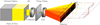 |
Fig. 1 Simplified schematics of the JWST/NIRSpec FS observation mode. The slit performs a spatial cut of the field of view. Because the target is not spatially resolved, this results in a 1D cut of the target light, diffracted by the instrument. Rays of light are then realigned in a thin beam by the collimator, in order to be properly dispersed. In our reference dataset, the dispersion of the light is made by a prism for observations with a low spectral resolving power and various gratings for observations with a medium spectral resolving power. The dispersed light is acquired by the detector with the spectral dimension in the abscissa and the spatial dimension in the ordinate. Finally, for each wavelength (λ,k,ℓ)k∈1:K,ℓ∈1:L, the spectral flux is the integral of the spatial PSF for this wavelength. |
2.3 PSF model
In the case of JWST/NIRSpec, for all λ < 3.25 µm, the full width at half-maximum (FWHM) of the PSF is smaller than a pixel and cannot be resolved. The width of the PSF is thus determined by the combination of the diffraction (scaling as the wavelength λ) and of the pixel integration. We assume that the convolution of both effects is well approximated by a Gaussian of variance α λ2 + β, with α > 0 the chromatic scaling and β > 0 the minimum width. Our PSF model is thus
 (1)
(1)
with c the target position along the slit for the considered exposure. The PSF is thus parameterized by θ = (α, β, c1,…, cL) ∈ Ω, with  and cℓ the target position in the ℓth frame. Its components are autocalibrated in our method (see Sect. 3.2). In the following, we call hθ ∈ ℝK×L the sampled PSF model for the entire dataset, that is, (hθ)k,ℓ = h(λ,k,ℓ,ρk,ℓ, α,β, cℓ).
2.4 Direct model of the data
In order to go from the spectrum sampled on λ,z ∈ ℝN to the flux sampled by the detector for each wavelength of the map λ, ∈ ℝK×L, we interpolate the model spectrum z with a given interpolation function Φ: ℝ → ℝ, which gives the following model spectrum in the data:
 (2)
(2)
with (Fk,ℓ)n = Φ( ). The interpolation function Φ we used in this work is a Catmull-Rom spline (Catmull & Rom 1974). Finally, we have the following data direct model:
 (3)
(3)
where ⊙ is the Hadamard product, and η ∈ ℝK×L is a noise vector that approximately follows a centered Gaussian law of covariance Σ. For the dataset used in this work, measurements are individually independent, and Σ is characterized by its diagonal elements  . If the kth pixel is defective, Var(dk,ℓ) = +∞. In the following, we introduce the linear operator Mθ∈ ℝKL×N such that the direct model writes hθ ⊙ (Fz) = Mθz.
3 Optimal spectral extraction method
3.1 Spectral extraction
The direct model is parameterized with four unknown parameters: the PSF parameters α and β, the target positions c in the slit, and the spectrum that is to be extracted, z. These parameters are estimated with an alternated method through minimizing the co-log-likelihood of the data with a Tikhonov (Tikhonov & Arsenin 1977) regularization,
 (4)
(4)
where ∀y ∈ ℝK,  , with W = Σ−1 the diagonal weighting matrix and D the finite difference operator such that (Dz)k = zk − zk+1. The importance of the regularization term and the tuning of its contribution in the cost function is discussed in Sect. 3.3.
For a fixed θ, the spectrum z is extracted by minimizing the cost function g(z, θ), defined in Eq. (4), with respect to z,
 (5)
(5)
which has a closed-form solution,
 (6)
(6)
3.2 Autocalibration of the PSF parameters
Once a first spectrum is extracted, the parameters α, β, and c were refined as follows. First, the PSF parameters are recalculated for a fixed c,
 (7)
(7)
Then, the centers were refined with the PSF parameters fixed to those obtained just before,
 (8)
(8)
A new spectrum is then extracted for these values using Eq. (5), and so on until the algorithm converges. The method is summarized in Algorithm 1.
The cost function (Eq. (7)) is optimized with the BOBYQA method by Powell (1994). The same applies for Eq. (8), unless the dataset is composed of only one frame. In this case, the FMΓN method by Brent (1973) is used because there is only one center to estimate. These methods optimize a given criterion using successive quadratic approximations of it. They do not require calculation of the criterion gradient.
3.3 Tuning of the regularization hyperparameter
The regularization, and thus the smoothness of the extracted spectrum, is weighted through the hyperparameter µ. Because the model Mθ is not full rank (N ≠ KL) and is ill-conditioned, the noise is amplified when the value of µ is too small (Tikhonov & Arsenin 1977; Titterington 1985). In addition, large values of µ excessively smooth the spectrum and might lead to the loss of spectral information, especially when shallow and thin absorption bands are present. Therefore, this parameter needs to be tuned optimally. The literature includes many effective methods for tuning this parameter, for instance, the generalized cross validation (GCV; Golub et al. 1979) or the Stein unbiased risk estimator (SURE; Stein 1981), which aim at minimizing an estimate of the mean square error.
We obtained the optimal value of the hyperparameter using a nonexhaustive cross validation (CV). For a given hyperparameter µ, the CV is computed as
![Mathematical equation: ${\rm{CV}} = {1 \over T}\sum\limits_{t = 1}^T {\left\| {d - {M_\theta }{\bf{z}}_\mu ^{\left[ t \right]}} \right\|_{{{\bf{W}}_{\left| {{p^{\left[ t \right]}}} \right.}}}^2} ,$](/articles/aa/full_html/2023/11/aa46998-23/aa46998-23-eq14.png) (9)
(9)
were T is the number of iterations used to compute the CV, and 𝒫[t] indicates the validation dataset, such that
![Mathematical equation: ${{\bf{W}}_{{{\left| p \right.}^{\left[ t \right]}}}} = \left\{ {\matrix{ {{{\bf{W}}_p}} & {{\rm{if}}\;p \notin {p^{\left[ t \right]}}} \cr 0 & {{\rm{else}}} \cr } } \right..$](/articles/aa/full_html/2023/11/aa46998-23/aa46998-23-eq15.png) (10)
(10)
Its complementary C𝒫[t] indicates the training dataset from whose ![Mathematical equation: ${\bf{z}}_\mu ^{\left[ t \right]}$](/articles/aa/full_html/2023/11/aa46998-23/aa46998-23-eq16.png) the spectrum is extracted for the given hyperparameter µ.
the spectrum is extracted for the given hyperparameter µ.
Nevertheless, we wished to keep control over µ, and we used multiple values of this parameter as a test of the robustness or resistance of spectral features against the regularization. Over-smoothing the spectrum with a high value of µ reduces the spectral resolution of the reconstructed spectrum. Real absorption bands remain observable, in contrast to the noise. We can thus ensure the actual presence of various absorption bands by testing their survival at a large µ, as well as by comparing spectra extracted from LR and MR exposures. This technique is in fact similar to the study of a spectrum with wavelet decomposition (e.g., Starck et al. 1997). This also motivates the study of wavelet-based regularization for future work.
4 Application to JWST/NIRSpec observations of 2003 AZ84
4.1 Data specifications and calibration
Our method was applied to 2003 AZ84 data, preprocessed (at the detector level) by the JWST calibration pipeline. The level of preprocessing we considered was 2b with the _cal extension. These preprocessed data were not yet corrected for distortion, and thus were not resampled. For comparison, the pipeline takes these _cal files, then corrects for distortion effects to produce _s2d files, such that a column in the _s2d data is associated with a single wavelength. This particular step requires interpolating along the spatial and spectral dimensions. These interpolations introduce a noise correlation and propagate the corruption by defective pixels. By default, the pipeline then extracts the spectrum by integrating the flux in a sliding window of fixed size (here with a width of 6 pixels) for each column. An additional extraction package allows the choice of an adaptive window size, but all pixels in this window remain evenly weighted. The pipeline extraction considered in this work uses the version 11.16.22 of the calibration reference data system (CRDS).
Our extraction method requires computing four maps: the data d, the weights W, the wavelength map λ, and the position map ρ. The _cal data files contain a data map, a variance map, a map of defective pixels, and the λ, map, all of which are required for application of our method. The data maps were not corrected for the thermal background contribution, which was suppressed by subtracting the mean of the other frames for each pixel from each exposure, to obtain the map d as follows:
 (11)
(11)
where the superscript bg denotes a map with the thermal background contribution. Because the data frames are mutually independent, the variance of the background-subtracted data is given by
 (12)
(12)
The resulting variance map characterizes the diagonal element of the covariance Σ, which was then combined after inversion to the map of defective pixels to create the weight matrix W.
The calibration of the ρ map on the data is one of our specific contributions to the analysis of JWST/NIRSpec FS data, and it is illustrated in Fig. 2. Taking into account the defective pixels, the calibration is done as follows:
Each column of the data map is normalized by its maximum.
Using BOBYQA, a Gaussian is fit to each column. A center and a FWHM are then retrieved for each of them (see Fig. 2a, cyan curve).
A second-order polynomial is fit to these centers (see Fig. 2a, red curve) as a function of the column number.
Finally, the ρ map is computed as
 (13)
(13)
where p is the polynomial fit in step 2, while i ∈ 1:I and j ∈ 1: J are the respective row and column indices in the map (such that M = I × J).
Figure 2b shows that the average PSF profile can be well approximated with a Gaussian model. Moreover, Fig. 2c presents some normalized cross section of the data, overlapped by the corresponding chromatic Gaussian PSF that was autocalibrated with our method. Our autocalibrated PSF matches the data well. This strengthens the use of a chromatic Gaussian model in our direct model.
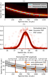 |
Fig. 2 Calibration of the distortion. (a) Fitting of the centers for the first exposure of G140M data. (b) Cloud of the normalized data values for all the wavelengths of the spectral dimension compared to the chromatic Gaussian PSF for an average wavelength. (C) Normalized cross-sections of the data and the discretized PSFs obtained after the autocalibration in Algorithm 1. |
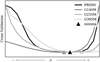 |
Fig. 3 Cross validation curves for each filter. The minima corresponding to the best value of µ for each filter are highlighted with triangles. |
4.2 Optimal extraction of the 2003 AZ84 spectrum
To proceed to the optimal extraction, we computed the cross validation with the global methods for each filter. We chose to compute the CV for T = 10, and we split randomly for each t, such that 𝒫[t] and C𝒫[t] both contained half of the data. In order to use the same splitting configurations for each value of µ, the random seed was reset to the same value before each CV computation. In the following, we call the spectrum extracted with the “best µ” the “best extraction” which is the minimum argument of the cross validation for the considered filter (see Fig. 3 for the CV curves).
4.2.1 Frame-by-frame comparison
First, we applied our extraction method on each calibrated data-frame described above. All the extracted spectra were normalized to a relative reflectance of 1 at 3 µm. This allowed a comparison of each extracted spectrum with the corresponding spectrum extracted by the pipeline, as shown in Fig. 4. The extractions performed by our method are overall less noisy. We note here that the spectra were not divided by the solar spectrum to correct for the contribution of solar light. Despite this caveat, absorption bands are clearly visible in spectra extracted by both methods, but they are more pronounced when using our method, as explained below.
4.2.2 Global inverse approach versus average spectrum
One of the strengths of our method lies in the possibility of taking multiple exposures into account to extract a single spectrum. As presented in Sect. 2.4, the L exposures are modeled as a function of this spectrum. This spectrum is then estimated using the method presented in Algorithm 1: one single spectrum is thus extracted, with an increased S/N. To compare this spectrum, we considered the average spectrum derived from the three individual spectra extracted by the pipeline. Figure 5 shows this comparison for the same hyperparameters µ as Fig. 4 and with the same normalization. We note that our method accounts for the shape of the spectrum at a subpixel level along the spatial and spectral dimensions. As a result, the spectrum quality is enhanced by this multiframe approach, with information shared between all the frames. The absorption bands are thus more evident with our method than with the pipeline, which is particularly true for the MR spectrum.
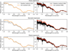 |
Fig. 4 Frame-by-frame comparison of spectra extracted from reconstructions by our method (red) and by the pipeline (black). Spectra are normalized to 1 at 3 µm. |
4.2.3 Reduction of the noise
A direct comparison between spectra extracted with our method and with the pipeline shows that the noise level is reduced and absorption bands appear more evident. We thus further explain the reasons for these effects. Because the flux is integrated column-wise by the pipeline, it cannot account for subpixel effects. Moreover, the flux is integrated in a fixed-size window of 6 pixels, but even for _s2d, the FWHMs vary with wavelength, as presented in Fig. 6. For these wavelengths, the window is too large (see Fig. 7), and because each pixel has the same weight in the integration, almost half of the integrated flux comes from the background.
Instead, our method enhances the spectral extraction in several aspects. First, we account for the varying size of the PSF. This allows an optimal extraction with the least possible contamination from noise. The regularization also helps to smooth out the noise. This is shown in Fig. 5: compared to the results of the standard pipeline, the spectra are less noisy. Second, for multiframe data, each frame is accounted for individually by the method, which can thus exploit the frame dithering to enhance the spectral quality of the extracted spectrum and its robustness against artifacts (e.g., defective pixels).
4.2.4 Influence of the regularization hyperparameter
We applied our extraction method for several values of µ in order to show its influence. The results are presented in Fig. 8. The values of µ were chosen from minus 5–6 to 0 orders of magnitude below the µ values minimizing the CV in Fig. 3. The best extractions are shown overlapping in black. The larger the value of µ, the smoother the spectrum. Consequently, we must pay special attention to small absorption bands and verify that they survive the extraction against the value of µ. As a general rule, noise is rapidly smoothed out when µ is increased, whereas actual spectral signatures remain difficult to erase. Therefore, we find that it is necessary to extract spectra for several values of µ in the case of TNOs because some ices identified on their surfaces show relatively weak, fine, and shallow bands (e.g., Pinilla-Alonso et al. in preparation). As a sanity check, a visual inspection of these multiple extractions helps to confirm that the identified absorption bands are real.
We can also observe that a fixed hyperparameter will not smooth in the same way for the short and long wavelengths. The reason is that there is less flux in the spectrum for long wavelengths than for the short ones. Hence there is more noise for long wavelengths, and a larger hyperparameter is necessary to smooth out the noise. This explains the shape and the location of the minima of the cross validation in Fig. 3.
Finally, when the MR reconstruction is oversmoothed, the extraction is coherent with LR extractions. The remaining visible bands correspond to those that are visible in the LR extraction.
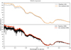 |
Fig. 5 Comparison of the spectra extracted by our method (red and orange) to the average spectra extracted from the pipeline (black and gray). Spectra are normalized to 1 at 3 µm. |
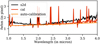 |
Fig. 6 Comparison of the FWHM approximated from _cal (red) and _s2d (black) flies. The comparison is made on PRISM second-exposure data. The FWHM obtained after autocalibration is also displayed in orange. |
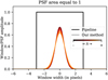 |
Fig. 7 Comparison of the pipeline window shape and the spatial PSF shape in our method (see Eq. (1)) for λ ∈ {1, 1.5, 2, 2.5, 3, 3.5) microns. |
5 Discussion and perspectives
As of today, only a few medium-sized TNOs have been characterized by spectroscopy with a quality sufficient to allow a robust interpretation of their compositions and of the processes that might have actively modified them from their primordial states. We know that the spectra of most medium-sized TNOs are dominated by water ice, but much less is known about the smaller objects (e.g., Barkume et al. 2008; Guilbert et al. 2009). PRISM observations will allow the detection of large and deep absorption bands for most TNOs. However, traces of volatile and organic species will be found through observations with medium and high resolving power. Because the FS mode of NIRSpec can reach fainter targets than the IFU (see Fig. 3 from Böker et al. 2023), the observation of medium-sized and smaller TNOs will benefit from this observing mode. Therefore, an effective spectral extraction method for FS medium and high spectral resolving power acquisition will need to be used on future data to ensure the best use of the telescope and of the exquisite instrument performance.
The JWST calibration pipeline is a great tool that is available to the whole community for extracting these spectra. It will continue to be improved over time. At present, we have identified non-ideal aspects that affect the quality of the extracted spectra (S/N and artifacts). We thus provided an alternative extraction method, to be applied on level 2b _cal data, which avoids these problems through a multiframe inverse approach, and which will be available in a public toolbox. Absorption bands are more evident with our method because the extraction is inherently less noisy and has a higher resistance against artifacts, which ultimately helps us to constrain the surface composition of this TNO.
Further improvement of our method could be performed in the future. As presented earlier, the Tikhonov regularization penalizes the difference between two values of the spectra evenly, despite the great variation in the flux between short and long wavelengths (more than a factor 10). As a result, for the same hyperparameter, a spectrum can be satisfyingly regularized for short wavelengths and over-regularized for long wavelengths. Conversely, a spectrum that is satisfyingly regularized for long wavelengths can be under-regularized for shorter wavelengths. Hence, a regularization that takes the flux variation into account should be investigated. It might also be interesting to investigate a wavelet-based penalization. Finally, we aim to improve the spectral resolution by taking the spectral blur into account in the PSF model.
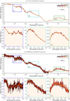 |
Fig. 8 Comparison of the smoothness of the reconstructions for different hyperparameters. |
Acknowledgements
The authors are grateful to the LABEX Lyon Institute of Origins (ANR-10-LABX-0066) for its financial support within the Plan France 2030 of the French government operated by the National Research Agency (ANR). A.G.L. received funding from the European Research Council (ERC) under the European Union’s Horizon 2020 research and innovation program (Grant Agreement No 802699). This work is based on observations made with the NASA/ESA/CSA James Webb Space Telescope. The data were obtained from the Mikulski Archive for Space Telescopes at the Space Telescope Science Institute, which is operated by the Association of Universities for Research in Astronomy, Inc., under NASA contract NAS 5-03127 for JWST. These observations are associated with program #1231. We are extremely grateful to the NIR-Spec consortium for allocating GTO time to the observation of TransNeptunian Objects.
References
- Barkume, K. M., Brown, M. E., & Schaller, E. L. 2008, AJ, 135, 55 [NASA ADS] [CrossRef] [Google Scholar]
- Barucci, M. A., Merlin, F., Guilbert, A., et al. 2008, A&A, 479, L13 [NASA ADS] [CrossRef] [EDP Sciences] [Google Scholar]
- Barucci, M. A., Alvarez-Candal, A., Merlin, F., et al. 2011, Icarus, 214, 297 [NASA ADS] [CrossRef] [Google Scholar]
- Birkmann, S. M., Ferruit, P., Giardino, G., et al. 2022, A&A, 661, A83 [NASA ADS] [CrossRef] [EDP Sciences] [Google Scholar]
- Böker, T., Arribas, S., Lützgendorf, N., et al. 2022, A&A, 661, A82 [NASA ADS] [CrossRef] [EDP Sciences] [Google Scholar]
- Böker, T., Beck, T. L., Birkmann, S. M., et al. 2023, PASP, 135, 038001 [CrossRef] [Google Scholar]
- Brent, R. 1973, Algorithms for Minimization without Derivatives (Hoboken: Prentice-Hall, Inc.) [Google Scholar]
- Carry, B., Hestroffer, D., DeMeo, F. E., et al. 2011, A&A, 534, A115 [NASA ADS] [CrossRef] [EDP Sciences] [Google Scholar]
- Catmull, E., & Rom, R. 1974, in Computer Aided Geometric Design (Amsterdam: Elsevier), 317 [CrossRef] [Google Scholar]
- De Prá, M. N., Hénault, E., Pinilla-Alonso, N., et al. 2023, Nat. Astron., submitted [Google Scholar]
- Delsanti, A., Merlin, F., Guilbert-Lepoutre, A., et al. 2010, A&A, 520, A40 [NASA ADS] [CrossRef] [EDP Sciences] [Google Scholar]
- Feinberg, L. D., Wolf, E., Acton, S., et al. 2022, SPIE Conf. Ser., 12180, 121800T [NASA ADS] [Google Scholar]
- Ferruit, P., Jakobsen, P., Giardino, G., et al. 2022, A&A, 661, A81 [NASA ADS] [CrossRef] [EDP Sciences] [Google Scholar]
- Golub, G. H., Heath, M., & Wahba, G. 1979, Technometrics, 21, 215 [Google Scholar]
- Guilbert, A., Alvarez-Candal, A., Merlin, F., et al. 2009, Icarus, 201, 272 [NASA ADS] [CrossRef] [Google Scholar]
- Horne, K. 1986, PASP, 98, 609 [Google Scholar]
- Jakobsen, P., Ferruit, P., Alves de Oliveira, C., et al. 2022, A&A, 661, A80 [NASA ADS] [CrossRef] [EDP Sciences] [Google Scholar]
- Kinney, A., Bohlin, R., & Neill, J. 1991, PASP, 103, 694 [NASA ADS] [CrossRef] [Google Scholar]
- Lebouteiller, V., Bernard-Salas, J., Sloan, G., & Barry, D. 2009, PASP, 122, 231 [Google Scholar]
- Métayer, R., Guilbert-Lepoutre, A., Ferruit, P., et al. 2019, Front. Astron. Space Sci., 6, 8 [CrossRef] [Google Scholar]
- Parker, A., Pinilla-Alonso, N., Santos-Sanz, P., et al. 2016, PASP, 128, 018010 [NASA ADS] [CrossRef] [Google Scholar]
- Piskunov, N., Wehrhahn, A., & Marquart, T. 2021, A&A, 646, A32 [NASA ADS] [CrossRef] [EDP Sciences] [Google Scholar]
- Powell, M. 1994, A Direct Search Optimization Method that Models the Objective and Constraint Functions by Linear Interpolation (Berlin: Springer) [Google Scholar]
- Starck, J.-L., Siebenmorgen, R., & Gredel, R. 1997, ApJ, 482, 1011 [NASA ADS] [CrossRef] [Google Scholar]
- Stein, C. M. 1981, Ann. Statis., 9 1135 [CrossRef] [Google Scholar]
- Thé, S., Thiébaut, É., Denis, L., Soulez, F., & Langlois, M. 2022, SPIE, 12185, 1137 [Google Scholar]
- Thé, S., Thiébaut, É., Denis, L., et al. 2023, A&A, 678, A77 [NASA ADS] [CrossRef] [EDP Sciences] [Google Scholar]
- Tikhonov, A. N., & Arsenin, V. Y. 1977, Solution of Ill-posed Problems, Scripta Series in Mathematics (Washington: Winston & Sons) [Google Scholar]
- Titterington, D. M. 1985, A&A, 144, 381 [NASA ADS] [Google Scholar]
The code of our method is available online at https://github.com/LaurenceDenneulin/AssetForJwstNirspecFs
All Tables
Spectral elements used for the observation of 2003 AZ84 with the JWST/NIRSpec FS mode.
All Figures
|
Fig. 1 Simplified schematics of the JWST/NIRSpec FS observation mode. The slit performs a spatial cut of the field of view. Because the target is not spatially resolved, this results in a 1D cut of the target light, diffracted by the instrument. Rays of light are then realigned in a thin beam by the collimator, in order to be properly dispersed. In our reference dataset, the dispersion of the light is made by a prism for observations with a low spectral resolving power and various gratings for observations with a medium spectral resolving power. The dispersed light is acquired by the detector with the spectral dimension in the abscissa and the spatial dimension in the ordinate. Finally, for each wavelength (λ,k,ℓ)k∈1:K,ℓ∈1:L, the spectral flux is the integral of the spatial PSF for this wavelength. |
| In the text | |
|
Fig. 2 Calibration of the distortion. (a) Fitting of the centers for the first exposure of G140M data. (b) Cloud of the normalized data values for all the wavelengths of the spectral dimension compared to the chromatic Gaussian PSF for an average wavelength. (C) Normalized cross-sections of the data and the discretized PSFs obtained after the autocalibration in Algorithm 1. |
| In the text | |
|
Fig. 3 Cross validation curves for each filter. The minima corresponding to the best value of µ for each filter are highlighted with triangles. |
| In the text | |
|
Fig. 4 Frame-by-frame comparison of spectra extracted from reconstructions by our method (red) and by the pipeline (black). Spectra are normalized to 1 at 3 µm. |
| In the text | |
|
Fig. 5 Comparison of the spectra extracted by our method (red and orange) to the average spectra extracted from the pipeline (black and gray). Spectra are normalized to 1 at 3 µm. |
| In the text | |
|
Fig. 6 Comparison of the FWHM approximated from _cal (red) and _s2d (black) flies. The comparison is made on PRISM second-exposure data. The FWHM obtained after autocalibration is also displayed in orange. |
| In the text | |
|
Fig. 7 Comparison of the pipeline window shape and the spatial PSF shape in our method (see Eq. (1)) for λ ∈ {1, 1.5, 2, 2.5, 3, 3.5) microns. |
| In the text | |
|
Fig. 8 Comparison of the smoothness of the reconstructions for different hyperparameters. |
| In the text | |
Current usage metrics show cumulative count of Article Views (full-text article views including HTML views, PDF and ePub downloads, according to the available data) and Abstracts Views on Vision4Press platform.
Data correspond to usage on the plateform after 2015. The current usage metrics is available 48-96 hours after online publication and is updated daily on week days.
Initial download of the metrics may take a while.