| Issue |
A&A
Volume 679, November 2023
|
|
|---|---|---|
| Article Number | A105 | |
| Number of page(s) | 13 | |
| Section | Galactic structure, stellar clusters and populations | |
| DOI | https://doi.org/10.1051/0004-6361/202346877 | |
| Published online | 20 November 2023 | |
Finding the dispersing siblings of young open clusters
Dynamical traceback simulations using Gaia DR3⋆
1
Lund Observatory, Division of Astrophysics, Department of Physics, Lund University, Box 43, 22100 Lund, Sweden
e-mail: This email address is being protected from spambots. You need JavaScript enabled to view it.
2
School of Physics & Astronomy, University of Leicester, University Road, Leicester LE1 7RH, UK
3
European Space Agency (ESA), European Space Research and Technology Centre (ESTEC), Keplerlaan 1, 2201 AZ Noordwijk, The Netherlands
Received:
11
May
2023
Accepted:
15
September
2023
Abstract
Context. Stars tend to form in clusters, but many escape their birth clusters very early. Identifying the escaped members of clusters can inform us about the dissolution of star clusters, but also about the stellar dynamics in the galaxy. Methods capable of finding escaped stars from many clusters are required to fully exploit the large amounts of data in the Gaia era.
Aims. We present a new method of identifying escaped members of nearby clusters and apply it to ten young clusters.
Methods. We assumed the escaped stars were close to the cluster in the past and performed traceback computations based on the Gaia DR3 radial velocity subsample. For each individual star, our method produces a probability estimate that it is an escaped member of a cluster, and for each cluster it also estimates the field star contamination rate of the identified fugitives.
Results. Our method is capable of finding fugitives that have escaped from their cluster in the last few ten million years. In many cases the fugitives form an elongated structure that covers a large volume.
Conclusions. The results presented here show that traceback computations using Gaia DR3 data can identify stars that have recently escaped their cluster. Our method will be even more useful when applied to future Gaia data releases that contain more radial velocity measurements.
Key words: Galaxy: kinematics and dynamics / solar neighborhood / open clusters and associations: general / stars: kinematics and dynamics / stars: formation
Full Table 4 is available at the CDS via anonymous ftp to cdsarc.cds.unistra.fr (130.79.128.5) or via https://cdsarc.cds.unistra.fr/viz-bin/cat/J/A+A/679/A105
© The Authors 2023
 Open Access article, published by EDP Sciences, under the terms of the Creative Commons Attribution License (https://creativecommons.org/licenses/by/4.0), which permits unrestricted use, distribution, and reproduction in any medium, provided the original work is properly cited.
This article is published in open access under the Subscribe to Open model. This email address is being protected from spambots. You need JavaScript enabled to view it. to support open access publication.
1. Introduction
Stars do not form in isolation: most are born in dense star-forming regions (Lada & Lada 2003). Not all stars that form together are gravitationally bound. Furthermore, the loss of mass when the leftover gas is ejected releases many more stars into the Galactic field very early in the cluster’s life. Even the clusters that are still bound after that will eventually fall apart due to the gravitational ejection of stars, close encounters with giant molecular clouds, or interactions with the Milky Way tidal field (see Krumholz & McKee 2019, for a review). Most clusters dissipate within 10 − 100 Myr, leaving many stars dispersed in the Galactic field (e.g., Lada & Lada 2003; Piskunov et al. 2006).
Identifying the escaped members of open clusters could enable further research on many topics, of which we only list a handful here. Finding exoplanet systems around young stars allows models of planet formation and migration to be refined (see, e.g., Aigrain et al. 2007), and identifying stars that have escaped young clusters can enable more such systems to be found. Kamdar et al. (2021) performed simulations of a Milky Way-like galaxy and found that it might be possible to use stellar streams from disintegrating open clusters in the Galactic disk to constrain the parameters of the Galactic bar. Dinnbier et al. (2022) have recently proposed a method of determining cluster ages based on the orientation of their tidal tails. Although their method in its current state is, strictly speaking, only applicable to clusters on circular orbits, an improved version for realistic noncircular orbits might be suitable for providing age estimates for many clusters, independent of stellar evolution models. Kroupa et al. (2022) have even suggested that the asymmetry between the number of stars in the leading and trailing tidal tails of clusters could be used as a test to compare Newtonian and Milgromian gravitation.
Stars from the same formation region can cover a large volume in position space, even if they have very similar velocities, so distinguishing escaped cluster stars from the much more numerous unrelated field stars can be like searching for a needle in a haystack. True young stellar groups are expected to be chemically homogeneous, so strong chemical tagging could contribute to the solution. However, determining detailed chemical abundances requires very high quality spectra, and the number of stars for which such spectra are available is rather low. The European Space Agency’s Gaia mission has published in its third data release (Gaia DR3; Gaia Collaboration 2021) the full six-dimensional phase space information for ∼34 million sources all over the sky. The availability of this data means that a method capable of finding cluster escapees based on kinematics rather than spectroscopy is very appealing. Even if a kinematic method is not capable of perfectly separating escaped cluster stars from field stars, it can still be valuable if it can produce a candidate list with a small enough field contamination rate, which could then be used as a starting point for further analysis (see, e.g., Bouma et al. 2021).
The convergent point method (see, e.g., Röser et al. 2019; Röser & Schilbach 2019, 2020, for recent applications) assumes that stars originating from the same cluster have similar velocities. The observed proper motion of a star can be compared with the proper motion it would have if its velocity components were replaced with the velocity components of the cluster. If the difference is too large, then the star is not considered to be associated with the cluster, but if the difference is small enough, then it might be. The convergent point method is computationally inexpensive, so it can be applied to a large number of clusters. Furthermore, stars for which radial velocity measurements are not feasible can still be included in the analysis. However, the simplest implementation of the method makes it difficult to recognize stars with velocities too similar to the cluster velocity, for which there is no reason to suspect that they were any closer to the cluster in the past than they are now.
Crundall et al. (2019) introduced a method that can provide probabilities that stars belong to associations as well as the ages of these associations. They assume associations are composed of one or more components that can be described as six-dimensional Gaussians in phase space with some specific age. The time evolution of these components in a gravitational potential can be computed, and the likelihood that observed stars belong to a component can then be used to fit its parameters. Although Crundall et al. (2019) successfully applied their method to the β Pictoris moving group, the fact that they assigned each component a specific expansion age means their method is not appropriate for studying open cluster tidal tails, which consist of stars that are escaping the cluster continuously.
Jerabkova et al. (2021) performed N-body computations in a Galactic potential to find out how the tidal tails of the open cluster Hyades should look in the phase space and then searched for stars with compatible astrometry. Their method proved to be successful at identifying stars in the Hyades tidal tails up to 800 pc away from the cluster itself. However, the N-body computations required by their method make it rather resource-intensive, so for studying a large number of clusters a simpler method is appealing.
Recently Meingast et al. (2021) searched for extended comoving stellar populations around ten nearby young open clusters. Their method involves making a hard cut in projected proper motion space followed by applying a clustering algorithm in position space. They were able to find vast stellar halos that are comoving with the clusters. Therefore, the parameter values of their clustering algorithm seem to be well justified empirically, but it is not simple to evaluate or interpret them on physical grounds. Furthermore, the use of a clustering algorithm means that they can only find the stars where the population density is relatively high.
The idea of finding escaped cluster members by looking for stars that have been close to the cluster in the past is well motivated on physical grounds. The requirement that the current position of an escapee relative to a cluster must be consistent with both its current relative velocity and escape time introduces correlations in phase space that allow us to reject many unrelated field stars that might be broadly consistent with the escapee population in every phase space coordinate individually. This idea has been utilized by Farias et al. (2020) and Schoettler et al. (2020), who both looked for stars that have escaped from the Orion Nebula Cluster. However, the Orion Nebula Cluster is young enough that both Farias et al. (2020) and Schoettler et al. (2020) ignored the Milky Way gravity entirely and assumed the stars move in straight lines with unchanging speed, so their methods are not applicable to older clusters.
In this paper we introduce a method that uses traceback computations to identify stars that have been close to the cluster in phase space in the past. Section 2 provides the details of our method and describes how it can be used to estimate individual membership probabilities for the escaped stars and also to estimate the field star contamination rate of the identified population. In Sect. 3 we outline the results of applying our method to the same ten clusters that Meingast et al. (2021) studied. We show that our method is indeed able to identify escaped cluster stars that currently cover a large volume in phase space, and we provide a brief comparison with Meingast et al. (2021). In Sect. 4 we vary some of the parameters of our analysis and show that our results are not sensitive to the exact parameter value choices we have made. Finally, Sect. 5 summarizes our conclusions and discusses the strengths and weaknesses of our method.
2. Method
2.1. General idea and definitions
We looked for stars that have escaped from a cluster by performing traceback computations and identifying the stars that have been in a small phase space volume around the cluster in the not too distant past. The search volumes we considered are spherical in both position and velocity space, with radii of rp = 15 pc and rv = 3 km s−1, respectively. In the following we call a volume with such radii around a point in phase space the “neighborhood” of that point. The position space radius of our neighborhoods is quite similar to the typical tidal neighborhood of an open cluster (∼10 pc; see, e.g., Table 2 of Meingast et al. 2021), and the velocity space radius is likewise similar to the typical velocity dispersion of stars originating from the same open cluster (a couple of km s−1; see again Table 2 of Meingast et al. 2021). Values much smaller would be too restrictive and exclude even many stars still gravitationally bound to the cluster, whereas values much larger should be expected to include too many stars that have never been gravitationally bound. We provide further empirical justification for the radii we have chosen in Sect. 4.3.
We performed 100 Monte Carlo tracebacks by sampling the current phase space coordinates of the stars based on the reported Gaia uncertainties and correlations. We interpreted the fraction of tracebacks in which a star is in the cluster neighborhood at any time up to some maximum traceback time as the star’s “fugitive probability”, pf, and the fraction of traceback simulations a star starts out in a cluster’s neighborhood as the star’s “membership probability”, pm. We point out that pf ≥ pm by definition. We also defined a “probability threshold”, pmin, and used it to divide the stars into three disjoint subsets:
-
Stars with pf ≥ pm > pmin, which we call cluster “members”. These are presently inside the cluster neighborhood or very close to it, which can be seen even without any traceback computations.
-
Stars with pf > pmin ≥ pm, which we call “fugitives”. These are not current members, but the traceback computations reveal them to have been in the cluster neighborhood in the past with a large enough probability to be of interest.
-
Stars with pmin ≥ pf ≥ pm, which we consider to be unrelated to the cluster.
We found it useful enough for our purposes to adopt the value pmin = 0.1, but a higher or a lower value could be chosen to increase the purity or the completeness of the sample, respectively. It is convenient that the probability threshold could be adjusted without having to perform a new set of traceback computations.
Our definitions do mean that in principle some stars we label as fugitives might qualify as members if a different value of pmin were used. We show empirically in Sect. 4.2 that this is not a concern in practice.
2.2. Initial selection of stars
Traceback computations require full knowledge about the kinematics of the included stars. We are therefore naturally limited to the Gaia DR3 radial velocity data set with five-parameter astrometry. We corrected for the Gaia DR3 parallax zero-point offset using the procedure outlined by Lindegren et al. (2021) and discarded sources with corrected parallaxes smaller than 1 mas. We then converted the coordinates of the stars to galactocentric cylindrical coordinates using the parameter values listed in Table 1 and retained the sources that satisfy the conditions listed in Table 2. The number of such sources is 4 238 086.
Adopted parameters of the solar orbit.
Limits for the coordinates of the stars included in the initial traceback computation.
We remark that the standard deviation of the difference between the inverted parallax of the final sample with and without the parallax offset correction is 8.3 pc and the standard deviation of the radial velocity uncertainty is 3.4 km s−1. We can make a rough estimate that for traceback times beyond the ratio of the aforementioned values 2.4 Myr the typical uncertainty in the distance of a star caused by the uncertainty of the radial velocity is larger than the distance difference that would be caused by neglecting the parallax offset entirely. Because this timescale is much shorter than the age of even the youngest cluster in our selection, we conclude that our results are not sensitive to the details of parallax offset correction.
In our Monte Carlo tracebacks, any stars with large uncertainties in astrometry or radial velocity will have a large spread in their computed past phase space coordinates, which ensures that stars with too uncertain coordinates have low fugitive probabilities. Our choice of pmin = 0.1 is therefore implicitly applying a quality cut to the data, and we can afford to not apply any explicit conditions to the uncertainties of the astrometric parameters. Furthermore, in Sect. 4.1 we show that the dominant source of uncertainty for us is the radial velocity, so commonly used quality criteria based on Gaia astrometry, such as the renormalized unit weight error (RUWE) value, are not useful for us.
2.3. Cluster coordinates
In addition to stars our traceback simulations also include points representing the clusters themselves. We refined the initial guesses of the heliocentric Cartesian phase space coordinates of a cluster by iteratively updating them to be the medians of the coordinates of all the stars within the neighborhood of the previous guess until the cluster coordinates converged. Using median rather than the mean makes the cluster coordinates less sensitive to possible field star contamination. The nominal cluster coordinates were obtained by querying the 5 astrometric parameters and radial velocity from SIMBAD (Wenger et al. 2000) with astroquery (Ginsburg et al. 2019) for the initial guess (see Table A.1) and taking the stellar coordinates from Gaia DR3, only correcting for the global parallax zero-point offset (Lindegren et al. 2021). We Monte Carlo-sampled the uncertainty of the cluster coordinates using the same iterative procedure with each set of Monte Carlo-sampled stellar coordinates and with the nominal cluster coordinates being the initial guess.
2.4. Field star contamination
Some of the stars that have been in a cluster’s neighborhood might be unrelated field stars. We estimated the number of such interlopers by counting the number of stars in the neighborhood of a reference point. This comparison is only meaningful if the reference point is carefully chosen. Assuming that the galactic field is axisymmetric and its spatial density is symmetric with respect to the galactic midplane, we can choose a reference point that has the same field star density in its neighborhood as the cluster at all times. Let the present-day cylindrical galactocentric phase space coordinates of the cluster be (R, ϕ, z, vR, vϕ, vz; see also Fig. 1) and let  be the present-day coordinates of the reference point. The reference point should have the same galactocentric distance as the cluster at all times so that the field star density in their neighborhoods would not differ because of a galactic radial density gradient, so R′=R and
  . To avoid differences caused by the galactic vertical density gradient at all times we should choose either z′=z and
  or z′= − z and
  . Our assumption of an axisymmetric field requires us to choose
  , but allows for all values of ϕ′. However, Gaia being magnitude-limited introduces a heliocentric distance bias to the observed field star density, which restricts us to three possible reference points, with galactocentric cylindrical position space coordinates (R, ϕ, −z), (R, 360° −ϕ, z) and (R, 360° −ϕ, −z). We used as the reference point the last of the three because it is the farthest from the cluster, which minimizes the chance that there are cluster fugitives in its neighborhood. In each Monte Carlo traceback the initial coordinates of the reference point were computed from the cluster coordinates sampled for that traceback.
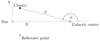 |
Fig. 1. Galactocentric cylindrical coordinates and the heliocentric Cartesian coordinates. The z (galactocentric) and Z (heliocentric) coordinates are almost perpendicular to the plane of the figure. The Sun is located at (R, ϕ, z) = (8000 pc, 180° ,14 pc), and the Galactic center is located at (X, Y, Z) = (8000 pc, 0 pc, 0 pc). |
The Sun is not exactly in the galactic midplane, so the heliocentric distance of the chosen reference point and the cluster is not exactly the same. However, the vertical offset of the Sun is small, and we ignored the distance difference this offset causes.
We required members and fugitives to have pf > pmin. Likewise, we ignored those stars for which the fraction of Monte Carlo tracebacks where they entered the reference neighborhood did not exceed pmin.
2.5. Traceback computations
We performed traceback computations using a leapfrog integrator implemented in Gala (Price-Whelan 2017). The gravitational potential we used was BovyMWPotential2014, which is the implementation of MWPotential2014 from galpy (Bovy 2015) in Gala.
We recorded the state of the computation with a timestep of 0.25 Myr, which is reasonably small compared to the timescale dictated by our choice of neighborhood radii of 15 pc/3 km s−1 ≈ 5 Myr. The maximum traceback time that should be used is more difficult to judge. On one hand, a traceback too short prevents us from finding fugitives that left their cluster early, which suggests an individual traceback time for each cluster based on its age. On the other hand, longer traceback times mean larger uncertainties of the computed phase space coordinates, which suggests a global maximum traceback time beyond which the computations are uninformative. Because it is simple to ignore the traceback results that are too far in the past, we chose a single value of 100 Myr for all the clusters, knowing that it is greater than most of the cluster ages in our sample (see Table 3). The fugitive probabilities we report, however, only consider the traceback snapshots before the cluster age estimates by Bossini et al. (2019), listed in Table 3. For the two clusters that are older than 100 Myr, we used that as the limit instead. We show in Sect. 3.2 empirically that longer traceback times are not justified with Gaia DR3 data.
Cluster ages and metallicities from Bossini et al. (2019).
Although a star can be strongly influenced by cluster gravity if it is close to the cluster in phase space, our criteria for identifying members and fugitives is only based on whether the star is in the cluster neighborhood or not. The exact trajectory of the star within the neighborhood has no importance for us, so attempting to include cluster gravity in our computations would be a complication with no benefit.
For convenience, we excluded from the Monte Carlo tracebacks the stars that are always far outside the neighborhood of every cluster and reference point. We identified them by performing an initial traceback computation with a traceback time of 100 Myr and with the initial selection of stars described in Sect. 2.2. We retained the stars that are closer to any nominal cluster or reference point at any timestep than a generous velocity space separation of 10 km s−1 and time-dependent position space separation of 50 pc + (1 km s−1)⋅t, where t is the traceback time. The time-dependent radius was used here because uncertainty of the current cluster velocity contributes to uncertainty of the cluster position in the past, but an even larger constant position space radius would contain many more unrelated stars in our selection. We did not use a time-dependent radius in the Monte Carlo tracebacks because the Monte Carlo procedure samples the cluster velocity uncertainty directly.
3. Results
Table 4 is an excerpt that shows the Gaia DR3 source IDs, on-sky coordinates and membership and fugitive probabilities of a few stars. The full table that contains all stars with positive fugitive probabilities is available at the CDS. The numbers of cluster members and fugitives together with the false positive rates at the cluster ages are summarized in Table 5. We provide a more detailed description of the clusters below.
Membership and fugitive probabilities of the Gaia DR3 sources.
False positive rates, which are the medians of the false positive rates of the Monte Carlo tracebacks, shown with the 16th and 84th percentiles.
3.1. Detection of the fugitive populations
For each Monte Carlo traceback, we tracked the cumulative number of stars that have entered the neighborhood of a cluster or a reference point as a function of time. Figure 2 shows the medians of these cumulative counts together with the 16th and 84th percentiles after having removed all stars with pf ≤ pmin. It can be seen that the cumulative counts in the cluster neighborhoods are significantly larger than in the reference neighborhoods. This clear and consistent pattern means that each cluster is indeed accompanied by a population of escaped stars, and furthermore our traceback method is able to identify many of the fugitives.
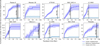 |
Fig. 2. Comparison of the cumulative number of stars in the reference neighborhood (light blue) and the cumulative number of stars that enter the cluster neighborhood (dark blue). The solid lines show the median counts over the 100 Monte Carlo traceback computations. The colored areas show the 16th and 84th percentiles of the cumulative counts. The vertical dashed lines and gray bands mark the cluster ages and uncertainties according to Bossini et al. (2019), except for the two clusters that are much older than the maximum traceback time of 100 Myr. Many more stars enter the cluster neighborhood than the reference neighborhood, suggesting that there is indeed a population of escaped cluster stars that the traceback computations are able to find. |
3.2. Cluster ages and maximum traceback time
Because there should be no fugitives older than the cluster itself, we expect to see many stars entering the cluster neighborhood in our traceback computations up to the moment of its birth, and none beyond that. The traceback times at which the cumulative count plots in Fig. 2 flatten out could then be used as estimates of the clusters’ age. We also show the cluster age estimates by Bossini et al. (2019) in Fig. 2 and it can be seen that in many cases there indeed seems to be good agreement between their cluster age estimate and the flattening of the cumulative count curve, (see, e.g., NGC 2451 A, IC 2602, or IC 2391). However, a similar flattening can be observed for Messier 39 and NGC 2516, which should be much older than our maximum traceback time of 100 Myr. This can be explained by the fact that the further back in time our traceback computations go, the larger the uncertainties of the computed phase space coordinates become. This, in turn, means the further in the past a star escaped its cluster, the less likely we are to see it enter the cluster neighborhood in our computations. Kamdar et al. (2021), who performed simulations of a Milky Way-like galaxy, find that even with perfect knowledge of the large-scale gravitational potential, stochastic encounters with giant molecular clouds still prevent accurate tracebacks of stars beyond timescales of a couple hundred million years. We should expect our useful traceback time to be even shorter. The cumulative count plots of Messier 39 and NGC 2516 indeed suggest that the timescale on which the computed phase space coordinates of the stars become too uncertain to be useful for us is tens of millions of years, which happens to be similar to the age of most of the clusters in our sample. Disentangling the resulting change in the cumulative counts’ slopes from that caused by the finite age of the clusters is not feasible, so our computations cannot be used to estimate the cluster ages, they can only be used to provide lower bounds. There are no clusters in our sample for which the number of stars having been within its neighborhood grows significantly beyond traceback times further than the cluster age estimates from Bossini et al. (2019), so our lower bounds for the cluster ages are consistent with their isochrone ages.
From the discussion above it is clear that extending the traceback computations beyond 100 Myr would not be useful. However, smaller current-day phase space coordinate uncertainties would result in smaller past coordinate uncertainties, so longer traceback times could be used with future Gaia data releases. Furthermore, it might become possible to provide traceback age estimates for some of the clusters in our sample without having to modify our traceback method itself, or at the very least the lower bounds for the cluster ages could be made more restrictive.
3.3. Hertzsprung-Russell diagrams
Figure 3 compares the members and fugitives we found with PARSEC isochrones (Bressan et al. 2012; Chen et al. 2014, 2015) on the Hertzsprung-Russell (HR) diagram. The parameters of the isochrones are listed in Table 3. The cluster members outnumber field stars in the current cluster neighborhood owing to their much larger phase space density. It is therefore not surprising that the observed HR diagrams of the members match the isochrones very well. There are a handful of clear outliers, but they all have low membership probabilities. It is more remarkable that the observed HR diagrams of the fugitives also match the same isochrones because the fugitives are spread over a large volume of phase space that contains many unrelated field stars. There are again a handful of outliers with low fugitive probabilities, but the presence of a small number of outliers is to be expected based on the estimated false positive rates listed in Table 5.
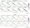 |
Fig. 3. HR diagrams of the cluster members (top ten) and fugitives (bottom ten) together with PARSEC isochrones. The isochrone ages in the panel titles are taken from Bossini et al. (2019). The metallicities of the isochrones are listed in Table 3. The fugitives agree with the isochrones just as well as the members, other than a handful of outliers with very low fugitive probabilities. The presence of such outliers is to be expected, given the estimated false positive rates listed in Table 5. |
3.4. Spatial distribution of fugitives
We now briefly compare the spatial distribution of the cluster fugitives with the structures found by Meingast et al. (2021). Figure 4 can be compared with their Fig. A.2. In most cases, the fugitives we find seem to form a stream with the inner (i.e., closer to the Galactic center) arm leading and the outer arm trailing, but this is not true for all clusters. In the cases where we do see a convincing stream, Meingast et al. (2021) also see a stream with the same orientation. The fact that the structures we find are so similar validates both our and Meingast et al. (2021) methods and also confirms that the identified structures are real.
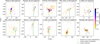 |
Fig. 4. Current-day distribution of the fugitives projected on the galactic plane. Some of the high-probability fugitives are currently far from their clusters. |
3.4.1. Platais 9
Meingast et al. (2021) found a prominent stream associated with this cluster, and the fugitives we find also tend to form a stream with the same orientation and a similar extent. The part of the stream between us and the cluster seems to be more prominent than the part behind the stream, but that is most likely due to observational biases. We also find a couple of stars with relatively high fugitive probabilities quite far from the stream. The method of Meingast et al. (2021) includes applying a clustering algorithm in position space, which prevents them from finding such stars.
3.4.2. Messier 39
The fugitives seem to form a stream with the same orientation as the stream found by Meingast et al. (2021) and a similar extent. However, the number of high-probability fugitives is rather low.
3.4.3. α Persei cluster
This is the cluster with the largest number of fugitives, but the fugitives do not seem to form a stream. It is not obvious why that would be the case. According to Bossini et al. (2019), the α Per cluster has a very similar age as Pleiades, but despite that, the distribution of the fugitives is very different. The structure Meingast et al. (2021) report is elongated, but relatively thick compared to the streams they found around many of the other clusters.
3.4.4. NGC 2451 A
The fugitives form a clear stream that has quite a large angle with respect to the trajectory of the cluster. The angle and the rough extent of the stream we see are very similar to the stream found by Meingast et al. (2021).
3.4.5. IC 2602
Once again the fugitives form a stream that is similar to the stream found by Meingast et al. (2021), but differently from the other clusters with a clear stream in this case the cluster is not centered on the stream but rather somewhat displaced laterally. This feature is also visible in the results of Meingast et al. (2021).
3.4.6. NGC 2547
Meingast et al. (2021) do not see a stream around this cluster, instead they see an extended corona. The distribution of fugitives seems to be consistent with the findings of Meingast et al. (2021), but the number of fugitives is low.
3.4.7. Blanco 1
The fugitives form a clear stream with the same orientation as the stream found by Meingast et al. (2021), but we are able to find a few fugitives farther from the cluster than anything they report. The trailing arm of the stream seems to be much longer than the leading arm, but it is not clear if this is because of the actual extent of the arms or is this appearance the result of the very small number of identified fugitives.
3.4.8. IC 2391
The fugitives seem to form a stream with an orientation roughly similar to that found by Meingast et al. (2021). However, the spatial extent of the fugitives is somewhat smaller than the structure they found.
3.4.9. NGC 2516
The fugitives form a clear stream with an orientation very similar to the stream found by Meingast et al. (2021). The spatial extent of the bulk of the fugitives is somewhat smaller, but there are a handful of stars with moderate fugitive probabilities closer to us and farther from the cluster than the end of the stream Meingast et al. (2021) find.
3.4.10. Pleiades
The fugitives seem to form a clear stream, but differently from the other clusters it is the inner arm of the stream that is trailing and the outer arm that is leading. This orientation matches the orientation Meingast et al. (2021) find, but their results do not include the inner trailing arm, whereas we find many fugitives there.
4. Discussion
4.1. Radial velocity as the dominant source of uncertainty
Figure 5 shows the cluster member coordinates in the XY- and UV-planes. It can be seen that all clusters are strongly elongated along the line of sight in velocity space. This means that many stars have nominal radial velocities that place them outside the cluster neighborhood, but the radial velocity uncertainty is large enough that they are placed inside the neighborhood in a large fraction of the Monte Carlo samples described in Sect. 2.1. The fact that the clusters are elongated only along the line of sight but not tangentially to it means that the tangential velocity uncertainty is much smaller. Furthermore, no clear elongation is visible in position space. This means that the radial velocity is the dominant source of uncertainty and applying quality cuts based on commonly used criteria such as RUWE would not improve our results.
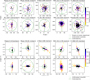 |
Fig. 5. Current-day position (top ten) and velocity (bottom ten) distribution of the members projected on the galactic plane. The green arrows show what a cluster’s velocity components would be if its radial velocity were larger by 3 km s−1 and therefore indicate the line-of-sight directions for each cluster. From the fact that the clusters appear to be strongly elongated along the line of sight in velocity space while not being visibly elongated in position space, it is apparent that the radial velocity uncertainty is much larger than the uncertainties of other phase space coordinates. Blanco 1 is at a very high galactic latitude, so the apparent cluster elongation in velocity space is mostly along the W axis and is not prominent in the U − V plot. |
4.2. Probability threshold value, pmin
Our definitions of fugitives and members are meant to both exclude unrelated field stars and also to distinguish stars currently very close to a cluster in phase space, which can be associated with the cluster without traceback computations, from the more distant stars whose connection to the cluster is not obvious. We used a single parameter for dividing the stars into these three groups with a somewhat arbitrary value of pmin = 0.1, and using a different value might reclassify some of our members as fugitives or some of our fugitives as members. That being said, there are two groups that are simple to interpret regardless of the adopted value of pmin. First, stars with pm = 0 cannot be considered to be members. Second, stars with pf = pm cannot be classified as fugitives because either pm > pmin and they qualify as members, or pmin ≥ pf and they qualify as unrelated stars. Stars with pf > pm > 0 could be classified as members or fugitives depending on the adopted probability threshold value pmin.
We can see in Fig. 6, however, that the majority of stars are either on or very close to the vertical line pm = 0, meaning they cannot be cluster members, or on or very close to the main diagonal pf = pm, meaning they cannot be considered fugitives. The number of stars that do not clearly belong to either of the two groups is very low, with the exception of NGC 2516, which means that whether stars get classified as members or fugitives of the other nine clusters is not sensitive to the exact value of pmin. NGC 2516 is the most distant of the ten clusters we considered, so the stars associated with it have the largest uncertainties in their phase space coordinates, but even in that cluster the number of stars that could be classified as members or fugitives is not too large, and most of those have low membership and fugitive probabilities regardless.
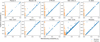 |
Fig. 6. Comparison of fugitive and membership probabilities of members and fugitives. Stars close to the vertical line pm = 0 are clearly not members, and those close to the main diagonal are not fugitives. Stars in between could be classified as members or fugitives depending on the value of pmin, but the number of such stars is very low. The only cluster where there are more than a handful of in-between stars is NGC 2516. This is due to the fact that it is the farthest away and, therefore, its stars have the most uncertain phase space coordinates. Even so, most of the ambiguous stars have low membership and fugitive probabilities. |
4.3. Size of the cluster neighborhood
The extent of a star cluster in phase space is nonzero, and measurement uncertainties make the cluster appear even more spread out. Performing our analysis using a neighborhood that is too small would therefore cause us to miss cluster members and fugitives. A very large neighborhood, however, leads to a very large field star contamination rate. Our choice must reflect these two competing incentives, meaning it should be large enough to find as many true fugitives as possible while keeping the false positive rate at an acceptable level.
From Table 5 we can see that with the neighborhood radii we used, 15 pc and 3 km s−1, the median false positive rate of the ten clusters is 6% and the maximum is 14%. We consider these values to be acceptable and see no reason to use smaller neighborhoods. If we set the neighborhood radii to 20 pc and 3 km s−1, then the median false positive rate of the clusters is 11% and the maximum 33%. If the neighborhood radii are 15 pc and 4 km s−1, then the median false positive rate is 15.5% and maximum 29%. We consider the false positive rates to be too large to justify using the larger neighborhood radii.
4.4. Parameters of the orbit of the Sun
Converting the heliocentric coordinates observed by Gaia to galactocentric coordinates used in the traceback computations requires knowing the parameters of the orbit of the Sun. Changing these parameters also changes the orbits of all other stars. There are a few reasons to believe that our results should not be very sensitive to such changes:
-
If a star and a cluster are on similar orbits with one set of solar orbit parameters, then they are also on similar orbits with some slightly different set of parameters.
-
The time when a star enters the cluster neighborhood might change, but we are only interested in whether the star enters the neighborhood before some maximum traceback time or not.
-
How close a star approaches a cluster might change, but we are only interested in whether the star enters the cluster neighborhood or not.
It is, however, important to verify that these assumptions indeed hold for our data. We therefore performed an additional traceback computation by assuming different parameter values for the orbit of the Sun, listed in Table 6, with correspondingly different galactocentric cylindrical phase space coordinates of the stars and clusters. We did not modify the Galactic potential we used, but the change in the galactocentric coordinates resulted in a change of the gravitational potential at the clusters’ locations. We note that this is probably a worst-case scenario, as this choice means that the Sun’s velocity with respect to the local standard of rest changed by ∼13 km s−1, with a similar effect for all the stars and clusters we considered. Figure 7 compares the fugitive probabilities obtained from the two tracebacks. The results are overall very similar, as demonstrated by the Pearson correlation coefficient values (in the panel titles) being close to one. We conclude that our results are indeed not sensitive to the values of the parameters of the orbit of the Sun.
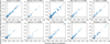 |
Fig. 7. Comparison of fugitive probabilities computed with the nominal parameters of the orbit of the Sun, as listed in Table 1, and with the alternative parameters listed in Table 6. Only stars with a fugitive probability pf > 0.1 in either traceback and with a membership probability pm ≤ 0.1 are included. The Pearson correlation coefficients (in the panel titles) are close to 1, meaning the fugitive probabilities are not sensitive to the exact values of the solar orbit parameters. |
Alternative parameters of the solar orbit, also used by Meingast et al. (2021).
4.5. Completeness and limitations
In the Gaia era it is the availability of radial velocities that limits the completeness of the stellar sample that can be included in the traceback computations. Although it is possible to augment Gaia radial velocities with other catalogs, it would still remain true that the completeness would be lower for fainter sources. Furthermore, because completeness is a function of apparent magnitude, it is more difficult to find fugitives that are behind their cluster (farther from us) compared to the fugitives in front of it (closer to us).
Methods that do not require radial velocity measurements, such as the convergent point method, suffer less from these drawbacks and therefore allow greater completeness. But some stars that the convergent point method would associate with a cluster might be easily recognizable as unrelated field stars if radial velocity measurements were available. On the other hand, methods incorporating chemical tagging in addition to kinematic data have the potential of producing fugitive samples with much lower field star contamination rates than the traceback method, but they require spectra with even higher quality than what is needed for radial velocity, measurements. The convergent point method, the traceback method and methods combining kinematic data with chemical tagging therefore form a sequence with increasing reliability at the cost of decreasing completeness.
It might also be advantageous to combine the methods. Some version of the convergent point method could be used to relatively easily exclude stars that are clearly kinematically distinct from the cluster. Our traceback method could then be used to further refine the sample and to quantify individual fugitive probabilities and the field star contamination rate. High-probability fugitives could in turn be good candidates for spectroscopic followup that is required for strong chemical tagging.
5. Summary
We present a new method of identifying stars that have escaped from nearby open clusters in the last few ten million years, which we have applied to ten nearby young clusters. Our method is based on the assumptions that the fugitives have been close to the cluster in phase space in the past, but we do not assume the fugitives are close to the cluster at present. We show how the fugitive probability of each individual star can be estimated with a straightforward Monte Carlo procedure. We also show how the field star contamination rate can be estimated for each cluster by counting stars around a reference point, and describe how a suitable reference point can be chosen.
Our method requires a model of the gravitational potential of the Galaxy and the parameters of the orbit of the Sun. They are constrained by observations, and we demonstrate that having exact values is not critical. Our method also requires choosing the size of the cluster neighborhood in phase space. Rough values are suggested by observations of open clusters, and the final choice can be evaluated using the field star contamination rate. We additionally adopted a probability threshold to avoid cluttering our analysis with stars with very low fugitive probabilities, and although we also used the same threshold value to distinguish cluster members from fugitives, we show that this division does not strongly depend on the exact value of the threshold.
Our method is able to provide lower bounds of cluster ages. The bounds we obtain with Gaia DR3 data are not very restrictive, but all are consistent with the isochrone ages from Bossini et al. (2019). Furthermore, the fugitives we identify are consistent with the cluster isochrones on the HR diagram. The spatial distribution of the fugitives we identify seems to be consistent with the structures found by Meingast et al. (2021). In cases where the extended stellar structures they found had a convincing preferred orientation, we also tend to see an elongated structure with a very similar orientation.
A shortcoming of our method is that it is reliant on Gaia radial velocity measurements. The relatively small number of stars with such measurements limits the completeness of our fugitive sample. Additionally, for stars that do have such measurements available, the radial velocity uncertainty tends to be the main contributor of their phase space coordinate uncertainty, which limits the useful maximum traceback time. Despite that, our method is already capable of complementing the fugitive lists obtained with other methods and can be applied to many clusters relatively easily. Future Gaia data releases are expected to include more stars with radial velocity measurements and to have smaller uncertainties for the stars with measurements available already. Our method will be able to take advantage of such richer data sets with only trivial modifications.
Acknowledgments
We thank the anonymous referee for helpful comments. P.M. gratefully acknowledges support from project grants from the Swedish Research Council (Vetenskaprådet, Reg: 2017-03721; 2021-04153). Some of the computations in this project were completed on computing equipment bought with a grant from The Royal Physiographic Society in Lund. This research has made use of NASA’s Astrophysics Data System. This work made use of astropy: a community-developed core Python package and an ecosystem of tools and resources for astronomy (Astropy Collaboration 2013, 2018, 2022). This work made use of matplotlib (Hunter 2007) and numpy (Harris et al. 2020).
References
- Aigrain, S., Hodgkin, S., Irwin, J., et al. 2007, MNRAS, 375, 29 [NASA ADS] [CrossRef] [Google Scholar]
- Astropy Collaboration (Robitaille, T. P., et al.) 2013, A&A, 558, A33 [NASA ADS] [CrossRef] [EDP Sciences] [Google Scholar]
- Astropy Collaboration (Price-Whelan, A. M., et al.) 2018, AJ, 156, 123 [Google Scholar]
- Astropy Collaboration (Price-Whelan, A. M., et al.) 2022, ApJ, 935, 167 [NASA ADS] [CrossRef] [Google Scholar]
- Beccari, G., Boffin, H. M. J., Jerabkova, T., et al. 2018, MNRAS, 481, L11 [Google Scholar]
- Bennett, M., & Bovy, J. 2019, MNRAS, 482, 1417 [NASA ADS] [CrossRef] [Google Scholar]
- Binney, J., Gerhard, O., & Spergel, D. 1997, MNRAS, 288, 365 [NASA ADS] [CrossRef] [Google Scholar]
- Bossini, D., Vallenari, A., Bragaglia, A., et al. 2019, A&A, 623, A108 [NASA ADS] [CrossRef] [EDP Sciences] [Google Scholar]
- Bouma, L. G., Curtis, J. L., Hartman, J. D., Winn, J. N., & Bakos, G. Á. 2021, AJ, 162, 197 [NASA ADS] [CrossRef] [Google Scholar]
- Bovy, J. 2015, ApJS, 216, 29 [NASA ADS] [CrossRef] [Google Scholar]
- Bressan, A., Marigo, P., Girardi, L., et al. 2012, MNRAS, 427, 127 [NASA ADS] [CrossRef] [Google Scholar]
- Cantat-Gaudin, T., & Anders, F. 2020, A&A, 633, A99 [NASA ADS] [CrossRef] [EDP Sciences] [Google Scholar]
- Carrera, R., Bragaglia, A., Cantat-Gaudin, T., et al. 2019, A&A, 623, A80 [NASA ADS] [CrossRef] [EDP Sciences] [Google Scholar]
- Chen, Y., Girardi, L., Bressan, A., et al. 2014, MNRAS, 444, 2525 [Google Scholar]
- Chen, Y., Bressan, A., Girardi, L., et al. 2015, MNRAS, 452, 1068 [Google Scholar]
- Conrad, C., Scholz, R. D., Kharchenko, N. V., et al. 2017, A&A, 600, A106 [NASA ADS] [CrossRef] [EDP Sciences] [Google Scholar]
- Crundall, T. D., Ireland, M. J., Krumholz, M. R., et al. 2019, MNRAS, 489, 3625 [Google Scholar]
- Dinnbier, F., Kroupa, P., Šubr, L., & Jeřábková, T. 2022, ApJ, 925, 214 [NASA ADS] [CrossRef] [Google Scholar]
- Drimmel, R., & Poggio, E. 2018, Res. Notes Am. Astron. Soc., 2, 210 [Google Scholar]
- Farias, J. P., Tan, J. C., & Eyer, L. 2020, ApJ, 900, 14 [NASA ADS] [CrossRef] [Google Scholar]
- Gaia Collaboration (Babusiaux, C., et al.) 2018, A&A, 616, A10 [NASA ADS] [CrossRef] [EDP Sciences] [Google Scholar]
- Gaia Collaboration (Brown, A. G. A., et al.) 2021, A&A, 649, A1 [NASA ADS] [CrossRef] [EDP Sciences] [Google Scholar]
- Ginsburg, A., Sipőcz, B. M., Brasseur, C. E., et al. 2019, AJ, 157, 98 [Google Scholar]
- GRAVITY Collaboration (Abuter, R., et al.) 2018, A&A, 615, L15 [NASA ADS] [CrossRef] [EDP Sciences] [Google Scholar]
- Harris, C. R., Millman, K. J., van der Walt, S. J., et al. 2020, Nature, 585, 357 [NASA ADS] [CrossRef] [Google Scholar]
- Hunter, J. D. 2007, Comput. Sci. Eng., 9, 90 [NASA ADS] [CrossRef] [Google Scholar]
- Jerabkova, T., Boffin, H. M. J., Beccari, G., et al. 2021, A&A, 647, A137 [NASA ADS] [CrossRef] [EDP Sciences] [Google Scholar]
- Kamdar, H., Conroy, C., & Ting, Y. S. 2021, ApJ, submitted [arXiv:2106.02050] [Google Scholar]
- Kroupa, P., Jerabkova, T., Thies, I., et al. 2022, MNRAS, 517, 3613 [CrossRef] [Google Scholar]
- Krumholz, M. R., McKee, C. F., & Bland -Hawthorn, J., 2019, ARA&A, 57, 227 [Google Scholar]
- Lada, C. J., & Lada, E. A. 2003, ARA&A, 41, 57 [Google Scholar]
- Lindegren, L., Bastian, U., Biermann, M., et al. 2021, A&A, 649, A4 [EDP Sciences] [Google Scholar]
- Magrini, L., Randich, S., Kordopatis, G., et al. 2017, A&A, 603, A2 [NASA ADS] [CrossRef] [EDP Sciences] [Google Scholar]
- Meingast, S., Alves, J., & Rottensteiner, A. 2021, A&A, 645, A84 [NASA ADS] [CrossRef] [EDP Sciences] [Google Scholar]
- Netopil, M., Paunzen, E., Heiter, U., & Soubiran, C. 2016, A&A, 585, A150 [NASA ADS] [CrossRef] [EDP Sciences] [Google Scholar]
- Piskunov, A. E., Kharchenko, N. V., Röser, S., Schilbach, E., & Scholz, R. D. 2006, A&A, 445, 545 [CrossRef] [EDP Sciences] [Google Scholar]
- Price-Whelan, A. M. 2017, J. Open Source Software, 2, 388 [NASA ADS] [CrossRef] [Google Scholar]
- Röser, S., & Schilbach, E. 2019, A&A, 627, A4 [NASA ADS] [CrossRef] [EDP Sciences] [Google Scholar]
- Röser, S., & Schilbach, E. 2020, A&A, 638, A9 [NASA ADS] [CrossRef] [EDP Sciences] [Google Scholar]
- Röser, S., Schilbach, E., & Goldman, B. 2019, A&A, 621, L2 [NASA ADS] [CrossRef] [EDP Sciences] [Google Scholar]
- Schoettler, C., de Bruijne, J., Vaher, E., & Parker, R. J. 2020, MNRAS, 495, 3104 [NASA ADS] [CrossRef] [Google Scholar]
- Schönrich, R., Binney, J., & Dehnen, W. 2010, MNRAS, 403, 1829 [NASA ADS] [CrossRef] [Google Scholar]
- Soubiran, C., Cantat-Gaudin, T., Romero-Gómez, M., et al. 2018, A&A, 619, A155 [NASA ADS] [CrossRef] [EDP Sciences] [Google Scholar]
- Spina, L., Randich, S., Magrini, L., et al. 2017, A&A, 601, A70 [NASA ADS] [CrossRef] [EDP Sciences] [Google Scholar]
- Wenger, M., Ochsenbein, F., Egret, D., et al. 2000, A&AS, 143, 9 [NASA ADS] [CrossRef] [EDP Sciences] [Google Scholar]
Appendix A: Rough cluster coordinates
Rough values of the cluster coordinates queried from SIMBAD (Wenger et al. 2000) using astroquery (Ginsburg et al. 2019) are listed in Table A.1. These values were used as initial guesses for the procedure described in Sect. 2.3 to obtain the nominal cluster coordinates, so their exact values are not critical.
Rough values of the cluster coordinates.
Appendix B: Distribution of the fugitives on the sky
Figure B.1 shows the distribution of the cluster fugitives on the sky and demonstrates their large extent.
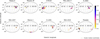 |
Fig. B.1. Current-day distribution of the fugitives on the sky. |
All Tables
Limits for the coordinates of the stars included in the initial traceback computation.
False positive rates, which are the medians of the false positive rates of the Monte Carlo tracebacks, shown with the 16th and 84th percentiles.
All Figures
|
Fig. 1. Galactocentric cylindrical coordinates and the heliocentric Cartesian coordinates. The z (galactocentric) and Z (heliocentric) coordinates are almost perpendicular to the plane of the figure. The Sun is located at (R, ϕ, z) = (8000 pc, 180° ,14 pc), and the Galactic center is located at (X, Y, Z) = (8000 pc, 0 pc, 0 pc). |
| In the text | |
|
Fig. 2. Comparison of the cumulative number of stars in the reference neighborhood (light blue) and the cumulative number of stars that enter the cluster neighborhood (dark blue). The solid lines show the median counts over the 100 Monte Carlo traceback computations. The colored areas show the 16th and 84th percentiles of the cumulative counts. The vertical dashed lines and gray bands mark the cluster ages and uncertainties according to Bossini et al. (2019), except for the two clusters that are much older than the maximum traceback time of 100 Myr. Many more stars enter the cluster neighborhood than the reference neighborhood, suggesting that there is indeed a population of escaped cluster stars that the traceback computations are able to find. |
| In the text | |
|
Fig. 3. HR diagrams of the cluster members (top ten) and fugitives (bottom ten) together with PARSEC isochrones. The isochrone ages in the panel titles are taken from Bossini et al. (2019). The metallicities of the isochrones are listed in Table 3. The fugitives agree with the isochrones just as well as the members, other than a handful of outliers with very low fugitive probabilities. The presence of such outliers is to be expected, given the estimated false positive rates listed in Table 5. |
| In the text | |
|
Fig. 4. Current-day distribution of the fugitives projected on the galactic plane. Some of the high-probability fugitives are currently far from their clusters. |
| In the text | |
|
Fig. 5. Current-day position (top ten) and velocity (bottom ten) distribution of the members projected on the galactic plane. The green arrows show what a cluster’s velocity components would be if its radial velocity were larger by 3 km s−1 and therefore indicate the line-of-sight directions for each cluster. From the fact that the clusters appear to be strongly elongated along the line of sight in velocity space while not being visibly elongated in position space, it is apparent that the radial velocity uncertainty is much larger than the uncertainties of other phase space coordinates. Blanco 1 is at a very high galactic latitude, so the apparent cluster elongation in velocity space is mostly along the W axis and is not prominent in the U − V plot. |
| In the text | |
|
Fig. 6. Comparison of fugitive and membership probabilities of members and fugitives. Stars close to the vertical line pm = 0 are clearly not members, and those close to the main diagonal are not fugitives. Stars in between could be classified as members or fugitives depending on the value of pmin, but the number of such stars is very low. The only cluster where there are more than a handful of in-between stars is NGC 2516. This is due to the fact that it is the farthest away and, therefore, its stars have the most uncertain phase space coordinates. Even so, most of the ambiguous stars have low membership and fugitive probabilities. |
| In the text | |
|
Fig. 7. Comparison of fugitive probabilities computed with the nominal parameters of the orbit of the Sun, as listed in Table 1, and with the alternative parameters listed in Table 6. Only stars with a fugitive probability pf > 0.1 in either traceback and with a membership probability pm ≤ 0.1 are included. The Pearson correlation coefficients (in the panel titles) are close to 1, meaning the fugitive probabilities are not sensitive to the exact values of the solar orbit parameters. |
| In the text | |
|
Fig. B.1. Current-day distribution of the fugitives on the sky. |
| In the text | |
Current usage metrics show cumulative count of Article Views (full-text article views including HTML views, PDF and ePub downloads, according to the available data) and Abstracts Views on Vision4Press platform.
Data correspond to usage on the plateform after 2015. The current usage metrics is available 48-96 hours after online publication and is updated daily on week days.
Initial download of the metrics may take a while.