| Issue |
A&A
Volume 679, November 2023
|
|
|---|---|---|
| Article Number | A65 | |
| Number of page(s) | 23 | |
| Section | Stellar atmospheres | |
| DOI | https://doi.org/10.1051/0004-6361/202346783 | |
| Published online | 10 November 2023 | |
Effects of magnetic fields on the center-to-limb variation in solar-type stars
1
Landessternwarte – Zentrum für Astronomie der Universität Heidelberg,
Königstuhl 12,
69117
Heidelberg,
Germany
e-mail: This email address is being protected from spambots. You need JavaScript enabled to view it.
2
Leibniz-Institut für Astrophysik Potsdam,
An der Sternwarte 16,
14482
Potsdam,
Germany
3
Theoretical Astrophysics, Department of Physics and Astronomy, Uppsala University,
Box 516,
751 20
Uppsala,
Sweden
Received:
1
May
2023
Accepted:
3
August
2023
Abstract
Context. High-precision photometry of exoplanet transits obtained with the Kepler satellite allows one to derive information on the center-to-limb variation (CLV) of the host stars. Recent analyses indicate a small but systematic discrepancy between observations and theoretical expectations based on detailed multidimensional model atmospheres. It has been hypothesized that the discrepancy is related to the neglect of magnetic fields in the models.
Aims. Our goal is to test the above hypothesis for solar-like stars. We further intend to quantify the consequences for interferometry, and the possibility of extracting information at the level of stellar magnetic activity from the CLV.
Methods. We constructed a sequence of multidimensional models including magnetic fields of varying strengths. We derived theoretical predictions on the CLV, taking into account factors like the observational passband, stellar sphericity, the methodology of the light curve analysis, and interstellar extinction.
Results. The models predict a relative brightening of the stellar limb with increasing magnetic field strength, which qualitatively goes in the direction of reducing the mismatch between observation and theory. Quantitatively, however, the mismatch is not fully eliminated. Interstellar extinction on a level AV ≲ 1 mag has little impact on the CLV and is largely degenerate with the influence of magnetic fields. Global magnetic activity at field strengths ≲300 G influences interferometric radius measurements to ≲1%. We emphasize that our results refer to measurements taken in the Kepler passband.
Conclusions. The presence of magnetic activity appears to be a plausible explanation for the present discrepancy between observation and theory. The still-present partial mismatch needs to be understood. To this end, we point to improvements in modeling and wishes for more observational data of active stars, including spectral information.
Key words: magnetohydrodynamics (MHD) / stars: atmospheres / stars: solar-type / techniques: photometric
© The Authors 2023
 Open Access article, published by EDP Sciences, under the terms of the Creative Commons Attribution License (https://creativecommons.org/licenses/by/4.0), which permits unrestricted use, distribution, and reproduction in any medium, provided the original work is properly cited.
This article is published in open access under the Subscribe to Open model. This email address is being protected from spambots. You need JavaScript enabled to view it. to support open access publication.
1 Introduction
The analysis of the light curves of planetary transits makes it possible for information to be derived on the center-to-limb variation (hereafter CLV) of stars. Photometry from space has given particular impetus to this observational technique (e.g., Sing et al. 2008; Howarth 2011; Csizmadia et al. 2013; Espinoza & Jordán 2016; Patel & Espinoza 2022). In two investigations (Maxted 2018, 2023, hereafter M18 and M23, respectively), P. Maxted analyzed high-quality light curves of transiting systems observed during the K1 phase of the Kepler satellite mission (Borucki et al. 2010). He selected non-binary FGKM-type host stars harboring hot Jupiters with atmospheric parameters derived from high-resolution spectroscopy. The short orbital periods typically allowed for the observation of hundreds of transits that were co-added to improve the photometric signal-to-noise ratio.
Besides the orbital characteristics and planetary radius, his analysis provided information on the limb darkening (LD) of the host star in the form of limb darkening coefficients (LDCs) of an assumed LD law. He compared the observational LDCs to predicted LDCs based on three-dimensional (3D), hydro-dynamical model atmospheres calculated with the STAGGER code (Magic et al. 2013; Chiavassa et al. 2018). The correspondence was good, except for small systematic offsets that Maxted hypothesized to be related to the neglect of magnetic fields in the STAGGER models. It is this hypothesis that we intend to check the plausibility of in this investigation.
Magneto-hydrodynamical (MHD) model atmospheres are nowadays routinely constructed for cool main-sequence stars, ranging from models representing patches on the stellar surface exhibiting various levels of magnetic activity (e.g., Carlsson et al. 2004; Stein & Nordlund 2006; Schüssler & Vögler 2006; Vögler & Schüssler 2007; Steiner et al. 2014; Beeck et al. 2015; Norris et al. 2017; Salhab et al. 2018; Bhatia et al. 2022) to models of complete sun- or starspots (e.g., Rempel et al. 2009; Chen et al. 2017; Panja et al. 2020, 2021).
To test Maxted’s hypothesis, we constructed a sequence of MHD models calculated with the CO5BOLD code (Freytag et al. 2012), and based on these models subsequently performed spectral synthesis computations reproducing the Kepler photometry. Our models fall into the category of models representing surface patches of given magnetic activity. We emphasize that our investigation is a pilot study, and the applied MHD models are restricted to solar conditions in terms of surface gravity, metallicity, and entropy encountered in the deep convective envelope; nevertheless, they cover a large range of activity levels. The quality of the models is limited in terms of spatial resolution as well as the configuration of the magnetic field, and the synthetic photometry is not fully comprehensive. As a consequence, we had to devise procedures to mitigate shortcomings. The description of these takes up some room; however, we think that some of the presented ideas are interesting in their own right. Some precursory work based on a subset of the MHD runs used here was already presented in a Master’s thesis by Ji (2021). Moreover, in an ongoing parallel investigation at the Max-Planck Institute for Solar System Research, results have been obtained that are largely consistent with what is presented in this paper (Kostogryz, Shapiro, Witzke et al. 2023, priv. comm.).
A few words about the nomenclature we use in this article. We refer to hydrodynamical model atmospheres that do not include magnetic fields as “HD” models, and models that include magnetic fields as “MHD” models. When referring to radiation quantities like specific intensities and fluxes (first angular moment of the intensity), we always refer to values integrated over the Kepler passband if not stated otherwise.
This paper is organized as follows: we start with a long section on the methodological aspects, which describes the applied LD laws, HD and MHD models, spectral synthesis calculations, how we deal with the effects of stellar sphericity, and the normalization of observational data, as well as light curve construction and fitting. We tried to keep the methodology section compact by moving details in our argumentations to appendices. The following section on the obtained results primarily illustrates the partial match between theory and observations. We also discuss the effects of interstellar extinction and the impact of magnetic activity on interferometric measurements of stellar diameters. In the final section, we present the obtained conclusions together with ideas for further work on the subject. Among the appendices, the last one lists the synthetic intensities underlying the investigated LD laws.
2 Methodological aspects
Arriving at the final comparison between observational and theoretical data involves a number of intricate steps. To keep an overview, we summarize the chain of events briefly in Fig. 1.
2.1 Limb-darkening laws
In this work, we make use of the LD laws introduced by Claret (2000) and Hestroffer (1997). These LD laws describe the functional dependence of the emergent intensity, I, toward the observer as a function of the position on the apparent stellar disk given by µ, the cosine of the angle between the line-of-sight and radial (equivalently vertical) direction. Claret originally proposed a fourth order polynomial in  . In some cases we will go from N = 4 to the higher polynomial order N = 6, as given by
![Mathematical equation: $ I\left( \mu \right) = I\left( 1 \right)\,\left[ {1 - \sum\limits_{j = 1}^N {{c_j}} \left( {1 - {{\sqrt \mu }^j}} \right)} \right]. $](/articles/aa/full_html/2023/11/aa46783-23/aa46783-23-eq2.png) (1)
(1)
The cj are free LDCs controlling the shape of the LD law. We will use the names Claret-4 or Claret-6 for these laws. As is apparent from Eq. (1), we opted to work with absolute intensities (not intensity ratios) so that the intensity, I(1) (the argument of the intensity here and in the following four equations is µ), at the disk center appears as an additional parameter in the relation. This was motivated by the desire to treat all the intensities computed at various disk positions on an equal footing, and not assign a special status to the intensity at the disk center.
Besides the disk center intensity, the LD law of Hestroffer contains only two free coefficients, viz. (c, α):
![Mathematical equation: $ I\left( \mu \right) = I\left( 1 \right)\,\left[ {1 - c\,\left( {1 - {\mu ^\alpha }} \right)} \right]. $](/articles/aa/full_html/2023/11/aa46783-23/aa46783-23-eq3.png) (2)
(2)
Hestroffer argued in the context of interferometric observations that this so-called power-2 law can provide a good representation of the LD despite its small number of free parameters. When analyzing planetary transits, M18 finds that the derived c and α parameters are often closely correlated, and proposes an alternative parameterization of the power-2 law defining the two parameters
![Mathematical equation: $ \matrix{ {{h_1} \equiv {{I\left( {{1 \mathord{\left/ {\vphantom {1 2}} \right. \kern-\nulldelimiterspace} 2}} \right)} \mathord{\left/ {\vphantom {{I\left( {{1 \mathord{\left/ {\vphantom {1 2}} \right. \kern-\nulldelimiterspace} 2}} \right)} {I\left( 1 \right)\,\,}}} \right. \kern-\nulldelimiterspace} {I\left( 1 \right)\,\,}}} & {{\rm{and}}} & {{h_2} \equiv {{\left[ {I\left( {{1 \mathord{\left/ {\vphantom {1 2}} \right. \kern-\nulldelimiterspace} 2}} \right) - I\left( 0 \right)} \right]} \mathord{\left/ {\vphantom {{\left[ {I\left( {{1 \mathord{\left/ {\vphantom {1 2}} \right. \kern-\nulldelimiterspace} 2}} \right) - I\left( 0 \right)} \right]} {I\left( 1 \right)}}} \right. \kern-\nulldelimiterspace} {I\left( 1 \right)}}} \cr } $](/articles/aa/full_html/2023/11/aa46783-23/aa46783-23-eq4.png) (3)
(3)
that are less correlated and lead to more stable fits. M18 provides explicit formulae for the transformation between the parameter pairs (c, α) and (h1, h2). Later it is realized that the definition of h2 poses a problem, since its calculation requires information on the intensity at the extreme stellar limb at µ = 0 that is observationally as well as theoretically difficult to access. For that reason an alternative parameter, h2pp is introduced that does not require information on the extreme limb
![Mathematical equation: $ {h_{2{\rm{pp}}}} \equiv \,\left[ {I\left( {{1 \mathord{\left/ {\vphantom {1 2}} \right. \kern-\nulldelimiterspace} 2}} \right) - I\left( {{1 \mathord{\left/ {\vphantom {1 {10}}} \right. \kern-\nulldelimiterspace} {10}}} \right)} \right]\,I\left( 1 \right). $](/articles/aa/full_html/2023/11/aa46783-23/aa46783-23-eq5.png) (4)
(4)
M23 finds that limb-darkening curves derived from planetary transits are fairly imprecise for µ ≲ 0.2, which leads him to introduce parameters (h′1, h′2), taking recourse to intensity values at µ ≳ 0.2 only
![Mathematical equation: $ \matrix{ {{{h'}_1} \equiv {{I\left( {{2 \mathord{\left/ {\vphantom {2 3}} \right. \kern-\nulldelimiterspace} 3}} \right)} \mathord{\left/ {\vphantom {{I\left( {{2 \mathord{\left/ {\vphantom {2 3}} \right. \kern-\nulldelimiterspace} 3}} \right)} {I\left( 1 \right)}}} \right. \kern-\nulldelimiterspace} {I\left( 1 \right)}}} & {{\rm{and}}} & {{{h'}_2} \equiv {{\left[ {I\left( {{2 \mathord{\left/ {\vphantom {2 3}} \right. \kern-\nulldelimiterspace} 3}} \right) - I\left( {{1 \mathord{\left/ {\vphantom {1 3}} \right. \kern-\nulldelimiterspace} 3}} \right)} \right]} \mathord{\left/ {\vphantom {{\left[ {I\left( {{2 \mathord{\left/ {\vphantom {2 3}} \right. \kern-\nulldelimiterspace} 3}} \right) - I\left( {{1 \mathord{\left/ {\vphantom {1 3}} \right. \kern-\nulldelimiterspace} 3}} \right)} \right]} {I\left( 1 \right)}}} \right. \kern-\nulldelimiterspace} {I\left( 1 \right)}}.} \cr } $](/articles/aa/full_html/2023/11/aa46783-23/aa46783-23-eq6.png) (5)
(5)
The definition of the parameters h2 and h2pp motivated us to model the shape of the LD curve at the stellar limb as closely as possible. We developed approximate ways to calculate the intensity profile at the stellar limb, and correct for the effects of sphericity not included in the 3D models, as detailed in later sections. A final important point, which is related to the fact that the shape of the power-2 LD law is fully determined by two parameters: any pair of (independent) parameters can be chosen to describe its shape, and it is possible to transform between pairs. We used this feature to occasionally switch from (Al , A2) to (h′1, h′2), which we mostly use in later plots.
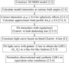 |
Fig. 1 Processing steps of the CLV analysis. References to the most relevant sections of the steps are given in angular brackets. |
Summary of the properties of the magnetic models.
2.2 CO5BOLD MHD and HD simulations
We computed 3D Cartesian “local-box” model atmospheres with the radiation-magneto-hydrodynamics code CO5BOLD (for further information on the code and applications see Freytag et al. 2012). We constructed a series of nine MHD models representing the solar atmosphere from field-free to sun-spot (umbral) conditions (see Table 1 for their field strengths). The chemical composition of all MHD models is solar, as is their surface gravity. The vertical magnetic flux through the atmosphere was set by the initial conditions of a simulation run and was preserved during the evolution of the flow. Besides a fixed magnetic flux, the field geometry was constrained by the condition that field lines had to pass vertically through the top and bottom boundaries. In this pilot study a rather low number of 140 × 140 × 150 spatial grid points was used in the x × y × z-direction. In Appendix В we further comment on the impact of resolution and field configuration. The computational domain had an extent of 5.6 × 5.6 × 2.25 Mm3, covering the optically thin photosphere and the uppermost part of the convective envelope. Periodic side boundaries were applied, and the top and bottom boundaries were made open to the plasma flow. The wavelength dependence of the radiative transfer was described by applying a multigroup technique (Nordlund 1982; Ludwig et al. 1994; Trampedach et al. 2013; Kostogryz et al. 2022) using 12 opacity bins. When a run had reached a statistically steady state, its evolution was recorded over the durations given in Table 1, which correspond to many convective turnover times. In this paper we refer to a specific MHD model by “BXXXX” in which “XXXX” stands for the field strength applied in the model.
The setup of the MHD models described above reflects the standard way in which local-box MHD models are typically constructed nowadays. Table 1 lists the resulting effective temperatures, Teff of the MHD models, showing first a modest increase of Teff with increasing field strength and then a strong drop, as expected toward sunspot like conditions (see also Vögler 2005). The substantial change of Teff with field strength brings up the question of what the term “solar conditions” means in the present context. The models have an open lower boundary, allowing the in- and outflow of plasma. The entropy of inflowing material being convectively transported toward the surface is decisive for the resulting Teff of a model. Here we applied a fixed entropy of 1.7734 × 10⁹erg g−1 K−1 in all models. With this value and in field-free conditions, a model results with close to solar Teff. Together with the fixed solar surface gravity and solar atmospheric chemical composition, this is what we mean by “solar conditions”, demoting Teff from a fundamental control parameter to an outcome of a simulation run. We will later see that this choice has an important practical consequence.
Figure 2 shows horizontally (on surfaces of equal Rosseland optical depth) and temporally averaged temperature profiles for the nine MHD models. At magnetic fields strength В ≲ 400 G one recognizes a heating of the upper photosphere, also reflected in an increase in the effective temperature of a model. The increasingly strong suppression of the convective motions taking place at higher field strengths leads to a cooling of the structure. In all cases the T(τ)-relation is monotonous so that one may also expect a monotonous run of the emergent intensity with μ; it turns out that this is indeed not the case at high field strengths. Figure 3 depicts the spatial-temporal temperature fluctuation present in the nine MHD models. There is an overall increase in the level of fluctuations with increasing field strength, except for the models with strongest field. We see later that this reflects the level of temporal fluctuations of the emergent intensity.
Figure 4 shows images of the bolometric emergent intensity at different viewing angles; the foreshortening of structures toward the limb is apparent. With increasing field strengths, upflows get more and more concentrated into small, bright features. For the highest field strengths, these features exhibit a close similarity to umbral dots (see also Schüssler & Vögler 2006; Vitas 2011). With increasing field strength, the darkening toward the limb is reduced. As we shall later see, the model with the greatest field strength shows a pronounced limb brightening. This can be understood by a “hot wall effect” caused by elevated magnetic structures present in strongly magnetized regions, and their more prominent visibility toward the stellar limb (see also Norris et al. 2017, for a detailed discussion). We finally emphasize that our MHD models should be considered only as building blocks of the magnetic structures actually present on the Sun. Some aspects are missing; for instance, the Wilson depression of the central parts of sunspots in comparison to the surroundings is not present in our quasi-homogeneous models since the quiet photosphere and penumbra are missing.
Besides the MHD models, we made use of 32 field-free HD models. They were taken from the CI FIST 3D model atmosphere grid (Ludwig et al. 2009; Ludwig & Kučinskas 2012; Tremblay et al. 2013), 16 models are of solar metallicity, 16 of subsolar (1/10) metallicity. Figure 5 shows their location in the Teff-log ɡ-plane, together with the parameters of the host stars as given by M23. The field-free models are of an earlier generation than our MHD models. The radiative transfer routine used when calculating their energy distributions applied a different numerical scheme. Moreover, a smaller number of wavelength bins (five at solar metallicity and six in the metal-poor case) was used when treating the wavelength dependence of the radiative energy exchange in the models. The HD models were used in a scaling procedure described later. They were selected to cover the region occupied by the observed transiting systems. While not obvious from the figure, the coverage in terms of metallicity is not complete. Some extrapolation to super-solar metallicity was necessary in the scaling, since we had only models at [Fe/H] = 0 and −1 available while the observations covered metallicities between −0.19 and 0.41 with a median metallicity of 0.19. The choice of the HD models was dictated by their availability, in particular concerning their spectral energy distribution. They were already applied in the study of granulation effects on photometric colors (Bonifacio et al. 2018; Kučinskas et al. 2018).
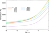 |
Fig. 2 Mean T(τ)-relations of the nine MHD simulations. |
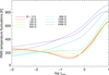 |
Fig. 3 Temperature fluctuations on surfaces of equal optical depth of the nine MHD simulations. |
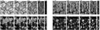 |
Fig. 4 Bolometric emergent intensity viewed at different limb angles for four MHD models with В = 0, 800,1600, 2400 G. For each model a selected snapshot is shown, ordered upper-left to lower-right. The gray scale is kept the same for each viewing angle of a particular snapshot. The increasing impact of the magnetic fields is apparent by the transition from quiet photosphere to sun-spot (umbral) conditions. |
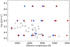 |
Fig. 5 32 HD models (red and blue dots) together with observational data (gray symbols) from M23 in the Teff-log ɡ-plane. Red indicates models of solar; blue models of 1/10 solar metallicity. The subset of systems also analyzed in M18 is depicted by gray squares. Most of the observed systems have slightly super-solar metallicity. One system with Teff < 4000 K is not shown. |
2.3 Calculation of spectral energy distributions and integration over the Kepler passband
For all 3D models we calculated spectral energy distributions (SEDs) that were subsequently integrated over the Kepler pass-band to obtain estimates of the observable fluxes. For the line absorption we took recourse to opacity distribution functions (ODFs) provided by Castelli & Kurucz (2003). We used the high-resolution “little” ODFs with 12 sub-bins. Continuum opacities were computed with the routines i ondi s and opal am, which are part of the 3D spectral synthesis code Linfor3D (Steffen et al. 2022; Gallagher et al. 2017). We restricted the calculations to wavelengths ≥ 133.5 nm (ODF bin 165) so that effectively 12,576 wavelength points were used to represent a SED. Table 2 lists the considered limb angles. For all models, limb angles according to the Lobatto scheme were available. Additional Gauss-Radau limb angles were only calculated for the MHD models. The reason for this choice was economic: the SEDs for the Lobatto angles had already been calculated for earlier investigations (Bonifacio et al. 2018; Kučinskas et al. 2018) and the extensive computations did not need to be repeated. A drawback is that the Lobatto angles do not cover positions close to the stellar limb. For that reason the subset of MHD models was augmented by the angles of a Gauss-Radau scheme. This particular choice was motivated by the fact that the Gauss-Radau angles fall in between the Lobatto angles and provide a point significantly closer to the stellar limb.
Figure 6 shows the resulting SEDs for various limb angles, µ, for the field-free model B0000. The given intensities are integrals over the 12 ODF sub-bins, expressed in terms of photon counts. One can discern the usual behavior that SEDs get fainter and redder as one moves toward the stellar limb. For comparison the transmission of the Kepler passband (Van Cleve et al. 2009) is shown, as well as the total transmission if we assume an interstellar extinction of AV = 1 mag using the extinction law of Cardelli et al. (1989); as expected, the extinction leads to a reddening of the throughput. An extinction of 1 mag is of course unrealistically high for the rather bright, close-by systems analyzed here. We chose this extreme value to get an impression of whether extinction might influence the analysis of the Kepler observations at all.
In the calculation of the SEDs, scattering opacities are treated as true absorption. This is perhaps the severest shortcoming for the accuracy of the synthetic photometry. The Kepler passband does not extend very far into the blue spectral range, where scattering is particularly important. However, especially close to the stellar limb – which is rather dark – contributions due to the scattering of photons from the brighter disk locations tangential to the line of sight may lead to some brightening.
Direction cosines of the two different ray configurations discussed in this paper.
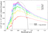 |
Fig. 6 Example (field-free model B0000) of the calculated intensity distribution, together with the Kepler passband. The reddening effect on the passband from interstellar extinction of 1 mag is depicted. Passbands are normalized to a maximum of one. Since Kepler effectively operates in photon-counting mode, intensities are expressed in terms of photon counts. |
2.4 Effects of sphericity
The 3D models of this investigation were built under the assumption of a planar, Cartesian geometry. In standard 1D model atmospheres this corresponds to the assumption of a plane-parallel symmetry. While often the planar geometry is an excellent approximation, it is clear that close to the stellar limb effects due to stellar sphericity render the approximation increasingly poor. For that reason we were seeking ways to account for sphericity effects without having to conduct 3D simulations in spherical geometry. Since for stars close to the main sequence the effects are rather mild, we devised a correction scheme with which we transformed the Cartesian intensity data to intensities obtained when taking the spherical geometry into account. The correction scheme works with the horizontally averaged (specifically temperature and geometrical height averaged over τross iso-surfaces) and temporally averaged 3D structures. For that reason we shall henceforth speak in terms of spherically symmetric and planeparallel structures, employing the nomenclature used in 1D stellar atmospheres.
2.4.1 Spherical correction of the 3D intensities
Figure 7 contrasts the actual spherical stellar geometry with the plane-parallel geometry assumed in planar 1D model atmospheres. A light ray in spherical geometry can be characterized by its impact parameter, b, which gives its (shortest) distance from the stellar center. Along a ray, the angle, θ, (green angles in Fig. 7) with respect to the radial direction changes as
 (6)
(6)
where r is the distance of the point of interest to the stellar center. In plane-parallel atmospheres, the angle, θ, is constant along a ray (blue arrow), and can thus serve as the label of a particular ray.
Figure 7 further illustrates what happens if one conceptually “flattens” a spherical geometry into a planar one. Rays (red arrows) that appear straight in spherical geometry appear more or less bent in planar space. The effect is in fact rather mild for the stars studied here (since the extent of the atmosphere is much smaller than the stellar radius) except for rays very close to the stellar limb. We altered a standard 1D radiative transfer code assuming plane-parallel geometry to take this slight “refraction” of rays according to Eq. (6) into account. It mimics radiative transfer in spherical geometry this way. As long as a ray belongs to the class of core rays, i.e., rays entering the optically thick part of the star, boundary conditions can remain unchanged. Only the mild change of θ needs to be accounted for. Besides being a rather simple procedure, this has the advantage that a clean differential comparison of the emergent intensities is possible in both geometries. We simplified the calculations by treating the problem in gray approximation using the Kirchhoff-Planck function integrated over the Kepler passband as source function, as well as gray Rosseland opacities. The simplification was dictated by a technical limitation of our 1D radiative transfer code that has not been written to work with ODFs. Appendix A gives an argument for why the Rosseland mean opacity is a reasonable choice and provides estimates of the accuracy of the gray approximation. We computed the intensity for given µ in planar and spherical geometry (see the following Sect. 2.4.2 for the association in both geometries), and used their ratio as a scaling factor for the full 3D intensity to approximately correct them for the effects of sphericity, viz.,
 (7)
(7)
This correction only becomes relevant for limb angles µ ≲ 0.05; the exact threshold depends on the atmospheric extension and targeted precision level. We emphasize that a clear-cut comparison between planar and spherical geometry, as needed for applying Eq. (7), is often not possible with stellar atmosphere codes since the radiative transfer is implemented very differently in both geometries. The mild effects present here are masked by the numerics.
For completeness, we add that relation (6) leads to a shape of ray in flattened, planar geometry given by
 (8)
(8)
(x, z) are Cartesian coordinates with the stellar center as origin. The ray geometry described by Eq. (8) preserves the relation (6) (substituting r → z) as well as the path length along the ray between z-levels. Unfortunately, the applicability of Eq. (8) is limited since in the context of model atmospheres one is usually interested in the function µ(z). However, we found Eq. (8) useful for plotting purposes.
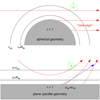 |
Fig. 7 Illustration of the ray geometry in spherical (upper half) and plane-parallel (lower half) symmetry. Gray regions correspond to the optically thick regions of the star. R⋆ is the stellar radius, z the vertical coordinate, and rtop the – somewhat arbitrary – uppermost level in the spherical or planar atmosphere. Red arrows depict how straight light rays in spherical geometry get bent when interpreted in planar geometry. The blue arrow depicts a ray in planar geometry. The yellow circle marks the location where the inclination angle of rays in both geometries coincides. The green angle illustrates the inclination angle of a ray with respect to the vertical. “Core rays” are rays that penetrate into the optically thick part of a star. |
2.4.2 The definition of the stellar radius
Before we discuss the intensity profile at the stellar limb, we here describe the definition of the stellar radius that we applied in this investigation. The stellar radius is attained where the limb intensity profile has an inflection point. This is a commonly adopted definition, in particular in observational work. We further assume a fixed solar radius of 696 Mm for all MHD models at the radius so defined. The radius value controls the magnitude of sphericity effects on the intensities at the Lobatto and Gauss-Radau limb angles, as well as the curvature at the extreme limb. According to Table 1 our definition formally implies that the radius of the optically thick core of the Sun slightly differs among the models. Whether this is actually the case depends on the effect of the magnetic field on the global stellar structure, and cannot be decided based upon the local models studied here.
When comparing intensities calculated under the assumption of planar or spherical geometry one has to decide how to associate rays among the geometries. In other words, we ask, which ray of particular µ in planar geometry does a ray in spherical geometry with impact parameter b correspond to? Since µ changes with height for a spherical ray, in planar geometry one has to decide about a reference depth where the spherical and planar angles coincide. We opted to set the zero point µ = 0 for a ray with b = R⋆. With this we have the simple association  . This means that R⋆ serves as the reference radius at which µ in the spherical and planar geometries coincide. This location is marked by a yellow circle in Fig. 7.
At this point the reader might wonder why we give a rather detailed motivation of our choice of the stellar radius and the related association between geometries. The reason is that in the literature there are conflicting conclusions about the relative importance of sphericity effects in FGK-dwarf stars (see, e.g., Neilson & Lester 2013) that we believe can be partly traced back to differing definitions of the stellar radius and the point where µ = 0. The choice of the position of the stellar radius has a strong impact on the functional dependence of I(µ) close to the limb (cf. Eq. (9)). Poorly adapted choices can enhance apparent differences between planar and spherical geometry.
2.4.3 Limb intensity profiles
For most models employed in this project, intensities calculated from time series of 3D structures are only available down to µ = 0.17 (for which a sphericity correction is unnecessary). However, to further characterize intensities encountered closer to the stellar limb without performing computationally demanding 3D radiative transfer calculations we again sought an approximate way to calculate them. The procedure and code described in Sect. 2.4.1 was only suitable for mildly spherical conditions. With “mildly spherical conditions” we refer to a situation where it is sufficient to consider rays that always reach into optically thick regions. Locations close to the stellar limb should not matter much for the atmospheric structure. To treat the strong sphericity effects near the stellar limb we followed a procedure laid out by Unsöld (1968). In short, he considers a plane-parallel atmosphere that is “bent” around a sphere – the considered star – of a given radius. In some sense one may consider this procedure as the inverse of the “flattening” of a spherical structure discussed in Sect. 2.4.1. In the now spherical geometry tangential rays are integrated through the structure, varying their impact parameter. Unsöld shows that for an isothermal atmosphere one has to expect an exponential drop in intensity with increasing projected radius (equivalent to the impact parameter). He defines the stellar radius as the position of the tangential ray that has an optical thickness of one along its path. The impact parameter of this ray corresponds to a radial optical depth of log τ ≈ −2.2. He emphasizes that this result sensitively depends on the pressure dependence of the opacity. Clearly, Unsöld’s geometrical transformation of a plane parallel into a spherical structure neglects any influence of the spherical geometry on the thermal profile of the atmosphere. However, we are considering stars close to the main-sequence for which sphericity effects on the photospheric thermal structure are not pronounced.
For each snapshot of a given 3D model we calculated the horizontally averaged atmospheric structure (specifically temperature and geometrical height averaged over τross iso-surfaces). We treated the snapshots separately to be able to quantify the statistical uncertainties of the derived limb intensity profiles. Working with the horizontal averages neglects the effects due to horizontal inhomogeneities. We expected that this generally has only a small effect since the tangential rays have a long path length. This leads to a large degree of cancellation of the effects related to the small-scale structural variations that a ray encounters along its way. However, as we will see, this only holds for models harboring not-too-strong fields. As in the case of deriving the spherical corrections to the 3D intensities, we worked with gray Rosseland opacities and the Kirchhoff-Planck function integrated over the Kepler passband as the source function (computed from the local temperature).
Figure 8 illustrates the outcome of the approach described above. Solid lines show the results of the fitting procedure to 3D data, as explained in a later section. The dashed lines depict the limb intensities of the MHD models calculated using their averaged (ID) structures, applying the gray approximation. For the unit of intensity, we used the flux, as calculated from the fitted LD law divided by π – i.e., the mean disk brightness. Consequently, the unit of intensity differs among the models. We opted to use a semi-logarithmic plot, which is motivated by Unsöld’s result of an approximately exponential drop-off in intensity at the limb. Indeed, the calculated drop-offs almost follow straight lines, indicating that in the case of realistic temperature stratifications, too, the drop-offs are close to exponential. Dots at the right end of the solid curves mark the abscissa where the inflection point (not evident in the linear-log representation) of the intensity profile is located. This defines where the stellar radius is attained (see Sect. 2.4.2). Table 1 lists their optical depths, 1g τ⋆. We see that the optical depth of this point varies only slightly among the models, and is ≈0.2dex smaller than Unsöld’s estimate; however, in view of Unsöld’s approximations the correspondence is quite satisfactory. The dot to the left on the solid curves is located at μ = 0.04; its relevance is explained in Sect. 2.5.2.
Figure 9 compares intensities obtained for ID planar and spherical geometry in the gray approximation. It is obtained as a combination of what was previously described as the calculation of a spherical correction and limb profile. The model of lower gravity shows larger differences between the geometries as expected, by scaling with relative atmospheric extension, HP/R⋆, where HP is the pressure scale height at the stellar surface. As stated before, the differences get noticeable for μ ≲ 0.05. However, this part of the CLV curve leaves hardly any detectable imprint in the transit light curves of hot Jupiters, and thus is not particularly relevant in the observational analysis. To relate the geometrical coordinate z used in Fig. 8 to the µ-scale in Fig. 9, the following relation from a Taylor expansion valid for small, positive μ might be helpful:
 (9)
(9)
z⋆ is the height at which the stellar radius is located – see Table 1. As is evident from the table, z⋆ roughly drops with increasing field strength. The optical depth at z⋆ remains largely invariant.
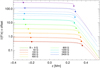 |
Fig. 8 Intensity proflies at the extreme stellar limb of the nine MHD models. The solid lines are the fitted intensity profiles using the Claret-4 law. The dashed lines depict the result of radiative transfer calculations along tangential rays in the gray approximation. The dots to the right mark the position μ = 0 (the location of the stellar radius), and the dots to the left μ = 0.04. The solid lines end at dots marking μ = 0 as the stellar limb and limit of definition of the Claret–4 law. For clarity, the curves were scaled in steps of factors of two in the vertical direction, with model В = 0 G at its original position. In this plot, the zero points of the z-scales are located at a radial Rosseland optical depth of one in the respective model. |
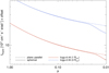 |
Fig. 9 Comparison of intensities in the Kepler passband calculated in spherical and plane-parallel symmetry. The results are shown for two models of approximately solar effective temperature and metallicity but different surface gravity. For clarity, the intensities of the log ɡ = 3.5 model were scaled by a factor of two. The intensities were calculated in the gray approximation. |
2.5 Fitting the synthetic intensity data and regularization of the fits
2.5.1 Temporal fluctuations of the spatial Intensity profiles
The convectively driven surface flows exhibit a deterministically chaotic character. As such, a flow simulation can be considered as a Monte Carlo experiment and the results are subject to statistical uncertainties that can be quantified by the temporal variability of the features of interest. For each MHD model, 20 statistically independent snapshots were selected. Figure 10 illustrates the temporal fluctuations of the intensities as a function of the limb position. Intensities belonging to the same instance in time are fitted with a Claret-6 law to guide the eye. At this stage in the fitting process, all points except at the very limb were weighted equally and were considered uncorrelated. Since the snapshots are statistically independent we expect that the achievable precision of the temporal mean of a feature scales inversely with the square-root of averaged instances. In the plot some general properties are discernable: (i) with increasing field strength temporal variations increase , which can also be expected from the increasing temperature fluctuations with field strength as shown in Fig. 3; this is apparent from the area covered by the individual profiles of a model in the plot; (ii) spatially, the intensities are highly correlated, and temporal variations appear as “up-down wobbling” of the profiles in the plot. The wobble is driven by variations in the effective temperature from snapshot to snapshot. In the case of the highly variable model B2400, RMS fluctuations in Teff amount to ≈ 100 K, with a peak-to-peak variation of ≈ 440 K. Lacking models of different Teff at 2400 G, we took the variation in the shape of the CLV curves with Teff among the field-free models as indicative for variability at 2400 G. We found that the Teff fluctuations present in model B2400 cannot alter the shape of the CLV curve to a degree that renders them qualitatively different among the snapshots. We used the temporal fluctuations to calculate the full covariance matrix of the temporal mean intensity profile for each model. As is discussed below, the inclusion of the full covariance matrix when fitting the temporally averaged intensity profile caused problems that ultimately led us to ignore correlations among the uncertainties at different limb positions.
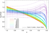 |
Fig. 10 Time-resolved synthetic intensities of the nine MHD models (open circles) fitted with the Claret-6 law (solid lines; color encodes the model) to guide the eye. Intensities are given in units of the temporal average of the mean surface brightness of each model; that is, the unit of intensity is temporally fixed for each model but differs among them. No corrections for sphericity effects were applied. |
2.5.2 Fitting the synthetic 3D intensities
For the field-free models, only synthetic intensities at the limb angles of the Lobatto scheme (see Table 2) were available. Besides providing a rather coarse discretization this also meant that data points close to the limb were missing. To obtain a smooth representation of the synthetic intensities over the whole range, µ ∈ [0,1], we decided to fit the synthetic intensities with a Claret-4 law – or a Claret-6 law in the case of MHD models for which additional intensities according to the Gauss-Radau scheme were available. The fits provided a handy analytical form of the intensities derived from the 3D simulations. To solve the maximum likelihood problem we applied the LevenbergMarquardt algorithm, as implemented in the IDL package mpfit by C.B. Markwardt (Moré 1978; Markwardt 2009).
Two major obstacles needed to be addressed in the fitting. Initially, we intended to include the full covariance matrix of the uncertainties of the synthetic intensities in the fits (making use of the routine mpfitcovar). This resulted in implausible fits; we put this down to the basic reason that neither the Claret-4 law nor the Claret-6 one are true generative models of the intensity data – in the present context simply meaning that their functional forms cannot provide a perfect match to given noise-free intensities of the physical model irrespective of the chosen LDCs. Apparently, little attention is paid in the statistical literature to this problem, and we did not find a suitable reference. For that reason we give a detailed, analytically tractable example in Appendix E illustrating the problem. As a practical consequence, we neglected the correlation among the uncertainties of the intensities in the fitting. We emphasize that this is a conservative choice in the sense that this increases the volume of the confidence region of the fitted parameters. Nevertheless, even so we obtained fits of the coefficients of the LD laws of sufficient precision.
Neglecting correlations resulted in reasonable fits to the data points, however, the extrapolation of the 3D intensities toward the limb µ → 0 using the LD law often gave unphysical behaviors; one obtained negative intensities at µ = 0, or implausible, strong increases in the intensity toward the limb. To regularize the fits close to the limb, we used the limb intensities that we calculated previously (see Sect. 2.4.3). We tried to constrain as little as possible, in particular not using the calculated intensities proper, since they were obtained from the mean stratification in the gray approximation. By trial and error we found that it was sufficient to constrain the fits by specifying the intensity ratio between µ = 0 and µ = 0.04. Considering a ratio lets the various approximations entering the calculation of the intensity profile at the stellar limb be less critical. The extent in depth of a mean 3D model placed (conceptionally) at the stellar limb sets a limit to the minimum impact parameter or equivalently maximum µ-value of a tangential ray that can pass through the model. The location µ = 0.04 was the maximum that all 3D models could accommodate. Besides considering intensity ratios only, to be even less constraining we artificially increased the formal uncertainty of the ratios by a factor of ten. We emphasize that the regularization was also necessary when fitting the Claret-6 law. In particular, the intensity at µ = 0.057 was not sufficient to always enforce reasonable behavior in the vicinity of the limb.
Figure 8 shows a comparison of the fitted Claret-4 law and the limb intensity profile for the MHD models. The MHD models are a good test suite since their LD curves show a variation greater than what is seen among all field-free models. It is remarkable that the Claret-4 law can reproduce the intensity ratios as suggested by the limb intensity profiles (dashed lines in Fig. 8). The correspondence with the absolute intensities varies: at field strengths B ≤ 800 G it is rather good, whereas at larger field strengths the extrapolation of the fitted LD law predicts systematically higher intensities than suggested by the limb profiles. This behavior can be explained by horizontal inhomogeneity of the MHD models that is neglected in the horizontally (and temporally) averaged structures underlying the limb profiles. Figure 4 shows that magnetic features lead to a brightening at the limb, since they have a certain extent in height and exhibit bright “walls”. The limb intensity profiles do not include this effect. Hence, we do not consider the mismatch in absolute intensity between extrapolated LD law and limb intensity profile worrisome, and moreover consider the extrapolated intensity as more realistic since it is based on a full 3D treatment, including the structural effects of magnetic features.
Figure 11 compares fits of the Claret-4 law to the intensity data of the MHD models when using five intensity points, as provided by the Lobatto scheme, and nine intensity points when combining Lobatto and Gauss-Radau points. The synthetic intensities were corrected for sphericity effects according to Eq. (7). The apparent difference among data points for the same model and the same µ comes about by a slight difference in the flux attributed to a model; fluxes differ since the discrete flux integral depends on the chosen limb angles and integration weights, which in turn differ between five or nine data points. All fits represent the intensity data reasonably well. The behavior of all models close to the limb appears plausible. Interestingly, the two models with the strongest field show regions with dI/dµ < 0. This is not found in field-free models. All models share an approximate fix point at (µ ≈ 0.6,I/(F/π) ≈ 1). We interpret this as a consequence of the Eddington-Barbier relation, which states that approximately
 (10)
(10)
holds. S is the source function. F, S, and I should be interpreted as integrals over the Kepler passband. For τ, the Rosseland optical depth may be taken (see also Appendix A). The smooth dependence of the source function on the optical depth of the MHD models as implied by Fig. 2 makes it plausible that all LD laws pass close to the point (µ = 2/3, I/(F/π) = 1), so that the presence of the fix point is not surprising. Finally, the fitted LD curves applying five or nine data points look almost identical at small field strengths. This is important, since it implies that the LD curves for all field-free models can be reliably obtained from the five available angles of the Lobatto scheme. We verified that switching between five and nine limb angles for the MHD models does not substantially alter the comparison with the observations. Since we used nine angles in the comparison we consider the associated results to be robust. All intensity data underlying the fitted LD curves are listed in Appendix H.
2.5.3 Light curve generation and like-for-like comparison
Following Howarth (2011), M18 emphasizes the importance of comparing observations and theoretical predictions on an equal footing - something Howarth called performing a “like-for-like” comparison. To calculate a particular LD coefficient (like h′1) one could take recourse to a calculated LD curve directly (here typically represented by a Claret-4 law), applying its definition; in the following we call this a “direct calculation”. However, observationally, a derived LD profile is the result of a fit to a measured light curve. The fit depends on the chosen LD law, transit geometry, and weighting of the various phases of the transit. M18 used the power-2 law as the LD model in his analysis. We replicate the observational procedure here by using the calculated LD curves based on the Claret-4 law together with the derived transit geometry to synthesize a light curve. Thereafter we fitted this light curve with a light curve calculated with a power-2 law to obtain like-for-like LD coefficients. As detailed in Appendix C, we introduced a number of simplifications in the generation of light curves, which, however, we show to be immaterial on the precision level aimed for in this investigation. An important benefit of the simplified light curve generation was speed: it allowed us to run hundreds of light curve fits in an interactive fashion.
In a like-for-like determination the LDCs of a particular system depend on six parameters, (p, B), where we introduced the parameter vector p ≡ (Teff, log ɡ, [Fe/H], b, k) for brevity. b is the impact parameter of the transit (see also Fig. C.1), k the planetary radius, both in units of the stellar radius. Except for the magnetic field strength, B, all other parameters were obtained in the analysis of the system. In order to calculate the LDCs for a particular system we took recourse to our 32 non-magnetic 3D models. For each model we generated a light curve for the given transit parameters (b, k), assuming B = 0 (since applying field-free 3D models). Thereafter, we performed polynomial fits to h′1 and h′2 in (Teff, log ɡ, [Fe/H]) space, which we used to evaluate the LDCs of the system for the observed atmospheric parameters of the system. We did not conduct an interpolation since we do not consider our results of the simulations to be exact but subject to statistical uncertainties. A certain degree of smoothing of the modeling results is provided by a fit and hence appears advantageous.
Figure 12 depicts one example of a polynomial fit for transit parameters b = 0 and k = 0.1 in the h′1-h′2-plane. We used 16 terms in the fits of h′1 and h′2, up to third order in Teff, quadratic in log ɡ, and linear in [Fe/H]. The 1σ joint confidence regions were obtained by propagating the uncertainties of the LDCs of the Claret-4 LD curves through the light curve fitting procedure. One can discern that the polynomial fit is compatible with but not perfectly representative of the model data. This reflects the – to some degree arbitrary – choice of the functional form of the polynomial. However, we experimented with various forms and found that the given form is a good compromise between simplicity, precision, and representing the essential features. To further validate the basic morphology of the fit, we performed a Gaussian process regression, which recovered the structure displayed in Fig. 12 as well. Most importantly, we find for Teff ≳ 5500 K a clear sensitivity of the LDCs on log ɡ. For smaller Teff and log ɡ ≳ 4.0 the sensitivity is significantly lower.
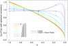 |
Fig. 11 Time-averaged synthetic intensities of the nine MHD models fitted with a Claret-4 law. Filled circles and solid lines depict the result for the Lobatto angles; open circles and dash-dotted lines the result when Gauss-Radau angles are added. Intensities are given in units of the mean surface brightness of each model. Corrections for sphericity effects were applied. For further details, see the text. |
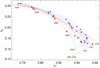 |
Fig. 12 Example of polynomial fits in stellar parameter space to h′1 and h′2 from light curve analyses for transit parameters b = 0 and k = 0.1. Red dots with 1σ joint confidence regions depict the results of 3D models of solar metallicity, and blue dots the results for metallicity [Fe/H] = −1. Lines of constant Teff and log ɡ are added to illustrate the functional dependence. Line segments connect data points and corresponding values predicted by the polynomial. |
2.5.4 Normalization of the observational data
Since our MHD models are limited to solar conditions only, an immediate comparison to systems with non-solar atmospheric parameters harboring magnetic fields is not possible. To at least partially circumvent this limitation we came up with the idea of comparing the difference between observed and calculated LDCs based on the polynomial fit described in the previous section; these differences we added to the LDCs of a standardized transit, for which we assumed a host star with solar atmospheric parameters and a transit with b = 0 and k = 0.1. The resulting normalized LDCs can be formally written as
 (11)
(11)
with ![Mathematical equation: ${{\bf{p}}^ \odot } \equiv \left( {T_{{\rm{eff}}}^ \odot ,{\rm{log}}\,{g^ \odot },{{\left[ {{{{\rm{Fe}}} \mathord{\left/ {\vphantom {{{\rm{Fe}}} {\rm{H}}}} \right. \kern-\nulldelimiterspace} {\rm{H}}}} \right]}^ \odot },\,b = 0,k = 0.1} \right)$](/articles/aa/full_html/2023/11/aa46783-23/aa46783-23-eq14.png) . “obs” indicates observed values, “cal” calculated values from a polynomial fit, and “norm” the normalized, final values. The fundamental assumption underlying this approach is that all host stars are not too different from the Sun. As a consequence, the effect of a magnetic field in a host star is essentially the same as that present in the Sun. This is a strong assumption, for which some justification is provided later.
. “obs” indicates observed values, “cal” calculated values from a polynomial fit, and “norm” the normalized, final values. The fundamental assumption underlying this approach is that all host stars are not too different from the Sun. As a consequence, the effect of a magnetic field in a host star is essentially the same as that present in the Sun. This is a strong assumption, for which some justification is provided later.
3 Results
3.1 Comparing (h′1, h′2) of the MHD models with observations
Figure 13 provides an overview of the behavior of the CLV of the MHD models in the h′1 -h′2-plane together with observational data from M18. For each MHD model three different values are depicted: filled colored squares indicate the LDCs (h′1, h′2) from the light curve fitting, filled colored circles the values normalized to solar conditions, and filled diamonds the result of the direct calculation based on the underlying Claret-4 law. In the case of the MHD models, the normalization procedure corrects for their differing effective temperatures only since all other parameters, including the assumed transit geometry, correspond to solar standard conditions. We fitted the normalized MHD data by a cubic function in B (solid black line with labels) to guide the eye; in the fitting we left out the B2400 model (violet symbols) since its inclusion led to a significantly worse overall representation of the MHD data, especially at small field strength. The LDCs derived from observations by M18 are depicted by open black squares, and their normalized values by filled gray circles; the original and normalized positions are connected by a line. As evident from the vectors indicating the sensitivity to atmospheric parameters (evaluated at the solar position), the normalization mostly corrects for the Teff offset between an observed star and solar Teff. In essence, all normalized data points depicted by filled dots – be they from observations or models – should correspond to host stars with solar atmospheric parameters that only differ in their level and morphology of magnetic activity. That allows for a direct comparison between them.
One important aspect of the normalization is its tendency to make the observational data form a one-dimensional sequence – presumably with the magnetic field strength as a controlling parameter – lying to the lower right of the solar position. We took this tendency to order the observations in the direction of increasing magnetic activity as an indication that our normalization procedure is indeed meaningful.
Colored filled squares and filled diamonds mark the results for a direct and like-for-like calculation, respectively. Differences between both ways of calculation become larger at higher field strengths. However, these differences are not decisive for our comparison.
We found an offset between the position of the B0000 model and the solar locus, as predicted by the 32 field-free models. The MHD models are not fully consistent with the non-magnetic models underlying the polynomial fit used in the prediction. We checked various possibilities as to why this is the case. We initially suspected that the different diffusivities of the applied hydrodynamics solvers (HLL vs. Roe for the magnetic and nonmagnetic models, respectively) affect the model structures. We ran a dedicated field-free test model using the Roe solver but otherwise being identical to model B0000. It turned out that the choice of the hydrodynamics solver does not matter, as the LD came out almost identical. Further tests showed that the number of opacity bins used in the model runs had a mild impact on the CLV of a model. Unexpectedly, it turned out that the biggest impact had the radiative transfer solver applied when calculating the SEDs of the hydrodynamical models. The SEDs of the HD models were calculated with a significantly older version of our radiative transfer code. In the meantime a new solver was implemented. We now consider the normalized position of our B0000 model the “best guess” calculation of a field-free star with solar atmospheric parameters. We corrected the small offset between the normalized model B0000 and the solar location as predicted by the polynomial fit to the field-free models by applying a global shift of ∆(h′1, h′2) = (+0.00900, −0.00843) in the normalization of all observational data.
The dashed line in Fig. 13 depicts the result of an additive mixing (see Appendix D) of models B0050 and B1600; the surface area fraction attributed to model B1600 is given by the percent labels along this “mixing line.” The line is intended to illustrate what may happen if spot-like magnetic fields and quiet photospheric conditions were present simultaneously on the stellar surface; we also hoped to obtain a closer match to Kepler-17. We chose the two models for being representative of the actual Sun (the 50 G we took as representative of what to be expected from its small-scale dynamo) and a spot that is not fully developed. We would have preferred to use the B = 2400 G model; however, during the normalization of all the intermediate, mixed models we ran into cases with fitting problems. Since the mixing line came out as an almost straight cord we did not expect that it would make much of a difference as far as its location is concerned. One just had to expect a smaller surface area fraction, which is needed for obtaining a particular (h′1, h′2) position. In any case, one can note that mixing areas of different field strength is not the same as covering the whole of the same surface by the corresponding mean field.
Here, we note an important aspect of our construction: the fact that our MHD models share the same entropy value in their deep layers lets our mixing line appear to be a possible physical model. If entropies were different one would expect strong currents in the deep layers that would try to equalize the entropies. This would make a side-by-side arrangement of model patches with different field strengths highly unstable.
Figure 14 is a zoom-in on Fig. 13 with a focus on the observational data. It is different from Fig. 13, as only the normalized observational data points are plotted. Our “best-guess” field-free Sun is marked by the solar symbol. The 1σ joint confidence regions of the observational data are depicted as well, illustrating the still sizable observational uncertainties1. Figure 14 summarizes the most important results of this investigation. Without observational errors and after normalization, all observational data points should fall on the solar position – provided magnetic activity is not present. It is remarkable that observational data points occupy a region to the lower right of the solar position. When looking at the MHD models, a shift to the right is expected if magnetic fields influence the CLV. Obviously, perfectly homogeneous conditions do not provide an adequate match since all observations fall below the line defined by the MHD models in the h′1-h′2-plane. Moreover, to explain some shifts to the right, field strengths in excess of 100 G were necessary; such strengths of the vertical component of the field around optical depth unity are not to be expected if small scale dynamo action in the surface layers is the driving agent (Bhatia et al. 2022; Witzke et al. 2023; Riva et al. 2023). Small scale dynamo action appears to be an attractive option if one is looking for a mode of magnetic activity that operates homogeneously across the stellar surface. Alternatively, the mixing line more closely traverses the region occupied by the observational data points. While the match is not perfect either, we take this as an indication that a “salt and pepper”-like combination of stellar spots and nearly field-free regions are a more likely morphology of the surface fields. The tendency of the observations to lie below the mixing line points toward lower h′2- and/or h′1-values than predicted. This in turn means that the stellar limb appears brighter in the observations than in our MHD models.
In this context, Kepler-17 is a key object; the star is known to be magnetically fairly active, and was the target of a number of detailed investigations of its spot distribution (e.g., Valio et al. 2017; Lanza et al. 2019). Lanza and collaborators derived an average spot-filling factor of about 7%, assuming an intensity contrast between the spot and the quiet photosphere of 0.55. While we do not obtain a good fit to Kepler-17, our mixing line would rather indicate a filling factor in the range of 20… 30% at a spot contrast of 0.63 at the disk center (approaching and exceeding one closer to the limb, see Fig. G.2), and hence, the quantitative correspondence is not good. However, one has to keep in mind that the value of Lanza and collaborators is a longitudinal average, while our spot coverage refers to the surface strip occulted by the planet during its transit. The transit of Kepler-17b happens close to the stellar equator that may potentially be more active than higher latitudes. Moreover, we calculated the mixing line using the B1600 model to be representative of spots. It is well possible that typical field strengths in spots are higher than assumed in this model. Higher field strengths in spots would enhance the spot contrast so that a smaller spot-filling factor would be sufficient to fit Kepler-17. However, while the aforementioned effects reduce the gap between observation and theoretical prediction we doubt that they can fully explain the discrepancy. A fully convincing explanation still needs to be found.
For completeness, we also investigated the more recent observational data of M23. Unfortunately, we find that they add little new information so we do not discuss these results here further. Appendix F provides details.
We did not obtain a convincing fit of the observational data of M18 with our models. However, our normalization procedure led to a roughly one-dimensional sequence of the observational data. We intended to emphasize this fact while refraining from attributing a particular field strength to an observational datum. To this end, we used the distance between a data point and the solar position to rank the observations according to field strength. Table 3 lists the result. A distance, s, was simply calculated as the geometrical distance between an observational datum and the solar position according to  (the formula for s given in Table 3 is equivalent). Since the RMS dispersion of h′1 and h′2 among the observations is similar, we decided to leave out any weighting of their contributions. We used Gaussian error propagation of the observational uncertainties (including correlations) to calculate the 1σ uncertainty of s, σs. As is already evident from Fig. 14, a few observations are compatible with field-free conditions. The sometimes substantial uncertainties imply a certain degree of blurring of the ranking, meaning that some shuffling of the order is possible. The list should nevertheless allow one to correlate the quantity, s – as a proxy of the magnetic field strength – with newly measured parameters presumably also affected by magnetic fields. We in fact searched for such correlations with orbital characteristics of the systems and found a tendency of systems with planets of larger relative radius, k, to show higher field strengths. However, since the total number of systems is small and we do not see a physical reason why this should be the case, we consider this to be a correlation by chance.
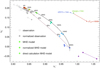 |
Fig. 13 Comparison between observations of M18 and calculations in the h′1-h′2-plane. Symbols in color depict the results from solar MHD simulations. Gray and black symbols show the observational data. Data points before and after normalization are connected by a line. The solid black line labeled with field strengths is a fit to the MHD models to guide the eye. The dash-dotted line illustrates the outcome of an additive mixing of models B0050 and B1600, where percentages give the area fraction contributed by B1600. See the text for more explanations on the approach. The colored arrows indicate the sensitivity of the (h′1, h′2)-vector to the atmospheric parameters. |
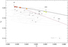 |
Fig. 14 Like Fig. 13 but zoomed in on the region with the observational data. The ellipses show their 1σ joint confidence regions. The best-guess solar position as obtained from model B0000 after normalization is marked by the solar symbol. |
3.2 Effect of interstellar extinction
While we did not expect extinction to have a significant impact on the analyses of M18 and M23, we nevertheless wanted to get an idea of its potential effect. To this end, we calculated LDCs assuming the extinction law given by Cardelli et al. (1989) with a rather strong extinction of AV = 1 mag. In Fig. 6, we have already shown the resulting change of the effective passband. Figure 15 compares the reddened and reddening-free case for (h′1, h′2). It turns out that the differences are surprisingly small and largest at small field strengths, which is the region we focus on in the plot. Not shown are models of higher field strengths where the differences get even smaller, almost vanishing at 1600 G. In the Kepler passband, extinction is almost perfectly degenerate with an increase in the strength of a homogeneous field (see tick marks along the fitted curves in Fig. 15). While a field configuration of covering the whole stellar surface homogeneously is certainly not realistic, we nevertheless expect that it would be difficult to disentangle the effect of magnetic fields and strong extinction. Spectral information would certainly help to lift this degeneracy.
Approximate ranking of the systems analyzed by M18 in order of increasing field strength.
3.3 Impact on interferometric measurements of stellar radii
When deriving stellar radii in terms of their apparent angular diameters, ϕ, from interferometry one has to account for effects of LD. Hestroffer (1997) provides an approximate relation (here expressed using α as a dimensionless auxiliary quantity),
 (12)
(12)
for the necessary correction factor. ϕLD denotes the limb darkened diameter and ϕUD the diameter derived for a uniformly bright disk. He obtained the factor given in Eq. (12) assuming a simple LD law of the form (expressed using our notation)
 (13)
(13)
We described our results in terms of LDCs (h′1, h′2). To associate this with the LD law of Eq. (13) we required that the disk center intensity and intensity at µ = 1/3 should be the same, giving the same (h′1, h′2) with the law given by Eq. (13). The two points appear suitable to establish a similar shape, putting weight to the regions close to the limb. The choice results in a relation,
 (14)
(14)
We define the relative change of the stellar diameter when considering models with B ≠ 0 relative to the field-free case as
 (15)
(15)
In Table 1, we list ∆ϕifr calculated from (h′1, h′2) of the normalized MHD models (see also Fig. 13), meaning that the values refer to a star with solar atmospheric parameters. The result for B2400 is missing, since α of the model is smaller than zero and thus falls outside the validity range of the approximation given by Eq. (12). We have seen that with an increasing magnetic field the stellar limb gets brighter, i.e., the LD is reduced, making the brightness distribution of the stellar disk look more uniform. Interpreting interferometric measurements with strongly limb-darkened field-free models leads to an overestimation of the stellar radius if the star harbors a magnetic field. However, the effect is small, and one would need fields with ≳300 G homogeneously covering the star for a radius reduction of ≳1%. At least small-scale dynamo action is likely not capable of producing such fields in solar-like stars (Bhatia et al. 2022; Witzke et al. 2023; Riva et al. 2023). We remind the reader that in this section we refer to – somewhat artificial – visibilities measured in the Kepler passband.
Kervella et al. (2017) performed diameter measurements of the components A and B of the α Centauri system with the VLTI/PIONIER interferometer in the near-infrared H-band. They could measure visibilities beyond the first lobe, which enabled them to constrain the CLV of the stars. They found that a LD law according to Eq. (13) can fit the observed visibilities well, and concluded that predictions from model atmospheres (1D as well as 3D) overestimate the degree of LD on a level, leading to an overestimation of the stellar radius by 0.5%. According to our results, the findings of Kervella and collaborators may indicate the presence of magnetic fields on the surfaces of the two stars. However, we cannot perform a quantitative comparison, since the measurements were taken in the H-band for which we expect significant differences to the LD in the Kepler passband. We nevertheless find the qualitative correspondence between MHD models and interferometric measurements encouraging.
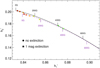 |
Fig. 15 Effect of extinction: filled circles depict the standard LDCs (h′1, h′2) without interstellar extinction; filled stars depict them when assuming an extinction of AV = 1 mag. All data are normalized to solar conditions. The solid black line with labels is a fit to the reddening-free data points; the dashed violet line to the reddened ones. The coloring of the symbols according to field strength follows our standard color scheme. |
4 Summary, conclusions, and final remarks
The most important result of this investigation is that the inclusion of magnetic fields in 3D simulations of surface convection brings spectral synthesis calculations of the center-to-limb variation in solar-like stars closer to observation. The MHD simulations predict that magnetic activity leads to a relative brightening of regions close to the stellar limb, which reduces the overall degree of LD. Magnetic fields make the mean temperature gradient in the deep photosphere shallower. In addition, magnetic features produce a hot wall effect that leads to a significant brightening at the stellar limb. Quantitatively, the correspondence between synthetic and observed CLV is not perfect (see Fig. 14), and further investigations are necessary to clarify the reasons for the mismatch. The perhaps most obvious shortcoming on the theoretical side lies in the assumption of a homogeneous field at large spatial scales when it is more likely that the stellar field is organized in spots and active regions embedded in quiet areas in which only a small-scale local dynamo is operational. Moreover, the 3D models of different field strengths can be interpreted as surface patches of various degrees of magnetic activity. They are not complete stellar spots. Among other things, that means that the Wilson depression expected for spots is not present, which may have an effect, especially with regard to structures close to the stellar limb.
In our pilot study, models of rather low spatial resolution were used, and we mainly investigated a field configuration that is forced to be vertical at the top and bottom boundaries of the computational domain. The maximum considered field strength of 2400 G is perhaps also a limitation, and higher field strengths should be considered. Last but not least, our simulations were done for conditions encountered in the Sun. We tried to mitigate the consequences of this restriction; however, the necessary approximations might not be as good as hoped for, so an extension of the modeling efforts to more spectral types is desirable.
Direct spectral synthesis calculations for the Kepler passband were conducted down to limb angles µ ≈ 0.05 only, leading to problems when fitting LD laws. We overcame this problem by deriving approximate limb intensity profiles, which we used to regularize the fits. LD laws are a data product of interest in the PLATO satellite project. The PLATO consortium recommends a set of limb angles with the smallest value µ ≈ 0.0l (Morello et al. 2022). Including such small angles in the fits may make a separate consideration of limb intensity profiles unnecessary but created a demand for 3D spectral syntheses, including sphericity effects.
We put substantial effort into modeling the intensity profile at the stellar limb. It turned out that for the modeling of light curves this was not particularly important, since the immediate limb region is difficult to access observationally. The derived limb intensity profile played only a role in regularizing fits of the Claret-4 or Claret-6 LD laws to the synthetic intensity data. The lack of an analytical form that can represent intensities from the disk center to and including the limb was a significant obstacle to making rapid progress. New ideas in this direction would be helpful.
The modeling of the limb intensity profiles was based on horizontally (and temporally) averaged 3D structures only. It turned out that the limb brightening seen at high field strengths using the full 3D models is caused by corrugations produced by magnetic structures and is not captured by working with averaged 3D models. This needs to be kept in mind when calculating intensity profiles close to the stellar limb.
We showed that interstellar extinction at a level AV ≲ 1 mag has little effect on the CLV in the Kepler passband, and is largely degenerate with the magnetic field strength. This means that both processes are hard to disentangle observationally – at least as long as only a single passband is observed. Similarly, interferometric radius measurements are little (≲1% relative change) affected by magnetic fields as long as a global field strength remains below ≲300 G; again, this statement refers to broad band measurements at optical wavelengths similar to what is provided by Kepler.
On the observational side, investigations of magnetic fields in late-type stars would benefit from more high-quality observational CLV data, especially extending measurements to very active stars. Since many transits need to be averaged to achieve the necessary precision, we will likely have to await results from the PLATO mission. Moreover, spectral information on transits would also be helpful. JWST appears particularly promising here for delivering outstanding spectral coverage of transit events.
The more recent results of M23 generally provided very uncertain LDCs compared to the earlier values in M18. This was caused by a change in methodology when fitting the observed light curves. Each analysis method comes with its specific systematic biases and it is not easy to judge which provides results of higher accuracy. In any case, in analyses one should keep in mind that the effects of magnetic fields will only be discernable at the highest achievable precision.
All in all, it remains interesting to see that the CLV in late-type stars indeed carries information on magnetic surface activity. High-precision photometry missions will continue to allow the exploitation of this window into stellar activity.
Acknowledgements
The authors thank Pierre Maxted for providing the observational data on h′1, h′2, and h2pp for his 2018 analysis. We further thank Daniel Reese for insightful discussions on correlated uncertainties. Figure E.2 was inspired by a similar plot created by him. The CO5BOLD MHD simulations were carried out on the compute cluster of the Leibniz Institute for Astrophysics Potsdam (AIP). H.G.L. acknowledges financial support by the Deutsche Forschungsgemeinschaft (DFG, German Research Foundation) – Project-ID 138713538 – SFB 881 (“The Milky Way System”, subproject A04).
Appendix A The Rosseland mean opacity as a suitable opacity average for calculating passband-integrated emergent intensities
To calculate the intensity at the stellar limb, or to derive the spherical correction factors, the mean stratification of the 3D models was used. The mean stratifications were calculated by temporal and horizontal averaging of the full 3D structures on surfaces of equal optical depth. To obtain the intensity integrated over the Kepler passband, one should first compute the detailed wavelength-dependent radiation field and afterward integrate over the Kepler passband, taking into account the transmission, 𝒯 (λ). The emergent intensity of a semi-infinite atmosphere along a line of sight can be written as
 (A.1)
(A.1)
For reasons of computational economy, it is desirable to replace the integrals over τλ by an integral using a suitably chosen mean τ-scale,  so that one can interchange the integrals over the wavelength and the optical depth:
 (A.2)
(A.2)
SX is the source function integrated over the Kepler passband, X. The central question is which  to choose in order to minimize the error made by replacing the integrals over τλ by a single integral over
  . In the following we show that the Rosseland mean opacity and associated τ scale are a reasonable choice.
We make the following assumptions:
the emergent monochromatic intensity can be approximated via the Eddington-Barbier relation as Iλ(τλ = 0) ≈ Sλ (τλ = 1)
 and any monochromatic opacity, κλ show small variations along the line of sight
With these assumptions we obtain for the relations between monochromatic τλ-scales and mean  -scale
 (A.3)
(A.3)
In the spirit of the Eddington-Barbier relation it appears natural to demand that the emergent intensity, ΙX integrated over the Kepler passband emerges from a mean optical depth,  = 1. This is because the Eddington-Barbier relation is an exact solution of the radiative transfer equation for a linear dependence of the source function on optical depth.
From now on we assume that the source function is given by the Kirchhoff-Planck function, Βλ. We approximately relate Βλ(τλ) and Bλ( ) by a first-order Taylor expansion around
  , viz.
 (A.4)
(A.4)
With this we can express the emergent intensity, ΙX integrated over the Kepler passband as

 (A.5)
(A.5)
with T denoting temperature (not transmission). The second term in the equation above is a correction term, the influence of which we want to minimize by choosing  so that it becomes zero. From that, it follows immediately that
 (A.6)
(A.6)
This is the Rosseland mean opacity calculated over the Kepler passband. Since the Kepler passband is rather broad we ignored this fact and used global Rosseland averages calculated over the whole wavelength range.
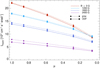 |
Fig. A.1 Comparison of emergent intensities in the Kepler passband calculated using wavelength-independent Rosseland opacities (“gray”), and wavelength-dependent opacities based on opacity distribution functions (“ODF”). The results for the four mean structures of MHD models are depicted assuming plane-parallel symmetry. |
We performed test calculations to estimate the accuracy of the gray approximation. For the horizontal-temporal mean structures of the nine MHD models we computed the intensities in the Kepler passband, once using ODFs and once using gray Rosseland opacities as described above. Since our code for calculating spectral energy distributions with ODFs is restricted to Cartesian geometry, we assumed plane-parallel conditions. The calculations were done for the Gauss-Radau angles. We note that the applied Rosseland averages are not fully consistent with the opacities underlying the ODFs. Rosseland averages and ODFs were both formally calculated for solar metallicity but with different underlying line and continuous opacity sources. This means that we are not only measuring deviations caused by the gray approximation but also contributions due to the slightly inconsistent opacity sources. Figure A.1 illustrates the outcome for a subset of four MHD models. We selected models with significantly different T(τ) profiles. The gray approximation leads to a modest overestimate of the emergent intensities at all limb angles, which is likely an affect of the underestimation of line blocking in the Rosseland average in optically thin regions. The shape of the LD profiles is similar in both cases, which is more relevant for our investigation. It should be noted that we used only intensity ratios based on Rosseland averages for the purpose of regularization when fitting LD laws. We also applied ratios of intensities calculated for structures assuming plane-parallel and spherical symmetry to correct for sphericity effects. The restriction to ratios lets the gray approximations appear less critical. When it comes to the behavior of the intensities close to the stellar limb, the effects due to horizontal inhomogeneities are certainly more important – as was discussed in the context of Fig. 8.
Appendix B Comments on the magnetic field configuration and grid resolution
A magnetic field configuration that is oriented vertically on the top and bottom boundary, as well as having a particular mean vertical flux, is strongly constrained. Such a configuration is motivated by a picture of spot-like fields that are produced by magnetic flux bundles that have risen from the stellar interior to the surface. However, such a configuration is by no means either unique or a physical necessity, and one may wonder how the results discussed here depend on the assumed configuration. While a comprehensive investigation is beyond the scope of this paper, we nevertheless approached the issue with a number of test models in which the magnetic field is set up differently. We ran models in which the inflowing plasma at the bottom of the simulation box carries horizontally oriented magnetic fields of prescribed strength into the simulation box. Inside the simulation box the magnetic field can evolve unconstrained. At the upper boundary we assume a constant field across the boundary. Flows leaving the computational box through the lower boundary can potentially carry the magnetic field outwards. The grid resolution in the models with a horizontal field was the same as in our standard models. After some time a quasi-stationary state is established. The total magnetic field energy present in the simulation box is a result of the gains and losses through the lower boundary. We ran five models with horizontal fields exhibiting strengths at inflow between 50 and 800 G. We emphasize once more that the field is – despite the naming of it - not constrained to be horizontal within the simulation box proper.
Figure B.1 shows a comparison between models with a horizontal field and our standard models assuming a vertical field in the h′1 -h′2-plane. The LDCs were simply obtained by direct calculation. The model with a horizontal field of 50 G shows irregular behavior but otherwise there is a clear trend with field strength. At small field strengths the thermal structure is little affected, so the irregular behavior may well be just a statistical fluctuation. The main result is that the horizontal field has, nominally – simply comparing models labeled with the same field strength – a weaker impact on the thermal structure of a model than a vertical field. The 800 G model with a horizontal field lies somewhere between models with 200 G or 400 G of mean vertical magnetic flux; the changes of h′1 and h′2 go in a similar direction.
In Fig. B.2, we compare the temporally and horizontally (on surfaces of equal Rosseland optical depth) averaged magnetic and kinetic energy densities (per unit volume) of the three aforementioned models. Around optical depth unity the kinetic energy density is higher than the magnetic energy density in the models with vertical field. This is not surprising. From Fig. 4 one would not expect that at 400 G the magnetic field had a significant impact on the flow structure. Interestingly, the 800 G model with a horizontal field exhibits similar kinetic and magnetic energy densities despite the fact that the thermal structure of the model as measured by the CLV is little affected. We conclude that the magnetic field strength present in the stellar surface layers is difficult to quantify from the CLV as long as no additional information on the field configuration is available. Moreover, our test models with a horizontal field do not provide a substantial improvement concerning the correspondence with observations (cf. Fig. 14).
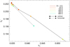 |
Fig. B.1 Comparison of the LDCs of models assuming a vertical (solid line, filled dots) and horizontal (dash-dotted line, filled squares) field configuration. The input field strength is coded by color. |
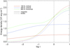 |
Fig. B.2 Comparison of the magnetic (solid lines) and kinetic (dash-dotted lines) energy densities for three different models averaged over surfaces of equal optical Rosseland depth. |
The rather limited spatial resolution of our models implies a significant numerical magnetic (as well momentum) diffusivity. Using an innovative technique, Riva & Steiner (2022) determined the magnetic diffusivity as a function of grid resolution for the C05BOLD code. They found a grid spacing of 12 km as a threshold to allow for small-scale dynamo action in the solar surface layers. This means that in our models small-scale dynamo action cannot be active. However, for us it is of lesser relevance since a certain magnetic flux is enforced by the boundary conditions. The associated field strengths are mostly much larger than the fields expected to emerge from local dynamo action. Eventually, the field strength that we used to label our models should be considered as a parameter measuring the degree of influence of the magnetic fields on the flow structure. Their overall structure, in particular their fine structure, cannot be considered to be fully realistic.
Appendix C Approximate light curve generation and fitting
For the like-for-like comparison it is necessary to be able to synthesize light curves for a given LD law and subsequently analyze these light curves, mimicking an observational procedure. In the general case, the precise calculation of a light curve is fairly involved (see, e.g., Maxted 2016; Morello et al. 2020). Right from the beginning we simplified the necessary calculations by assuming circular orbits for all systems, as indicated by the observations. Moreover, we assumed that: i) the transit chord is a straight path that is equidistantly sampled; ii) the intensity distribution of the host star perpendicular to the transit chord is sufficiently linear that the intensity on the path can be regarded as representative; and iii) the star and the planet are spherical. Figure C.1 illustrates our assumed transit geometry.
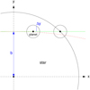 |
Fig. C.1 Illustration of the transit geometry and the chosen coordinate system. The small circles depict the planet at two different locations. The planet has radius R● = 1/10 R⋆ and is transiting the stellar disk (large circle segment) at impact parameter b = 0.7 R⋆. The green line shows the assumed straight transit chord (parallel to the x-axis) and the dashed red line the exact transit chord for a (unrealistically) close-in planet orbiting the host star at a distance of 2 R⋆. ∆y is the extension of the planet perpendicular to the transit chord. For further details, see the text. |
How much stellar flux is blocked by the planetary disk? We assume that the planet is perfectly spherical, with radius R●. Its shape can be expressed as a semicircle with an extension, ∆y● orthogonal to the transit chord, according to
 (C.1)
(C.1)
With this we obtain for the flux that is blocked:
 (C.2)
(C.2)
where I is the intensity toward the observer in the considered passband and b the impact parameter. The factor of two comes about by the fact that the planet extends to “below” as well as “above” the transit cord. As already advertised, Eq. (C.2) is a convolution between the intensity along the transit cord and the shape function of the planetary disk. This can be evaluated efficiently and allows us to work with the sometimes hundreds of light curve calculations necessary for a particular feature in an interactive fashion, which is very convenient. Moreover, it nicely illustrates the “smearing” effect that the planetary disk has on the (indirectly) recorded intensity profile of the star.
Figure C.2 shows a typical example of a resulting light curve and fitted LD curve. M18 fitted the observed transit light curves with a power-2 law. We replicated his approach by fitting power-2 LD curves to the underlying Claret-4 law considered a synthetic “observation”. We sampled the transit path with 2001 points in the range −2 ≤ xplan/R⋆ ≤ 2, where xplan is the geometrical position of the planetary center. The light curve was considered noiseless and each data point was weighted equally. The last assumption is quite reasonable since observationally the photometric precision is little influenced by the small fraction of stellar light blocked by the transiting planet. As stated earlier (see Eqs. (1) and (2)), we formulated our LD laws in terms of absolute intensities, and analogously the blocked flux as an absolute reduction (see Eq. (C.2)). We did constrain the fitting by demanding that the out-of-transit flux obtained from power-2 and the underlying Claret-4 law were the same. This was motivated by the notion that the observed star has a definite brightness that should be matched irrespective of the applied LD law. We used the flux constraint to eliminate the disk center intensity, I(1), from the power-2 law so that we were left with two free parameters. We performed the fitting in (h1, h2), which we subsequently converted to (h′1, h′2). Uncertainties of the fitted parameters (as, e.g., used in Fig. 12) were obtained from the uncertainties on the underlying Claret-4 law by Gaussian error propagation. The necessary Jacobi matrix was calculated numerically, fully accounting for the light curve fitting procedure.
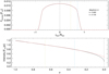 |
Fig. C.2 Typical example of the outcome of the light curve fitting for a non-magnetic model. Upper panel: a comparison between the input light curve based on the Claret-4 law (solid black line), and the fit with a power-2 law (dashed red line). The curves are shown in terms of the light blocked by the planet as a function of its geometrical position, xpian, in units of the stellar radius. Both curves are hardly distinguishable on the scale of the plot. At the given geometry a maximum of μ = 0.8 is reached during transit. Lower panel: input (solid black line) and fitted (dashed red line) LD laws. In both panels, the dashed blue and yellow lines mark locations corresponding to μ = 1/3 and 2/3. For further details, see the text. |
The power-2 law cannot fully match the Claret-4-based LD curves and, as illustrated in the lower panel of Fig. C.2, the biggest differences are generally found in the vicinity of the stellar limb. However, as seen in the upper panel of the figure, this does not have a prominent effect on the light curve as such. Moreover, the parameters used here, (h′1, h′2), are defined using intensities at µ-values where the fitted power-2 law matches the underlying LD curve quite well (see the dashed blue and yellow lines in Fig. C.2). All in all this parallels the observational evidence that the power-2 law is indeed capable of representing the LD of a star reasonably well.
Appendix C.1 Validation of the light curve generation and fitting
It is not obvious what the various simplifications we introduced in our light curve generation and fitting procedure mean in terms of the precision to which we can calculate the LDCs of interest. Based on STAGGER 3D models of Chiavassa et al. (2018), M18 published intensities at various limb angles as well as LDCs derived from these in a like-for-like fashion. We took recourse to these intensity data of M18 and compared the resulting LDCs from our light curve generation and fitting procedure. The data of M18 comprised 80 models covering Teff = 4250… 7000 K, log ɡ ∈ {3.5, 4.0, 4.5, 5.0}, and [Fe/H] ∈ {−0.5, 0.0, +0.5}. For each model, 11 intensities as a function of µ were provided, including µ = 0. M18 interpolate between these values when constructing light curves. In our fitting of Claret laws we had to leave out the point µ = 0 to obtain reasonable fits. Figures C.3 and C.4 show a comparison between our LDCs and the LDCs of M18. The correspondence is excellent without systematic trends, and the remaining differences are immaterial in the context of this investigation. The only limitation in the comparison is that it is restricted to central transits with b = 0. We finally emphasize that the synthetic intensity data of M18 are only used for the validation procedure described here. Otherwise our analysis is exclusively based on our CO5BOLD 3D model data.
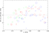 |
Fig. C.3 Differences between the h′1 values calculated in M18 and in this work. The like-for-like calculations were performed for transit parameters b = 0 and k = 0.1. Metallicity is indicated by color: [Fe/H] = +0.5 green, 0.0 red, and -0.5 blue. Larger symbol size indicates lower surface gravity. The expanded ordinate scale should be noted. |
Appendix C.2 Comparison of STAGGER- and C05BOLD-based LDCs
While not immediately pertinent to our investigation, we found a difference between the LDCs presented by M18 and ours that we want to point out here. Figure C.5 depicts LDCs (h′1,h′2) derived from (h1,h2) as published by M18 for the set of models described in the previous section. The LD data of M18 in the h′1,h′2-plane form an almost one-dimensional sequence, with little sensitivity to surface gravity and metallicity. As depicted in Fig. 12, C05BOLD-based LDCs show a clear dependence on log ɡ and [Fe/H] in the range 0.82 ≲ h′1 ≲ 0.86. The reason behind this difference is unclear. However, for the present discussion the apparent difference is perhaps of lesser importance since the main parameter that influences the LDCs is the effective temperature. The sensitivity on Teff is represented quite similarly by C05BOLD and STAGGER.
 |
Fig. C.5 LD coefficients (h′1,h′2) calculated from (h1,h2) published by M18 for the Kepler passband. 80 models are displayed with metallici-ties [Fe/H] = +0.5 in green, 0.0 red, and −0.5 blue. Larger symbol size indicates lower surface gravity. The value of h′1 is predominantly controlled by Teff. |
Appendix D Additive superposition of radiating surface elements following Claret-4 laws
We envision the stellar surface composed of two different kinds of elements, for instance stellar spots and spot-free regions. Each kind of element should exhibit a LD behavior as described by a Claret-4 law. The sizes of the surface elements should be small enough that a transiting hot Jupiter simultaneously covers a sufficient number of elements that all the time a weighted average emission is blocked by the planetary disk. The surface area fractions of the elements we call wa and wb, subject to the normalization condition wa + wb = 1. In the following we show that the additive superposition of emission of the surface elements again follows a Claret-4 law.
The Claret-4 law of Eq. (1) can be alternatively written as
 (D.1)
(D.1)
with LDCs ai and only µ-dependent functions  . Integration of the LD law over a solid angle gives for the emitted flux, F, the relation
 (D.2)
(D.2)
The weighted sum of two surface types, a and b, can be written as
 (D.3)
(D.3)
having the form of a Claret-4 law. Equation (D.2) shows that the resulting flux of a Claret-4 law scales linearly with coefficient zero. This means that by scaling waa0 + wbb0 one can adjust the flux of the additive superposition to any desired value, keeping the functional dependence according a Claret-4 law.
Appendix E Correlation trouble: fitting data subject to strongly correlated uncertainties with non-fitting functions
The statistical uncertainties of the intensity points in the vicinity of the disk center are highly correlated. Initially, we had the intention to fully include these correlations in the fitting of the LD laws. However, this resulted in unreasonable-looking fits. In fact, the fits did not pass close to any of the provided data points at all. For that reason we decided to leave out the correlations when performing the fitting. In the following, we discuss a simple, analytically tractable example that illustrates the issue (see, e.g., Hogg et al. 2010, for a general discussion on maximum likelihood fitting). The central problem turns out to be related to the fact that the fitting function does not correspond to the true generative function that underlies the data. It should be appreciated that in astronomy this situation is the rule rather than the exception, that is to say, it is frequently encountered in practice.
We consider two points, A and B, located at positions
 (E.1)
(E.1)
in a two-dimensional (x, y)-plane. The x-coordinates of the points are exactly known; the y-coordinates have uncertainties of the same magnitude, σ, which follow a Gaussian distribution. A straight line of the form
 (E.2)
(E.2)
is going to be fitted through the points where λ is the fitting parameter. The function (E.2) has a fix-point at (−1, 0) (see Fig. E.1), and hence cannot pass through point A at (−1, 1) for any choice of λ ∈] – ∞, ∞[. The function is in this sense defective – as desired for the purpose of this illustration.
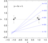 |
Fig. E.1 Illustration of a fitting problem when correlations among the uncertainties of the data are present. For details, see the text. |
We want to discuss the effect of correlated uncertainties. In the presence of mutual correlations among the uncertainties at points A and B, the covariance matrix C can be written as
 (E.3)
(E.3)
with the linear correlation coefficient r ∈ [−1, 1]. The inverse of the covariance matrix, C−1, is given by
 (E.4)
(E.4)
so that the,χ2(λ) of the fitting problem is
![Mathematical equation: $ {\chi ^2} = {\rm{\Delta }}{{\bf{y}}^{\rm{T}}}{C^{ - 1}}{\rm{\Delta }}{\bf{y}} = {{2\left[ {1 - r - 2\lambda \left( {1 - r - \lambda } \right)} \right]} \over {{\sigma ^2}\left( {1 - {r^2}} \right)}}, $](/articles/aa/full_html/2023/11/aa46783-23/aa46783-23-eq47.png) (E.5)
(E.5)
where
 (E.6)
(E.6)
is the vector of ordinate differences, and (.)T denotes the transpose. Figure E.2 depicts the χ2-function according to Eq. (E.5) in the space of ordinate differences. The surface area, A, enclosed by the contour χ2 = 1 is
 (E.7)
(E.7)
showing the reduction in the size of the confidence region with the increasing degree of correlations (independent of sign), accompanied by a reduction in the uncertainty of the best fitting λ, as shown in the following.
Minimizing χ2 with respect to λ provides an estimate,
 (E.8)
(E.8)
with a variance,
 (E.9)
(E.9)
and minimum χ2 (λest) of
 (E.10)
The result for λest (see again Fig. E.1) in the case r = 0 is plausible: the distance between the fitted line and point В is made zero. This is obviously the best that can be achieved, given that there is no way to reduce the (vertical) distance between the fitted curve and point A. It is quite striking to see that for r ≠ 0 the fitted line never passes through any of the given points. For the strong positive correlation r→ lit runs parallel to the given points at some distance. Qualitatively, this is what we observe when trying to fit our intensity data with the Claret-4 law, including the strong positive correlation among the uncertainties of the data points.
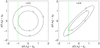 |
Fig. E.2 Maps of χ2 according Eq. (E.5). Two examples for a different degree of correlation, r, are shown. In both cases σ2 = 1 is assumed. Contour lines illustrate the situation for arbitrary deviations from (yA, yB), the green line the one-dimensional subset selected by the fitting function (E.2). The green dot marks the best fitting λ. Short streaks indicate the uncertainty. |
On a side note, Eq. (E.9) shows that the inclusion of correlations (r ≠ 0) at a fixed variance of the data leads to a higher precision of the fitted parameter, λ. Moreover, according to Eq. (E.10) the minimumχ2 turns out to be the same irrespective of the degree of correlation – at least in this particular example. This tells one that fits that do not pass through data points due to the inclusion of correlations have by no means generally a greater χ2 than a fit that manages to pass at least through some data points by ignoring correlations, which is also graphically shown in Fig. E.2.
Appendix F Comments on Maxted’s observational results of 2023
In 2023 Maxted (see M23) extended the observational basis to 34 transiting systems with high-quality light curves obtained by Kepler which we plotted in Fig. F.1. Unlike his work reported in M18, he fitted the observed light curves assuming a Claret-4 law for the LD. We did not follow his approach here, and performed the like-for-like calculation of the LDCs still assuming a power-2 law. We do not consider this inconsistency to be vital since – as shown before – the effects are small at low field strengths. The larger number of free parameters in the Claret-4 law led to an unfortunately large increase in the uncertainty of the observationally derived LDCs. For that reason we decided to remove the observed systems from further analysis with an overly large uncertainty (area of confidence region > 5 × 10⁻⁴). Only 12 systems remained after cleansing, of which only four were new, and hence there was little information gain in comparison to the sample of M18. Moreover, the resulting overall picture is less clear since two objects lie outside the region that is plausibly accessible by MHD models.
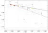 |
Fig. F.1 Like Fig. 14 but showing a subset of observational results of M23 selected for their small uncertainties. |
Appendix G Fits of the MHD models with Claret-6 laws
Figures G.1 and G.2 illustrate that the Claret-6 law provides a very good representation of the temporally and horizontally averaged intensity distribution of our MHD models. Since it is potentially useful for comparison purposes, we provide the fitting coefficients of the Claret-6 laws in Tab. G.l. We caution that most coefficients are highly correlated so that formal uncertainties are large and individual coefficients are not well defined. Alternative parameter combinations can provide almost equally good representations.
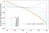 |
Fig. G.1 Fits to the MHD intensity distributions with the Claret-6 law. The unit of intensity differs among models. |
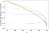 |
Fig. G.2 Fits to the MHD intensity distributions with the Claret-6 law. The same unit of intensity is used for all models emphasizing the reduction in total flux at great magnetic field strengths. The color-model correspondence is the same as in Fig. G.1. |
Appendix H Intensity data and intensity ratios close to the stellar limb
The tables in this section list the intensity data used in this investigation. Tables H.1 to H.3 provide the intensities for various limb angles, as well as the intensity ratios applied to regularize fits. All values have been corrected for sphericity effects in the radiative transfer (but not the model structure as such). In any case, except for limb angles μ ≲ 0.05, the corrections are small and do not change our results significantly. Absolute intensities are given in terms of photon counts since the detectors of Kepler are essentially photon counting devices. We started this investigation having only intensities at Lobatto angles available. Later on, we supplemented the MHD models with angles according to a Gauss-Radau scheme. The rationale was simply that both sets are roughly interleaved so that one obtains a finer stepping in μ. Moreover, the Gauss-Radau angles extend further to the limb. This is reflected in a separation into two tables (besides formatting reasons). As explained in the main text, we also list the intensity ratios that we introduced to regularize fits close to the stellar limb.
Besides the intensities proper, the tables also list the statistical uncertainties (1σ) that we applied when fitting the intensities with LD laws. We note that the uncertainties are heavily correlated; however, due to the problem laid out in Appendix E, we chose to neglect the correlations. We increased the uncertainty of the intensity ratio by a factor of ten in an ad-hoc fashion. Our motivation was that we considered these ratios to only be approximate since they were obtained using a gray approximation.
Tables H.4 to H.6 correspond precisely to the previous tables except that a (rather high) interstellar extinction of AV = 1 mag was applied. We used the extinction law provided by Cardelli et al. (1989, their equations 1 and 2).
References
- Beeck, B., Schüssler, M., Cameron, R. H., & Reiners, A. 2015, A&A, 581, A42 [NASA ADS] [CrossRef] [EDP Sciences] [Google Scholar]
- Bhatia, T. S., Cameron, R. H., Solanki, S. K., et al. 2022, A&A, 663, A166 [NASA ADS] [CrossRef] [EDP Sciences] [Google Scholar]
- Bonifacio, P., Caffau, E., Ludwig, H. G., et al. 2018, A&A, 611, A68 [NASA ADS] [CrossRef] [EDP Sciences] [Google Scholar]
- Borucki, W. J., Koch, D., Basri, G., et al. 2010, Science, 327, 977 [Google Scholar]
- Cardelli, J. A., Clayton, G. C., & Mathis, J. S. 1989, ApJ, 345, 245 [Google Scholar]
- Carlsson, M., Stein, R. F., Nordlund, Å., & Scharmer, G. B. 2004, ApJ, 610, L137 [NASA ADS] [CrossRef] [Google Scholar]
- Castelli, F., & Kurucz, R. L. 2003, in Modelling of Stellar Atmospheres, 210, eds. N. Piskunov, W. W. Weiss, & D. F. Gray, A20 [NASA ADS] [Google Scholar]
- Chen, F., Rempel, M., & Fan, Y. 2017, ApJ, 846, 149 [Google Scholar]
- Chiavassa, A., Casagrande, L., Collet, R., et al. 2018, A&A, 611, A11 [NASA ADS] [CrossRef] [EDP Sciences] [Google Scholar]
- Claret, A. 2000, A&A, 363, 1081 [NASA ADS] [Google Scholar]
- Csizmadia, S., Pasternacki, T., Dreyer, C., et al. 2013, A&A, 549, A9 [NASA ADS] [CrossRef] [EDP Sciences] [Google Scholar]
- Espinoza, N., & Jordán, A. 2016, MNRAS, 457, 3573 [NASA ADS] [CrossRef] [Google Scholar]
- Freytag, B., Steffen, M., Ludwig, H.-G., et al. 2012, J. Comput. Phys., 231, 919 [Google Scholar]
- Gallagher, A. J., Steffen, M., Caffau, E., et al. 2017, Mem. Soc. Astron. Italiana, 88, 82 [NASA ADS] [Google Scholar]
- Hestroffer, D. 1997, A&A, 327, 199 [NASA ADS] [Google Scholar]
- Hogg, D. W., Bovy, J., & Lang, D. 2010, ArXiv e-prints, [arXiv:1008.4686] [Google Scholar]
- Howarth, I. D. 2011, MNRAS, 413, 1515 [NASA ADS] [CrossRef] [Google Scholar]
- Ji, Y. 2021, Master’s thesis, Heidelberg University, Germany [Google Scholar]
- Kervella, P., Bigot, L., Gallenne, A., & Thévenin, F. 2017, A&A, 597, A137 [NASA ADS] [CrossRef] [EDP Sciences] [Google Scholar]
- Kostogryz, N. M., Witzke, V., Shapiro, A. I., et al. 2022, A&A, 666, A60 [NASA ADS] [CrossRef] [EDP Sciences] [Google Scholar]
- Kucinskas, A., Klevas, J., Ludwig, H. G., et al. 2018, A&A, 613, A24 [NASA ADS] [CrossRef] [EDP Sciences] [Google Scholar]
- Lanza, A. F., Netto, Y., Bonomo, A. S., et al. 2019, A&A, 626, A38 [NASA ADS] [CrossRef] [EDP Sciences] [Google Scholar]
- Ludwig, H.-G., & Kucinskas, A. 2012, A&A, 547, A118 [NASA ADS] [CrossRef] [EDP Sciences] [Google Scholar]
- Ludwig, H. G., Jordan, S., & Steffen, M. 1994, A&A, 284, 105 [NASA ADS] [Google Scholar]
- Ludwig, H.-G., Caffau, E., Steffen, M., et al. 2009, Mem. Soc. Astron. Italiana, 80, 711 [NASA ADS] [Google Scholar]
- Magic, Z., Collet, R., Asplund, M., et al. 2013, A&A, 557, A26 [NASA ADS] [CrossRef] [EDP Sciences] [Google Scholar]
- Markwardt, C. B. 2009, ASP Conf. Ser., 411, 251 [Google Scholar]
- Maxted, P. F. L. 2016, A&A, 591, A111 [NASA ADS] [CrossRef] [EDP Sciences] [Google Scholar]
- Maxted, P. F. L. 2018, A&A, 616, A39 [NASA ADS] [CrossRef] [EDP Sciences] [Google Scholar]
- Maxted, P. F. L. 2023, MNRAS, 519, 3723 [NASA ADS] [CrossRef] [Google Scholar]
- Moré, J. J. 1978, in Lecture Notes in Mathematics, 630 (Berlin: Springer Verlag), 105 [CrossRef] [Google Scholar]
- Morello, G., Claret, A., Martin-Lagarde, M., et al. 2020, AJ, 159, 75 [NASA ADS] [CrossRef] [Google Scholar]
- Morello, G., Gerber, J., Plez, B., et al. 2022, RNAAS, 6, 248 [NASA ADS] [Google Scholar]
- Neilson, H. R., & Lester, J. B. 2013, A&A, 556, A86 [CrossRef] [EDP Sciences] [Google Scholar]
- Nordlund, A. 1982, A&A, 107, 1 [Google Scholar]
- Norris, C. M., Beeck, B., Unruh, Y. C., et al. 2017, A&A, 605, A45 [NASA ADS] [CrossRef] [EDP Sciences] [Google Scholar]
- Panja, M., Cameron, R., & Solanki, S. K. 2020, ApJ, 893, 113 [CrossRef] [Google Scholar]
- Panja, M., Cameron, R. H., & Solanki, S. K. 2021, ApJ, 907, 102 [Google Scholar]
- Patel, J. A., & Espinoza, N. 2022, AJ, 163, 228 [NASA ADS] [CrossRef] [Google Scholar]
- Rempel, M., Schüssler, M., & Knölker, M. 2009, ApJ, 691, 640 [Google Scholar]
- Riva, F., & Steiner, O. 2022, A&A, 660, A115 [NASA ADS] [CrossRef] [EDP Sciences] [Google Scholar]
- Riva, F., Steiner, O., & Freytag, B. 2023, A&A, submitted [Google Scholar]
- Salhab, R. G., Steiner, O., Berdyugina, S. V., et al. 2018, A&A, 614, A78 [NASA ADS] [CrossRef] [EDP Sciences] [Google Scholar]
- Schüssler, M., & Vögler, A. 2006, ApJ, 641, L73 [Google Scholar]
- Sing, D. K., Vidal-Madjar, A., Désert, J. M., Lecavelier des Etangs, A., & Ballester, G. 2008, ApJ, 686, 658 [Google Scholar]
- Steffen, M., Ludwig, H.-G., Wedemeyer, S., & Gallagher, A. J. 2022, Linfor3D User Manual [Google Scholar]
- Stein, R. F., & Nordlund, Å. 2006, ApJ, 642, 1246 [NASA ADS] [CrossRef] [Google Scholar]
- Steiner, O., Salhab, R., Freytag, B., et al. 2014, PASJ, 66, S5 [NASA ADS] [Google Scholar]
- Trampedach, R., Asplund, M., Collet, R., Nordlund, Å., & Stein, R. F. 2013, ApJ, 769, 18 [NASA ADS] [CrossRef] [Google Scholar]
- Tremblay, P.-E., Ludwig, H.-G., Freytag, B., Steffen, M., & Caffau, E. 2013, A&A, 557, A7 [NASA ADS] [CrossRef] [EDP Sciences] [Google Scholar]
- Unsöld, A. 1968, Physik der Sternatmosphären mit besonderer Berücksichtigung der Sonne (Springer Verlag) [Google Scholar]
- Valio, A., Estrela, R., Netto, Y., Bravo, J. P., & de Medeiros, J. R. 2017, ApJ, 835, 294 [CrossRef] [Google Scholar]
- Van Cleve, J., Caldwell, D., Thompson, R., et al. 2009, Kepler Instrument Handbook, https://keplergo.github.io/KeplerScienceWebsite/data/documentation/KSCI-19033-001.pdf [Google Scholar]
- Vitas, N. 2011, PhD thesis, University of Utrecht, The Netherlands [Google Scholar]
- Vögler, A. 2005, Mem. Soc. Astron. Italiana, 76, 842 [Google Scholar]
- Vögler, A., & Schüssler, M. 2007, A&A, 465, L43 [Google Scholar]
- Witzke, V., Duehnen, H. B., Shapiro, A. I., et al. 2023, A&A, 669, A157 [NASA ADS] [CrossRef] [EDP Sciences] [Google Scholar]
Minor and major axes of the error ellipses are shown; they appear not orthogonal in the plot since the scaling of abscissa and ordinate differs.
All Tables
Direction cosines of the two different ray configurations discussed in this paper.
Approximate ranking of the systems analyzed by M18 in order of increasing field strength.
All Figures
|
Fig. 1 Processing steps of the CLV analysis. References to the most relevant sections of the steps are given in angular brackets. |
| In the text | |
|
Fig. 2 Mean T(τ)-relations of the nine MHD simulations. |
| In the text | |
|
Fig. 3 Temperature fluctuations on surfaces of equal optical depth of the nine MHD simulations. |
| In the text | |
|
Fig. 4 Bolometric emergent intensity viewed at different limb angles for four MHD models with В = 0, 800,1600, 2400 G. For each model a selected snapshot is shown, ordered upper-left to lower-right. The gray scale is kept the same for each viewing angle of a particular snapshot. The increasing impact of the magnetic fields is apparent by the transition from quiet photosphere to sun-spot (umbral) conditions. |
| In the text | |
|
Fig. 5 32 HD models (red and blue dots) together with observational data (gray symbols) from M23 in the Teff-log ɡ-plane. Red indicates models of solar; blue models of 1/10 solar metallicity. The subset of systems also analyzed in M18 is depicted by gray squares. Most of the observed systems have slightly super-solar metallicity. One system with Teff < 4000 K is not shown. |
| In the text | |
|
Fig. 6 Example (field-free model B0000) of the calculated intensity distribution, together with the Kepler passband. The reddening effect on the passband from interstellar extinction of 1 mag is depicted. Passbands are normalized to a maximum of one. Since Kepler effectively operates in photon-counting mode, intensities are expressed in terms of photon counts. |
| In the text | |
|
Fig. 7 Illustration of the ray geometry in spherical (upper half) and plane-parallel (lower half) symmetry. Gray regions correspond to the optically thick regions of the star. R⋆ is the stellar radius, z the vertical coordinate, and rtop the – somewhat arbitrary – uppermost level in the spherical or planar atmosphere. Red arrows depict how straight light rays in spherical geometry get bent when interpreted in planar geometry. The blue arrow depicts a ray in planar geometry. The yellow circle marks the location where the inclination angle of rays in both geometries coincides. The green angle illustrates the inclination angle of a ray with respect to the vertical. “Core rays” are rays that penetrate into the optically thick part of a star. |
| In the text | |
|
Fig. 8 Intensity proflies at the extreme stellar limb of the nine MHD models. The solid lines are the fitted intensity profiles using the Claret-4 law. The dashed lines depict the result of radiative transfer calculations along tangential rays in the gray approximation. The dots to the right mark the position μ = 0 (the location of the stellar radius), and the dots to the left μ = 0.04. The solid lines end at dots marking μ = 0 as the stellar limb and limit of definition of the Claret–4 law. For clarity, the curves were scaled in steps of factors of two in the vertical direction, with model В = 0 G at its original position. In this plot, the zero points of the z-scales are located at a radial Rosseland optical depth of one in the respective model. |
| In the text | |
|
Fig. 9 Comparison of intensities in the Kepler passband calculated in spherical and plane-parallel symmetry. The results are shown for two models of approximately solar effective temperature and metallicity but different surface gravity. For clarity, the intensities of the log ɡ = 3.5 model were scaled by a factor of two. The intensities were calculated in the gray approximation. |
| In the text | |
|
Fig. 10 Time-resolved synthetic intensities of the nine MHD models (open circles) fitted with the Claret-6 law (solid lines; color encodes the model) to guide the eye. Intensities are given in units of the temporal average of the mean surface brightness of each model; that is, the unit of intensity is temporally fixed for each model but differs among them. No corrections for sphericity effects were applied. |
| In the text | |
|
Fig. 11 Time-averaged synthetic intensities of the nine MHD models fitted with a Claret-4 law. Filled circles and solid lines depict the result for the Lobatto angles; open circles and dash-dotted lines the result when Gauss-Radau angles are added. Intensities are given in units of the mean surface brightness of each model. Corrections for sphericity effects were applied. For further details, see the text. |
| In the text | |
|
Fig. 12 Example of polynomial fits in stellar parameter space to h′1 and h′2 from light curve analyses for transit parameters b = 0 and k = 0.1. Red dots with 1σ joint confidence regions depict the results of 3D models of solar metallicity, and blue dots the results for metallicity [Fe/H] = −1. Lines of constant Teff and log ɡ are added to illustrate the functional dependence. Line segments connect data points and corresponding values predicted by the polynomial. |
| In the text | |
|
Fig. 13 Comparison between observations of M18 and calculations in the h′1-h′2-plane. Symbols in color depict the results from solar MHD simulations. Gray and black symbols show the observational data. Data points before and after normalization are connected by a line. The solid black line labeled with field strengths is a fit to the MHD models to guide the eye. The dash-dotted line illustrates the outcome of an additive mixing of models B0050 and B1600, where percentages give the area fraction contributed by B1600. See the text for more explanations on the approach. The colored arrows indicate the sensitivity of the (h′1, h′2)-vector to the atmospheric parameters. |
| In the text | |
|
Fig. 14 Like Fig. 13 but zoomed in on the region with the observational data. The ellipses show their 1σ joint confidence regions. The best-guess solar position as obtained from model B0000 after normalization is marked by the solar symbol. |
| In the text | |
|
Fig. 15 Effect of extinction: filled circles depict the standard LDCs (h′1, h′2) without interstellar extinction; filled stars depict them when assuming an extinction of AV = 1 mag. All data are normalized to solar conditions. The solid black line with labels is a fit to the reddening-free data points; the dashed violet line to the reddened ones. The coloring of the symbols according to field strength follows our standard color scheme. |
| In the text | |
|
Fig. A.1 Comparison of emergent intensities in the Kepler passband calculated using wavelength-independent Rosseland opacities (“gray”), and wavelength-dependent opacities based on opacity distribution functions (“ODF”). The results for the four mean structures of MHD models are depicted assuming plane-parallel symmetry. |
| In the text | |
|
Fig. B.1 Comparison of the LDCs of models assuming a vertical (solid line, filled dots) and horizontal (dash-dotted line, filled squares) field configuration. The input field strength is coded by color. |
| In the text | |
|
Fig. B.2 Comparison of the magnetic (solid lines) and kinetic (dash-dotted lines) energy densities for three different models averaged over surfaces of equal optical Rosseland depth. |
| In the text | |
|
Fig. C.1 Illustration of the transit geometry and the chosen coordinate system. The small circles depict the planet at two different locations. The planet has radius R● = 1/10 R⋆ and is transiting the stellar disk (large circle segment) at impact parameter b = 0.7 R⋆. The green line shows the assumed straight transit chord (parallel to the x-axis) and the dashed red line the exact transit chord for a (unrealistically) close-in planet orbiting the host star at a distance of 2 R⋆. ∆y is the extension of the planet perpendicular to the transit chord. For further details, see the text. |
| In the text | |
|
Fig. C.2 Typical example of the outcome of the light curve fitting for a non-magnetic model. Upper panel: a comparison between the input light curve based on the Claret-4 law (solid black line), and the fit with a power-2 law (dashed red line). The curves are shown in terms of the light blocked by the planet as a function of its geometrical position, xpian, in units of the stellar radius. Both curves are hardly distinguishable on the scale of the plot. At the given geometry a maximum of μ = 0.8 is reached during transit. Lower panel: input (solid black line) and fitted (dashed red line) LD laws. In both panels, the dashed blue and yellow lines mark locations corresponding to μ = 1/3 and 2/3. For further details, see the text. |
| In the text | |
|
Fig. C.3 Differences between the h′1 values calculated in M18 and in this work. The like-for-like calculations were performed for transit parameters b = 0 and k = 0.1. Metallicity is indicated by color: [Fe/H] = +0.5 green, 0.0 red, and -0.5 blue. Larger symbol size indicates lower surface gravity. The expanded ordinate scale should be noted. |
| In the text | |
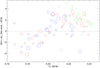 |
Fig. C.4 Like Fig. C.3 but for parameter h′2. |
| In the text | |
|
Fig. C.5 LD coefficients (h′1,h′2) calculated from (h1,h2) published by M18 for the Kepler passband. 80 models are displayed with metallici-ties [Fe/H] = +0.5 in green, 0.0 red, and −0.5 blue. Larger symbol size indicates lower surface gravity. The value of h′1 is predominantly controlled by Teff. |
| In the text | |
|
Fig. E.1 Illustration of a fitting problem when correlations among the uncertainties of the data are present. For details, see the text. |
| In the text | |
|
Fig. E.2 Maps of χ2 according Eq. (E.5). Two examples for a different degree of correlation, r, are shown. In both cases σ2 = 1 is assumed. Contour lines illustrate the situation for arbitrary deviations from (yA, yB), the green line the one-dimensional subset selected by the fitting function (E.2). The green dot marks the best fitting λ. Short streaks indicate the uncertainty. |
| In the text | |
|
Fig. F.1 Like Fig. 14 but showing a subset of observational results of M23 selected for their small uncertainties. |
| In the text | |
|
Fig. G.1 Fits to the MHD intensity distributions with the Claret-6 law. The unit of intensity differs among models. |
| In the text | |
|
Fig. G.2 Fits to the MHD intensity distributions with the Claret-6 law. The same unit of intensity is used for all models emphasizing the reduction in total flux at great magnetic field strengths. The color-model correspondence is the same as in Fig. G.1. |
| In the text | |
Current usage metrics show cumulative count of Article Views (full-text article views including HTML views, PDF and ePub downloads, according to the available data) and Abstracts Views on Vision4Press platform.
Data correspond to usage on the plateform after 2015. The current usage metrics is available 48-96 hours after online publication and is updated daily on week days.
Initial download of the metrics may take a while.