| Issue |
A&A
Volume 679, November 2023
|
|
|---|---|---|
| Article Number | A118 | |
| Number of page(s) | 10 | |
| Section | Astrophysical processes | |
| DOI | https://doi.org/10.1051/0004-6361/202346483 | |
| Published online | 29 November 2023 | |
Probing cosmic ray escape from η Carinae
Max-Planck-Institut für Kernphysik, Postfach 103980, 69029 Heidelberg, Germany
e-mail: This email address is being protected from spambots. You need JavaScript enabled to view it.
; This email address is being protected from spambots. You need JavaScript enabled to view it.
Received:
22
March
2023
Accepted:
6
September
2023
Abstract
The binary stellar system η Carinae is one of very few established astrophysical hadron accelerators. It seems likely that at least some fraction of the particles accelerated by η Carinae escape from the system. Copious target material for hadronic interactions and associated γ-ray emission exist on a wide range of spatial scales outside the binary system. This material creates a unique opportunity to trace the propagation of particles into the interstellar medium. In this work, we analyse γ-ray data from Fermi-LAT of η Carinae and surrounding molecular clouds and investigate the many different scales on which escaping particles may interact and produce γ-rays. We find that interactions of escaping cosmic rays from η Carinae in the wind region and the Homunculus Nebula could produce a significant contribution to the γ-ray emission associated with the system. Furthermore, we detect excess emission from the surrounding molecular clouds. The derived radial cosmic-ray excess profile is consistent with a steady injection of cosmic rays by a central source. However, this would require a higher flux of escaping cosmic rays from η Carinae than provided by our model. Therefore, it is likely that additional cosmic ray sources contribute to the hadronic γ-ray emission from the clouds.
Key words: radiation mechanisms: non-thermal / gamma rays: stars / stars: winds / outflows / stars: individual: η Carinae / cosmic rays
© The Authors 2023
 Open Access article, published by EDP Sciences, under the terms of the Creative Commons Attribution License (https://creativecommons.org/licenses/by/4.0), which permits unrestricted use, distribution, and reproduction in any medium, provided the original work is properly cited.
This article is published in open access under the Subscribe to Open model.
Open access funding provided by Max Planck Society.
1. Introduction
Colliding wind binaries (CWBs) are a well-established class of Galactic particle accelerator, with non-thermal emission seen from a number of systems (Moran et al. 1989; Churchwell et al. 1992; Contreras & Rodríguez 1999; Dougherty & Williams 2000; Marcote et al. 2021; del Palacio et al. 2023). In γ-rays, only two systems have been detected so far: η Carinae (e.g., Abdo et al. 2010a) and γ2 Velorum (Martí-Devesa et al. 2020), located (2.35 ± 0.05) kpc (Smith 2006) and (0.34 ± 0.01) kpc (North et al. 2007) from Earth, respectively. Of the two systems, η Carinae (henceforth η Car) is the more luminous, and it has therefore been studied in greater detail. Over its 15-year lifetime, the Fermi Large Area Telescope (LAT) has probed three periastron passages of this highly eccentric (ϵ ≈ 0.9, Mehner et al. 2015) CWB with an orbital period of ∼5.5 yr (e.g., Damineli et al. 2008; Teodoro et al. 2016). The high eccentricity and relatively short orbital period, combined with its dense matter and photon fields, make η Carinae a unique source in which to study high-energy astrophysical processes in a time-dependent environment.
The Astro-Rivelatore Gamma a Immagini Leggero (AGILE) satellite was used to detect η Car for the first time in γ-rays (Tavani et al. 2009). The detection was soon confirmed by observations with the Fermi-LAT satellite (Abdo et al. 2010a; Nolan et al. 2012). Since then, several works have analysed the γ-ray emission measured by Fermi-LAT (Abdo et al. 2010b; Farnier et al. 2011; Reitberger et al. 2012, 2015; Balbo & Walter 2017; White et al. 2020; Martí-Devesa & Reimer 2021; Abdollahi et al. 2022a). Two components are apparent in the emitted spectrum above and below ∼10 GeV (see e.g., Abdo et al. 2010b; Farnier et al. 2011). During the periastron phase, which is when the stars are closest to each other, the emission increases. The peak emission at GeV energies around periastron increases by ∼40% relative to the baseline flux (Martí-Devesa & Reimer 2021). Emission up to 400 GeV has now been established using the High Energy Stereoscopic System (H.E.S.S.; H.E.S.S. Collaboration 2020).
The γ-ray emission from η Car is generally believed to be emitted by cosmic rays (CRs) accelerated by the shocks that enclose the wind collision region (WCR), where the supersonic winds from the two stars collide to form a pair of standing shocks, separated by a contact discontinuity. The shocks are approximately located at the surface (cap) where the ram pressures from both winds are equal. At the shocks, electrons and protons can be accelerated to relativistic energies and emit γ-rays via synchrotron and inverse Compton processes or via proton-proton collisions with subsequent π0-decay. For the latter process, a dense target material is needed to produce a detectable γ-ray signal. Bednarek & Pabich (2011) were the first to point out that the two shocks in the system should have distinct properties due to the different stellar mass loss rates and terminal wind velocities. These properties result in two different accelerated particle populations. These ideas were developed further in the work by Ohm et al. (2015) and White et al. (2020; henceforth O15 and W20, respectively), where models were constructed to account for the variable γ-ray emission observed by Fermi-LAT and the non-thermal X-ray emission detected with the NuSTAR satellite (Hamaguchi et al. 2018). In W20, a non-negligible amount of the accelerated protons escape the WCR. Such particles would naturally interact with the surrounding material further out.
The complex environment around η Car provides many potential interaction regions. Though the inner structures, including the binary system and its immediate vicinity, cannot be resolved by Fermi-LAT or H.E.S.S., the nearby molecular clouds in the Carina Nebula Complex (CNC) and nearby Gum 31 are resolvable. Significant emission associated with these clouds above the expectations for the ‘sea’ of diffuse CRs was reported in W20. In this work, we explore this emission in more detail.
Recently, Ge et al. (2022) published an analysis of the excess γ-ray emission around η Car considering two Gaussian regions, for which significant emission (likely of hadronic origin) was found. They concluded that the emission could be connected to young massive stellar clusters in the region, such as Trumpler 14 and 16. Nevertheless, the authors were not able to rule out that η Car or yet unknown CR sources are the acceleration sites of the particles producing the γ-ray emission.
In this article, we follow up on these ideas and perform a detailed analysis of the emission from η Car and the surrounding excess emission considering not two but four different regions. These regions correspond to specific nearby molecular cloud structures connected to the Carina Nebula-Gum 31 complex. Additionally, we analyse possible γ-ray emission from escaping CRs interacting with material on small and large scales around η Car.
While this work focuses primarily on escaping particles accelerated in the WCR, it is also possible that particles have been accelerated in the blast wave from the great eruption of 1843, when the system released more than 10 M⊙ of material (Smith 2006) with high velocity (Ohm et al. 2010; Skilton et al. 2012). While the apparent orbital variability effectively rules out the possibility that all emission from η Car is due to the blast wave, a significant fraction of the steady emission could still be produced near the blast wave. Though we do not consider them further in this work, these particles would also contribute to the γ-ray emission on larger scales.
The paper is structured as follows: In Sect. 2, we present an overview of the environment around η Car. This is followed by the analysis of the Fermi-LAT data in Sect. 3. Afterwards, we explore possible γ-ray emission from escaping particles on scales not resolvable by Fermi-LAT (Sect. 4) and in the molecular clouds on larger scales (Sect. 5). Finally, we discuss our findings in Sect. 6.
2. Environment around η Car
The surroundings in which the η Car binary system is embedded are non-homogeneous, with multiple complex structures on a variety of scales. These structures provide not only a variety of target conditions for CRs escaping from η Car but also multiple competing sites for particle acceleration. We considered the following zones, in order of increasing scale, as targets for CR interactions and γ-ray emission:
The first zone we considered was the shock cap, or WCR. It is the region where the shocks form between the two stars. Following W20, we refer to the more massive star as η Car-A and the lower mass companion as η Car-B. This zone is depicted as region A in Fig. 1.
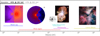 |
Fig. 1. Scales relevant to the possible emission regions around η Car. Because some regions, such as the large and the little Homunculus nebulae, are asymmetric or have sizes that can change over time, such as for the shock cap, the sizes shown cover a large range of values. The different extensions are as follows: 1–20 au (shock cap, A); 10–6.4 × 10³ au (wind region, B); 2 × 10³ to 6.5 × 10³ au (little Homunculus, C); 2.1 × 10³ to 21.69 × 10³ au (Homunculus, D); and > 50 × 103 au (Carina Nebula, E). The black and grey bars in the upper-left corner indicate the distances beyond which the absorption at 200 GeV is less than 50% (black) and the absorption at 600 GeV is less than 10% (grey), see text for more details. The individual images are from Parkin et al. (2011), Clementel et al. (2014), Smith (2005), HST, and ESO. |
The second zone was the pinwheel and wind region, which is a high-velocity outflow with gradual mixing of the high- and low-density winds of the two stars ending on the scale of the little Homunculus (a possible remnant of an outburst more recent than the great eruption). This zone is depicted as region B in Fig. 1.
The third zone was the Homunculus. This is the expanding shell associated with the great eruption of 1843. This zone is depicted as region D in Fig. 1.
The fourth zone we considered was the Carina Nebula-Gum 31 complex, which is the star formation region containing several massive stellar clusters and 103–105 solar mass molecular clouds (see e.g., Rebolledo et al. 2016). This zone is depicted as region E in Fig. 1.
Figure 1 provides detailed illustrations of these different regions. The approximate sizes of these regions are indicated by the coloured lines below each graphic. Additionally, we show the approximate spatial scales associated with the absorption of the γ-rays. To compute these scales, the stellar parameters were taken to be the same as in W20, and the angular size of the stars was taken into account. While the absorption in W20 was calculated specifically for the emitting region and integrated for specific orbital phase ranges, in this paper we adopted a spherical geometry of the γ-ray emission region for simplicity, and the two stars were taken to be at their maximum separation, that is, the apastron position. The black line in the top-left part of the figure shows the radii for which more than 50% of γ-rays with an energy of 200 GeV would be absorbed before reaching Earth. The peak absorption occurs close to 600 GeV, and the adjacent grey line shows the radial distances inside which more than 10% of these 600 Gev γ-rays are absorbed. Therefore, accounting for γ-ray absorption is essential for the emission within ∼200 au of the stars. A detailed plot showing the radial dependence for different energies is provided in Appendix B.
The shock cap, or WCR, is formed by the colliding stellar winds. As discussed previously, the winds terminate in a pair of shocks separated by a contact discontinuity. The shock cap refers to its finite lateral extent. The global size of this region varies, with the orbital phase between ∼1 au at periastron and ∼20 au at apastron. At the shocks, particles are expected to be accelerated (see e.g., Eichler & Usov 1993). A detailed discussion of the particle acceleration and emission can be found in O15 and W20.
The shock cap and associated pinwheel are embedded in the wind region, which is created by the outflowing winds from both stars. Due to the orbital motion, the winds create a pinwheel-like structure; but for η Carinae this structure is complicated by its eccentric orbit (see Parkin & Pittard 2008). From simulations, Madura et al. (2013; see also Parkin et al. 2011; Clementel et al. 2014) found that the fast wind from η Car-B carves out a low-density channel with a large opening angle in the direction of the apastron position. This is a consequence of the brief periastron passage. As is evident in image B in Fig. 1, the darker region indicates the low-density wind from η Car-B. Accelerated particles that enter this region experience negligible collisions. However, any particles that encounter denser wind material from η Car-A within ≈100 au from the binary become collision dominated and have a low probability of escaping the wind region.
The wind region is expected to end as it reaches the little Homunculus Nebula (see Fig. 1C). This nebula has a total mass of plausibly ∼0.1 M⊙ (Smith 2005). It is believed to have been ejected in the outburst from 1890 and accelerated by the stellar winds. It has a bipolar shape, with the equator being ∼2 × 10³ au and its poles around 6.5 × 10³ au away from the central stars.
The little Homunculus itself is embedded in the larger Homunculus Nebula, the large bipolar structure shown in image D of Fig. 1. The Homunculus was ejected during the great eruption of η Car in the 1840s. It is mainly composed of a thin outer shell, with a thickness of up to 600 au, and a thicker inner shell (Smith 2006). The thin outer shell contains ∼90% of the total mass of the Homunculus. The total mass is not exactly known, but it is larger than 10 M⊙ (Smith et al. 2003) and thought to be between 15 M⊙ and 35 M⊙ (Smith & Ferland 2007). This makes the Homunculus the most massive structure in the close proximity of the stars. The equivalent pure atomic hydrogen densities in the thin outer shell are high, at least 3 × 106 cm−3 but potentially 107 cm−3 or even higher (Smith 2006).
The Homunculus lies within the Carina Nebula. As detailed in Rebolledo et al. (2016, Sect. 5.3), four nearby clouds with masses of ≈104 − 105 M⊙ have been detected in CO maps and also in dust measurements. These clouds are referred to as the Southern Cloud, Northern Cloud, Southern Pillars, and Gum 31, and they are located within 100 pc of η Car. From the velocity maps presented in their paper, a clear connection to the CNC-Gum 31 complex is evident. Whereas the emission of the binary system down to the scale of the Homunculus is not resolvable with Fermi or H.E.S.S., the larger clouds allow us to probe the CR density around η Car as discussed in Sects. 3 and 5.
3. Fermi analysis and results
Our approach to the analysis of Fermi data closely follows that of W20. The data selection was based on the latest Fermi-LAT Pass 8 data (Bruel et al. 2018) starting from August 4, 2008 (MET 239557417) to October 26, 2022 (MET 688521600). Events over an energy range of 500 MeV (chosen to avoid poorly reconstructed events at lower energies) and 500 GeV were included from a region of interest (ROI) of 10° by 10°, centred at the nominal position of η Car and aligned in galactic coordinates. Data were chosen according to the SOURCE event class (evclass = 128) with FRONT+BACK event types (evtype = 3). Time periods in which the ROI was observed at a zenith angle greater than 90° were excluded. Data were analysed using Fermitools (version 2.2.0), which is the official ScienceTools suite provided by the Fermi Science Support Center1 and FermiPy (version 1.2) (Wood et al. 2017). The model of sources surrounding η Car is similar to W20 and includes all sources in the ROI from the Fermi-LAT 12-year source catalogue (4FGL-DR3) (Abdollahi et al. 2022b), with the exception of the unidentified point source 4FGL J1046.7−6010, which is located in the centre of the Southern Pillars and was excluded to avoid a potential misassocation of diffuse flux in this region. The model including the diffuse Southern Pillars component instead of the point source 4FGL J1046.7−6010 is preferred by ΔTS = 27.3, whereas adding the point source only improves the model by ΔTS = 7.0, with an additional three degrees of freedom. More details on the analysis configuration are summarised in Appendix A.
In W20 an additional diffuse source was added to the model based on the CO survey of Dame et al. (2001). In our work, we split the model into four individual clouds, the Southern Cloud, Northern Cloud, Southern Pillars, and Gum 31, following the region definitions as outlined in Rebolledo et al. (2016) and described in the previous section. The four cloud templates can be seen as an overlay in Fig. 2. Each cloud is included in the model as a diffuse component with a power-law spectral shape. Optimisation of the model was performed in an iterative fashion, making use of the ‘optimize’ function of FermiPy. The process was performed as follows: First, the normalisation of a maximum of five of the brightest sources with a predicted number of counts totalling 95% of the total predicted counts of the model were freed, and a simultaneous fit was performed. Next, normalisation of the sources not included in the first step was performed individually. Finally, the shape and normalisation of all sources with a TS exceeding 25 in the previous fits were freed, and a simultaneous fit was performed. The process was then repeated, but this time up to ten sources were allowed for the first optimisation step. After optimising the model, the cloud component spectral shapes were fixed, whereas η Car (4FGL J1045.1−5940) was freed together with the normalisation of all sources within a 3° radius, with TS values greater than ten and with more than ten predicted counts, and a first fitting iteration was run subsequently. As in the 4FGL catalogue and in previous analyses of the region (W20; Martí-Devesa & Reimer 2021), η Car was modelled as a point source with a log-parabola spectrum ϕ = ϕ0(E/E0)−α − βlog(E/E0). This yielded a best-fit model for η Car with α = 2.29 ± 0.02, β = 0.11 ± 0.01, ϕ0 = (2.44 ± 0.07)×10−6 cm−2 erg−1 s−1 , and E0 = 2.11 GeV consistent with previous studies (W20; Martí-Devesa & Reimer 2021). In a second fitting iteration, η Car and all other previously free sources were fixed, and the normalisation and spectral shape of all four clouds were freed. Hence, any mis-association of flux between the close Southern and Northern Clouds and the bright η Car could be minimised. Following the fitting for η Car and the molecular clouds, a spectral energy distribution (SED) was generated for the sources of interest. Whereas a similar event selection approach was taken in Ge et al. (2022), their main result is based on the addition of two Gaussian discs in the fit instead of the cloud templates employed in this work.
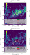 |
Fig. 2. Residual significance maps from the Fermi-LAT analysis in a zoomed region of the ROI. In the upper panel, the |

The four clouds were each detected with significant excesses and TS values of greater than 200. The exact values are summarised in Table 1. If a photon weighting procedure as used in the 4FGL catalogue (Abdollahi et al. 2020) is applied, the TS values are reduced but still greater than 150 for each cloud. The residual emission in the ROI could be clearly reduced with the addition of the cloud templates, as shown in Fig. 2. The remaining residual emission to the right side of the region could not be associated with molecular clouds in the CNC-Gum 31 complex (Rebolledo et al. 2016), but it might be connected to diffuse emission around Westerlund 2 (Yang et al. 2018). In order to account for it in the fit, an additional diffuse component based on the CO map by Dame et al. (2001) was introduced. The inclusion of this additional component helped improve the overall fit but did not affect the properties of the cloud components significantly. The spectra of the four individual clouds are shown in Fig. 3, and the best-fit spectral parameters are also included in Table 1. The spectral results with and without the photon weighting differ only by up to 0.04 for the spectral index and by 3% on the energy flux, and thus they are consistent within the statistical uncertainties. The values without the additional weighting were adopted, whereas the quoted differences could be interpreted as a contribution to the systematic uncertainty. For comparison, the spectrum of η Car is also shown in Fig. 3. The spectral shapes and normalisations determined for the Southern Cloud, Northern Cloud, and Gum 31 regions show a reasonable level of consistency, with a spectral index between 2.2 and 2.3. In contrast, the Southern Pillars are described by a slightly softer spectrum, mostly caused by an apparent cut-off above photon energies of 20 GeV. Below that energy, the derived flux points are comparable amongst all four clouds. Different spectral models for each cloud were tested by fitting the SEDs of each cloud separately. This yielded a difference of as much as 10% for the integrated energy flux, which can be considered as a contribution to the systematic uncertainty of the analysis.
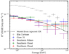 |
Fig. 3. Spectra of the four molecular clouds as derived from the Fermi-LAT analysis. For comparison, the spectrum derived for η Car is also shown in grey. Additionally, a model derived from an injected CR spectrum is shown. The CR spectrum was modelled as a power law with an index of 2.0 and an exponential cut-off at 2 TeV. The normalisation was scaled arbitrarily. |
Power-law spectral properties and TS values of the cloud templates.
The inner regions of the Carina Nebula are not resolvable with the current γ-ray instruments. For example, the Homunculus exists on scales corresponding to a factor 40 smaller than the 68% containment radius of the Fermi point spread function (PSF), which is ∼0.1° above 20 GeV (Abdollahi et al. 2020). An upper limit on the γ-ray flux originating from this inner region (but outside the WCR) can therefore only be estimated via the quiescent baseline component of the η Car γ-ray flux. Long-term light curves show only mild variability (e.g., W20; Martí-Devesa & Reimer 2021), with the γ-ray flux never dropping below 60% of the mean integrated flux level. This provides a baseline energy flux of (5.6 ± 0.3)×10−11 erg cm−2 s−1 integrated from 500 MeV to 100 GeV.
4. Propagation of CRs around η Car and expected emission
4.1. Particle acceleration and emission in the WCR
In this section, we summarise the relevant points of the model of O15 and W20 for CR production in the WCR (see also Eichler & Usov 1993; Bednarek & Pabich 2011). We then show how we used the model from W20 to obtain the spectrum of escaping CRs.
As mentioned in Sect. 2, the WCR contains two shocks. The wind of the more massive star η Car-A is slower (terminal wind speed v∞ ≈ 5 × 10² km s−1) and more dense (Ṁ ≈ 4.8 × 10⁻⁴ M⊙ yr−1) compared to that of the companion star η Car-B (v∞ ≈ 3 × 10³ km s−1, Ṁ ≈ 1.4 × 10⁻⁵ M⊙ yr−1, see Parkin et al. 2011). At the side of η Car-A, the high density leads to complete cooling of accelerated protons. The maximum proton energy is limited by inelastic collisions with compressed wind material, with Emax ∼ 200 GeV, and no energetic particles escape the acceleration region. On the side of η Car-B, the cooling time via collisions greatly exceeds the flow time, and accelerated particles can leave the acceleration region. W20 estimated that the maximum proton energy achievable at the wind termination shock of η Car-B is ≈30 TeV.
To match observations, approximately 10% of the wind power processed by each of the shocks should be converted into accelerated protons above 1 GeV. While energetic particles on the side of η Car-A are completely destroyed via hadronic collisions, on the side of η Car-B, particles can enter the ballistic region, that is, the flow transporting the shocked material laterally away from the WCR. The accelerated protons from the shock of η Car-B produce a non-negligible amount of γ-rays in the ballistic region as the shocked material from η Car-B mixes with the shocked higher density material from η Car-A. The amount of radiation produced depends on the details of the mixing process, which was adjusted in W20 to match the Fermi-LAT data. The number of interacting particles in the W20 model varies with the phase and is the largest at periastron.
For γ-rays produced in the wind region close to the stars, absorption due to pair production plays an important role. In this work, we restricted ourselves to the assumption of spherically symmetric emission. Due to the change in the stellar positions, there is an orbital variation in the absorption, in particular between phases 0.9 and 0.2. However, for emission on radial distance scales of 20 au, the phase dependence drops below 7% and decreases rapidly for emission on even larger scales.
In Fig. 1, the absorption for spherically symmetric emission at phase 0.5 for two different energies is shown. The case of 600 GeV corresponds roughly to maximum absorption. At 20 au, close to half of the emission is absorbed, whereas at 200 au, more than 90% of the γ-rays reach Earth. Thus, the VHE γ-ray emission reported by H.E.S.S. Collaboration (2020) can be more easily accounted for if it is produced at larger radii.
In the following, we use the average escaping CR spectrum and the stellar wind parameters quoted above, adapted from the model of W20, to investigate possible γ-ray emission produced by the escaping protons in the surrounding environment. Because the escaping proton spectrum in that work was not calculated directly, we inferred it by using the γ-ray data presented in W20. To obtain the spectral shape, we used the Naima package (Zabalza 2015) and assumed an exponential cut-off power-law proton spectrum. In the off-periastron phase range, this resulted in a power-law index of α ≈ 2 and a cut-off energy of Ecut ≈ 1.8 TeV. In W20, the γ-ray spectrum is calculated while the particles are advected with the flow out to a distance where the resulting emission is negligible and the radiative energy losses do not further change the underlying spectrum. We then assumed the spectrum of escaping particles to maintain the same shape. The proton spectrum above 1 GeV was then normalised such that the total energy in the escaping protons and transferred into γ-rays, the secondary particles and directly accelerated electrons is equal to the total power put into particle acceleration. Approximately 90% of the accelerated protons at the side of η Car B escape from the WCR.
4.2. Propagation in the wind region
The energetic particles that escape in the ballistic flow eventually merge with the winds. To avoid substantial adiabatic losses, the transport of these particles should be diffusion dominated. The ratio of the characteristic advection and diffusion timescales is a useful measure to determine which process dominates the radial transport:
 (1)
(1)
where u is the outward flow speed, Dr is the average radial diffusion coefficient, and R is the radial distance from the binary. Taking u ∼ 1000 km s−1 and R = 100 au, adiabatic losses can be neglected provided Dr ≫ 1023 cm2 s−1. While the radial diffusion coefficient is not known, the magnetic fields will be highly disordered in the ballistic region if the mixing is effective. This can, in principle, allow relativistic protons and other nuclei to decouple from the flow and escape the wind region without undergoing significant adiabatic losses.
If, on the other hand, particles were strongly coupled to the flow, the maximum energy would be reduced by adiabatic cooling: E ∝ ρ1/3 ∝ r−2/3. Thus, in crossing the wind region, the maximum particle energy would be reduced by a factor of ten or more. If the VHE measurements of H.E.S.S. Collaboration (2020) are produced far from the WCR, they provide a (model-dependent) constraint on the transport.
Protons that move outwards, either by diffusion or advection, remain in the low-density cavity evacuated by the wind from η Car-B, and they produce negligible γ-ray emission. However, some protons might migrate into the high-density wind from η Car-A and radiate significantly. If they remain in the high-density zone, they lose all of their energy due to hadronic interactions.
The spectrum of the protons migrating into the η Car-A wind depends on the transport processes, the details of which are currently not well constrained. In the most extreme case, when all protons penetrate into the wind of η Car-A, the energy in γ-rays detected on Earth using a total energy flux in escaping particles of 6.5 × 1035 erg s−1 from the model of W20 would be 10−9 erg cm s−1. This exceeds the flux detected by Fermi-LAT considerably, and the model parameters of W20 would have to be adapted. In the other extreme case, if a transport barrier exists at the interface of the two winds, excluding CRs from the denser target material, no significant emission would be produced in the wind region.
The variability of the γ-ray emission in the wind region is likely to be modest and not necessarily linked to the orbital phase, unless the γ-rays are produced only very close to the stars. Any potential emission from escaping protons in the wind region will thus contribute to an approximately steady baseline flux, modulo turbulent variations. The same should hold true for larger structures, such as the little and large Homunculus nebulae.
4.3. The little and large Homunculus nebulae
As shown in the previous section, only the particles diffusing in the low-density wind from η Car-B leave the pinwheel/wind region, and in the most extreme case, this could be the vast majority of the particles leaving the WCR. After the wind region, the CRs encounter the little Homunculus Nebula, which is likely to have a total mass of ∼0.1 M⊙ (Smith 2005). On larger scales, they encounter the > 10 M⊙ Homunculus Nebula (see Sect. 2). To obtain a rough estimate of the total γ-ray emission in each region, we used the following approximation:
 (2)
(2)
where FEarth is the total energy flux on Earth, tcross is the time it takes for the particles to cross each region, tcool is the cooling time, Lesc is the total energy in escaping particles, and d = 2.3 kpc is the distance towards η Car. For Lesc, we adopted the value of 6.5 × 1035 erg s−1 from the model of W20, assuming that energy losses are negligible in the pinwheel/wind region. We modelled the little Homunculus and the inner and outer shells of the large Homunculus as spherical shells around the stars for simplicity. We first considered the case of no diffusion within these thin shells, with CRs simply passing through at (close to) the speed of light.
Smith (2005) estimated the thickness of the little Homunculus to be ∼940 au. Using an average inner radius of 4 × 10³ au, a shell thickness of 1000 au, and a mass of 0.1 M⊙, the cooling time at 1 GeV is ∼4 × 10⁵ d. If the CRs move through the region with the speed of light, the resulting total energy flux on Earth is FEarth = 1.4 × 10⁻¹⁴ erg cm s−3. This is orders of magnitude below the energy flux from Fermi-LAT of 5.6 × 10⁻¹¹ erg cm s−3. The inner shell of the large Homunculus contains 10% of the total Homunculus mass (Smith 2006), which is between 1 M⊙ and 3.4 M⊙. To model it as a shell, we assumed an inner radius of 1 × 10⁴ au and an outer radius of 1.5 × 10⁴ au. For a mass of ∼2 M⊙, the resulting FEarth is 3.7 × 10⁻¹⁴ erg cm s−3. Different values of the inner and outer radius of the shell give similar results. For the outer Homunculus shell with an assumed density of 1.0 × 107 cm−3 and a thickness of 600 au, one obtains FEarth = 6.2 × 10⁻¹³ erg cm s−3. The outer Homunculus shell is therefore the most important region for the production of γ-rays by the escaping particles with fluxes at least one order of magnitude above the fluxes from the little Homunculus and the inner Homunculus shell. However, if the CRs pass through the outer shell at the speed of light, the γ-ray emission produced is still two orders of magnitude below the Fermi-LAT flux.
The Weigelt knots, located closer to the binary, have not been explicitly considered in this study. Adopting the typical Weigelt knot parameters from Remmen et al. (2013), the knots do not appear to have a sufficiently high overdensity relative to the parameters adopted for the Homunculus Nebula to make a significant difference to the γ-ray luminosity on those scales.
Cosmic rays are more likely to diffuse slowly through these shells of material than pass through at the speed of light. The outer Homunculus shell is the most massive and the most dense of the three shells, with likely larger magnetic fields and slower diffusion, and is hence expected to also dominate in this case. We therefore restricted the following calculations for different diffusion coefficients to emission from the outer shell. For simplicity, we ignored possible spectral changes caused by the propagation through the wind region, the little Homunculus, and the inner Homunculus shell because the exact propagation properties are unknown and are impossible to separate observationally from spectral changes by the propagation through the Homunculus itself. As before, we adopted a value of 1.0 × 107 cm−3 for the density in the outer shell. A lower limit on the (parallel) diffusion coefficient can be estimated by assuming Bohm diffusion. Unfortunately, the magnetic field in the shell is unknown and difficult to constrain. Values of 100 μG or even higher have been proposed (Aitken et al. 1995). To provide some numerical estimates, we took the energy dependence of the radial diffusion coefficient to have the following form:
 (3)
(3)
The dotted blue curve in Fig. 4 shows the emission produced in the Homunculus for D0 = 9 × 1022 cm2 s−1 and α = 0.5. As can be seen, interactions in the Homunculus Nebula of escaping CRs could produce a significant amount of steady γ-ray emission. Thus, models in which particle acceleration at the shock of η Car-A is ineffective, for example, due to a low Mach number or a highly oblique magnetic field, can be replaced with models in which the lower energy γ-rays are principally produced in the Homunculus. In Fig. 4, the red curve shows the emission produced by particles accelerated at the shock of η Car-B from the model of W20; the dashed red line is without absorption. The black dashed-dotted line shows this emission added to the emission from the Homunculus shown in the blue dashed-dotted curve for D0 = 9 × 1021 cm2 s−1, α = 1, and a factor of 1.1 more escaping CRs compared to the model of W20. The combined emission reproduces well the Fermi-LAT data over the whole energy range. In such a scenario, the weak phase-dependent variability is entirely produced by changes in the emission from η Car-B close to the binary. The assumed diffusion coefficient in the Homunculus is well above the case of Bohm diffusion for a magnetic field of 100 μG.
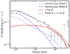 |
Fig. 4. Model of emission from η Car and the Homunculus together with Fermi-LAT data. The blue curves show emission from the Homunculus for different diffusion properties of the escaping CRs. The dotted curve (Model A) is for D0 = 9 × 1022 cm2 s−1 and α = 0.5. The dashed-dotted curve (Model B) is for D0 = 9 × 1021 cm2 s−1, α = 1, and a factor of 1.1 more escaping CRs compared to the model from W20. The red solid line shows the emission from η Car produced by particles accelerated at the shock towards η Car-B from W20 (the red dashed line is without absorption). The black dashed-dotted curve shows the combined emission from η Car-B and Model B. |
The above model consisting of particle acceleration occurring solely at the companion shock together with steady emission from the Homunculus by the escaping CRs can also account for the hard non-thermal X-ray emission. In the model of W20 the hard X-rays, similar to the γ-rays, are dominated by particles accelerated at the shock of η Car-B. Since that model reproduced the variability, we focus here on the phase averaged emission (see also Breuhaus 2022). While the orbital variability in the γ-ray emission shows energy-dependent behaviour that differs between orbits (Balbo & Walter 2017; Martí-Devesa & Reimer 2021), observations are nevertheless consistent with at least 60% of the emission being produced by a steady-state source. Using the existing γ-ray data, it is difficult to conclude which of these components dominates the quasi-steady emission, for example, emission produced near the wind termination shock of η Car-A (W20, Balbo & Walter 2017) or that which is produced on larger scales as presented here (see also Ohm et al. 2010; Skilton et al. 2012, for additional large scale sources). An observation of a reduction of the steady part of the emission or a clearly different behaviour in different energy bands could potentially constrain the possible contribution of the Homunculus Nebula and the wind region to the γ-ray flux, though the latter could equally be explained by the turbulent behaviour during the periastron passage, as suggested by Martí-Devesa & Reimer (2021).
5. Propagation in the Carina Nebula
Cosmic rays that escape both η Car and the Homunculus Nebula eventually enter the Carina Nebula. There they encounter the molecular clouds described in Sect. 2 as potential target material for further γ-ray production. The clouds of the CNC and Gum 31 exhibit significant γ-ray emission (see Sect. 3) that could be related to η Car. Figure 3 contains a model γ-ray spectrum derived from an injected CR distribution following a power-law with an exponential cut-off. In the models of O15 and W20, a non-linear diffusive shock acceleration model was used to account for the required hard underlying proton spectrum (see Sect. 4.1). The assumed CR spectrum has an index of 2.0 and an exponential cut-off at 2 TeV. To compute a γ-ray spectrum, the parametrisations from Kappes et al. (2007) were employed, and energy-dependent propagation leading to a softening of −1/3 was assumed. The resulting γ-ray spectrum has a similar profile to that measured by Fermi-LAT. The CR density in a certain region can be calculated from the γ-ray luminosity and cloud mass following the approximation given in Aharonian et al. (2019):
 (4)
(4)
Here, the parameter η accounts for the presence of heavier nuclei and is assumed to be 1.5. The γ-ray luminosity, Lγ, above 500 MeV is derived from integrating the γ-ray flux and assuming a typical distance of 2.3 kpc (i.e., the same as η Car). This translates into a minimum CR energy of 5 GeV. The masses are assumed to follow the dust mass estimate from Rebolledo et al. (2016), whose Table 2 is based on Herschel infrared Galactic Plane Survey (HiGAL; Molinari et al. 2010) data. The mass uncertainty derived from dust maps is mostly dominated by uncertainties in temperature derivation (∼10%; Urquhart et al. 2018), the HiGAL survey flux (∼5%; Molinari et al. 2016), and the local gas-to-dust mass ratio assumption. According to Giannetti et al. (2017), the local variation of this ratio is on order of 20%. Hence, we adopted an overall uncertainty of 25% on the mass, not reflecting systematic uncertainties that are common to all of the clouds (which are likely much larger but do not impact the shape of the profile).
The resulting CR density profile can be seen in Fig. 5. The physical extent is visualised by the horizontal error bars as the minimum and maximum distance from η Car. The conversion to a physical distance scale assumes that all clouds are located in a plane at the same distance from the observer. Compared to the result obtained by Ge et al. (2022), the result from Gum 31 is consistent with their result for region B, whereas their region A centred at η Car comprises both the Southern Cloud and parts of the Northern Cloud and is hence not directly comparable.
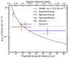 |
Fig. 5. Cosmic ray density for each of the four clouds as a function of distance to η Car. The angular distance was transformed into a physical distance using a distance to η Car of 2.3 kpc. Distance errors depict the maximum extent of the cloud templates. The 1/r type profile as described in Eq. (5) was fit to the data points and is shown by the dashed line. For comparison, the CR densities as derived in Ge et al. (2022) for their regions A and B are shown in light grey. |
Assuming η Car as the origin of the CRs suggests a 1/r profile, which is similar to that observed around some massive stellar clusters (Aharonian et al. 2019),
 (5)
(5)
Normalising the profile at r0 = 10 pc, a value of w0 = 0.48 ± 0.09 eV cm−3 in CRs above 5 GeV is obtained from a fit to the derived CR density profile. Using the maximum energy flux and mass for the Homunculus, as discussed above, provides an upper limit on the CR energy density of ∼103 eV cm−3 at a distance of ≲0.1 pc, which does not constrain the postulated 1/r behaviour. For an integration radius of 60 pc, corresponding to the outer edge of the emission seen in the CNC-Gum 31 complex, the derived CR energy density implies a total energy of CR protons of Wp = 5 × 1048 erg.
The diffusion time can be calculated from the maximum distance, Rmax, that CRs have propagated for a given diffusion coefficient. Here, Rmax is taken to be 60 pc, and the energy-dependent diffusion is assumed to follow Eq. (3). Together with a total power of ∼5 × 1035 erg s−1 escaping η Car in CRs above an energy of 5 GeV as suggested by the model in W20 , this implies a diffusion coefficient of D0 = 5 × 1026 cm2 s−1. While this is slower than the average Galactic diffusion coefficient (3 × 1028 cm2 s−1), it is well above the lower limit of 5 × 1025 cm2 s−1 implied by the age of η Car (∼2 − 3 × 10⁶ years, Mehner et al. 2010), and so, at first sight, it appears reasonable.
However, this diffusion coefficient implies diffusion times through the clouds that are on the same scale as the lifetime of the diffusing protons. The diffusion time through the northern cloud for our estimated diffusion coefficient and a cloud diameter of 30 pc, estimated from the size of the CO template, is ∼1.4 × 10⁵ yr. The lifetime of the diffusing protons is approximately tcool = 3 × 10⁷n−1 yr (e.g., Hinton & Hofmann 2009), corresponding to ≈105 yr for a spherical cloud of mass 105 M⊙ (Rebolledo et al. 2016). Consequently, the thin target approximation does not hold. Faster diffusion appears to be needed, leading to a higher total CR power that cannot be produced exclusively from η Car in its current state. Therefore, either the CR output from η Car was higher in the past by at least a factor of a few times its current value or a contribution from additional sources in the CNC is needed. Though η Car is known to be a highly variable system on timescales of ∼100 yr, little is known about the system prior to the great eruption in the 19th century. At the same time, several candidate sources exist that could contribute to the observed emission, including massive stellar clusters (such as the nearby Trumpler 14) and massive binaries situated in the star-forming regions of the CNC (Ge et al. 2022; Aharonian et al. 2019).
6. Summary and conclusion
In this work, we analysed Fermi-LAT data from η Car and four surrounding clouds and investigated CR escape, propagation, and γ-ray emission from the η Car binary system and its neighbourhood. The η Car system and its surroundings are extremely complex, with the wind region, little and large Homunculus nebulae, and molecular clouds nearby. For efficient escape of particles from the system, the CRs should diffuse in the low-density region carved by the wind from η Car-B; otherwise, they will either interact in the wind region or lose their energy via adiabatic losses. Particles diffusing into the high-density region can lead to an additional contribution to the total γ-ray spectrum. Depending on the propagation properties, the interaction of escaping particles in the Homunculus Nebula can account for a large fraction of the total γ-rays measured by Fermi-LAT.
We find the observed emission of η Car on scales not yet resolvable by Fermi-LAT can be accounted for by a variety of different models. In addition to what was put forward by W20, this also includes models solely accelerating particles at the shock on the η Car-B side, with the lower energy Fermi-LAT emission dominantly produced in the Homunculus (see Sect. 4). Therefore, it is possible that several zones contribute to the overall emission, a fact that should be included in any future model. However, the determination of the exact amount of emission produced in each region depends on the details of the CR transport and remains a challenge.
Escaping CRs from η Car may also interact in the molecular clouds of the Carina Nebula. As shown in Sect. 5, the derived radial profile of the CR densities seems to be indicative of an origin of CRs from η Car. However, to account for the current emission associated with molecular clouds, either η Car must have been more powerful in the past or additional CR sources must be present in the region (as proposed by Ge et al. 2022).
Observations of η Car at several hundreds of GeV and TeV energies by the Imaging Atmospheric Cherenkov Telescopes are also of great interest. This part of the spectrum is affected by absorption and potential adiabatic losses. Accurate and potentially time-dependent observations around periastron therefore help in the investigation of the propagation properties close to the stars as well as in constraining the emission regions. Observations from the H.E.S.S. telescopes of the most recent periastron passage and observations from the future CTA Observatory may provide crucial information to help unravel the physics of the fascinating binary system η Car.
Acknowledgments
For the numerical calculations in Sect. 4 we made use of the open-source code GAMERA (Hahn 2015; Hahn et al. 2022). To estimate the shape of the escaping proton spectrum, the Naima package was used (Zabalza 2015).
References
- Abdo, A. A., Ackermann, M., Ajello, M., et al. 2010a, ApJS, 188, 405 [NASA ADS] [CrossRef] [Google Scholar]
- Abdo, A. A., Ackermann, M., Ajello, M., et al. 2010b, ApJ, 723, 649 [NASA ADS] [CrossRef] [Google Scholar]
- Abdollahi, S., Acero, F., Ackermann, M., et al. 2020, ApJS, 247, 33 [Google Scholar]
- Abdollahi, S., Acero, F., Ackermann, M., et al. 2022a, ApJ, 933, 204 [NASA ADS] [CrossRef] [Google Scholar]
- Abdollahi, S., Acero, F., Baldini, L., et al. 2022b, ApJS, 260, 53 [NASA ADS] [CrossRef] [Google Scholar]
- Aharonian, F., Yang, R., & de Oña Wilhelmi, E. 2019, Nat. Astron., 3, 561 [Google Scholar]
- Aitken, D. K., Smith, C. H., Moore, T. J. T., & Roche, P. F. 1995, MNRAS, 273, 359 [NASA ADS] [CrossRef] [Google Scholar]
- Aydi, E., Sokolovsky, K. V., Chomiuk, L., et al. 2020, Nat. Astron., 4, 776 [CrossRef] [Google Scholar]
- Balbo, M., & Walter, R. 2017, A&A, 603, A111 [NASA ADS] [CrossRef] [EDP Sciences] [Google Scholar]
- Bednarek, W., & Pabich, J. 2011, A&A, 530, A49 [NASA ADS] [CrossRef] [EDP Sciences] [Google Scholar]
- Breuhaus, M. 2022, Dissertation, Ruprecht-Karls-Universität Heidelberg, Germany [Google Scholar]
- Bruel, P., Burnett, T. H., Digel, S. W., et al. 2018, arXiv e-prints [arXiv:1810.11394] [Google Scholar]
- Churchwell, E., Bieging, J. H., van der Hucht, K. A., et al. 1992, ApJ, 393, 329 [NASA ADS] [CrossRef] [Google Scholar]
- Clementel, N., Madura, T. I., Kruip, C. J. H., Icke, V., & Gull, T. R. 2014, MNRAS, 443, 2475 [NASA ADS] [CrossRef] [Google Scholar]
- Contreras, M. E., & Rodríguez, L. F. 1999, ApJ, 515, 762 [CrossRef] [Google Scholar]
- Dame, T. M., Hartmann, D., & Thaddeus, P. 2001, ApJ, 547, 792 [Google Scholar]
- Damineli, A., Hillier, D. J., Corcoran, M. F., et al. 2008, MNRAS, 384, 1649 [NASA ADS] [CrossRef] [Google Scholar]
- del Palacio, S., García, F., De Becker, M., et al. 2023, A&A, 672, A109 [NASA ADS] [CrossRef] [EDP Sciences] [Google Scholar]
- Dougherty, S. M., & Williams, P. M. 2000, MNRAS, 319, 1005 [NASA ADS] [CrossRef] [Google Scholar]
- Eichler, D., & Usov, V. 1993, ApJ, 402, 271 [Google Scholar]
- Farnier, C., Walter, R., & Leyder, J. 2011, A&A, 526, A57 [NASA ADS] [CrossRef] [EDP Sciences] [Google Scholar]
- Ge, T.-T., Sun, X.-N., Yang, R.-Z., Liang, Y.-F., & Liang, E.-W. 2022, MNRAS, 517, 5121 [NASA ADS] [CrossRef] [Google Scholar]
- Giannetti, A., Leurini, S., König, C., et al. 2017, A&A, 606, L12 [NASA ADS] [CrossRef] [EDP Sciences] [Google Scholar]
- Gould, R. J., & Schréder, G. P. 1967, Phys. Rev., 155, 1404 [Google Scholar]
- H.E.S.S. Collaboration (Abdalla, H., et al.) 2020, A&A, 635, A167 [NASA ADS] [CrossRef] [EDP Sciences] [Google Scholar]
- Hahn, J. 2015, Int. Cosmic Ray Conf., 34, 917 [NASA ADS] [Google Scholar]
- Hahn, J., Romoli, C., & Breuhaus, M. 2022, Astrophysics Source Code Library [record ascl:2203.007] [Google Scholar]
- Hamaguchi, K., Corcoran, M. F., Pittard, J. M., et al. 2018, Nat. Astron., 2, 731 [CrossRef] [Google Scholar]
- Hillier, D. J., Davidson, K., Ishibashi, K., & Gull, T. 2001, ApJ, 553, 837 [NASA ADS] [CrossRef] [Google Scholar]
- Hinton, J. A., & Hofmann, W. 2009, ARA&A, 47, 523 [NASA ADS] [CrossRef] [Google Scholar]
- Kappes, A., Hinton, J., Stegmann, C., & Aharonian, F. A. 2007, ApJ, 656, 870 [NASA ADS] [CrossRef] [Google Scholar]
- Madura, T. I., Gull, T. R., Owocki, S. P., et al. 2012, MNRAS, 420, 2064 [NASA ADS] [CrossRef] [Google Scholar]
- Madura, T. I., Gull, T. R., Okazaki, A. T., et al. 2013, MNRAS, 436, 3820 [NASA ADS] [CrossRef] [Google Scholar]
- Marcote, B., Callingham, J. R., De Becker, M., et al. 2021, MNRAS, 501, 2478 [NASA ADS] [CrossRef] [Google Scholar]
- Martí-Devesa, G., & Reimer, O. 2021, A&A, 654, A44 [NASA ADS] [CrossRef] [EDP Sciences] [Google Scholar]
- Martí-Devesa, G., Reimer, O., Li, J., & Torres, D. F. 2020, A&A, 635, A141 [Google Scholar]
- Mehner, A., Davidson, K., Ferland, G. J., & Humphreys, R. M. 2010, ApJ, 710, 729 [NASA ADS] [CrossRef] [Google Scholar]
- Mehner, A., Davidson, K., Humphreys, R. M., et al. 2015, A&A, 578, A122 [NASA ADS] [CrossRef] [EDP Sciences] [Google Scholar]
- Molinari, S., Swinyard, B., Bally, J., et al. 2010, PASP, 122, 314 [Google Scholar]
- Molinari, S., Schisano, E., Elia, D., et al. 2016, A&A, 591, A149 [NASA ADS] [CrossRef] [EDP Sciences] [Google Scholar]
- Moran, J. P., Davis, R. J., Bode, M. F., et al. 1989, Nature, 340, 449 [NASA ADS] [CrossRef] [Google Scholar]
- Nolan, P. L., Abdo, A. A., Ackermann, M., et al. 2012, ApJS, 199, 31 [Google Scholar]
- North, J. R., Tuthill, P. G., Tango, W. J., & Davis, J. 2007, MNRAS, 377, 415 [NASA ADS] [CrossRef] [Google Scholar]
- Ohm, S., Hinton, J. A., & Domainko, W. 2010, ApJ, 718, L161 [NASA ADS] [CrossRef] [Google Scholar]
- Ohm, S., Zabalza, V., Hinton, J. A., & Parkin, E. R. 2015, MNRAS, 449, L132 [NASA ADS] [CrossRef] [Google Scholar]
- Parkin, E. R., & Pittard, J. M. 2008, MNRAS, 388, 1047 [Google Scholar]
- Parkin, E. R., Pittard, J. M., Corcoran, M. F., & Hamaguchi, K. 2011, ApJ, 726, 105 [CrossRef] [Google Scholar]
- Preibisch, T., Ratzka, T., Kuderna, B., et al. 2011, A&A, 530, A34 [NASA ADS] [CrossRef] [EDP Sciences] [Google Scholar]
- Rebolledo, D., Burton, M., Green, A., et al. 2016, MNRAS, 456, 2406 [Google Scholar]
- Reitberger, K., Reimer, O., Reimer, A., et al. 2012, A&A, 544, A98 [NASA ADS] [CrossRef] [EDP Sciences] [Google Scholar]
- Reitberger, K., Reimer, A., Reimer, O., & Takahashi, H. 2015, A&A, 577, A100 [NASA ADS] [CrossRef] [EDP Sciences] [Google Scholar]
- Remmen, G. N., Davidson, K., & Mehner, A. 2013, ApJ, 773, 27 [CrossRef] [Google Scholar]
- Skilton, J. L., Domainko, W., Hinton, J. A., et al. 2012, A&A, 539, A101 [NASA ADS] [CrossRef] [EDP Sciences] [Google Scholar]
- Smith, N. 2005, MNRAS, 357, 1330 [CrossRef] [Google Scholar]
- Smith, N. 2006, ApJ, 644, 1151 [Google Scholar]
- Smith, N., & Ferland, G. J. 2007, ApJ, 655, 911 [NASA ADS] [CrossRef] [Google Scholar]
- Smith, N., Gehrz, R. D., Hinz, P. M., et al. 2003, AJ, 125, 1458 [NASA ADS] [CrossRef] [Google Scholar]
- Tavani, M., Sabatini, S., Pian, E., et al. 2009, ApJ, 698, L142 [NASA ADS] [CrossRef] [Google Scholar]
- Teodoro, M., Damineli, A., Heathcote, B., et al. 2016, ApJ, 819, 131 [Google Scholar]
- Urquhart, J. S., König, C., Giannetti, A., et al. 2018, MNRAS, 473, 1059 [Google Scholar]
- Vernetto, S., & Lipari, P. 2016, Phys. Rev. D, 94, 063009 [NASA ADS] [CrossRef] [Google Scholar]
- White, R., Breuhaus, M., Konno, R., et al. 2020, A&A, 635, A144 [NASA ADS] [CrossRef] [EDP Sciences] [Google Scholar]
- Wood, M., Caputo, R., Charles, E., et al. 2017, Proc. Int. Cosmic Ray Conf., 301, 824 [NASA ADS] [CrossRef] [Google Scholar]
- Yang, R.-Z., de Oña Wilhelmi, E., & Aharonian, F. 2018, A&A, 611, A77 [NASA ADS] [CrossRef] [EDP Sciences] [Google Scholar]
- Zabalza, V. 2015, Proc. Int. Cosmic Ray Conf., 34, 922 [Google Scholar]
Appendix A: Further Fermi-LAT analysis details
Configuration used for the Fermi-LAT analysis.
Appendix B: γγ-absorption
For the calculations of γγ-absorption in the anisotropic stellar radiation fields, we used the open-source GAMERA code (Hahn 2015; Hahn et al. 2022). It uses the standard cross-section for pair production, which can be found, for example, in Gould & Schréder (1967). In the form found in Vernetto & Lipari (2016, Eq. 1), the cross-section reads:
![Mathematical equation: $$ \begin{aligned} \sigma _{\gamma \gamma } = \sigma _{\rm T} \frac{3}{16} (1- \beta ^2)\left[2\beta (\beta ^2 -2) + (3-\beta ^4) \ln \frac{1+\beta }{1-\beta } \right], \end{aligned} $$](/articles/aa/full_html/2023/11/aa46483-23/aa46483-23-eq7.gif) (B.1)
(B.1)
where  with
with  and s = 2Eγϵ(1 − cos θ) the square of the centre-of-mass energy. Here, θ is the angle between the propagation directions of the two interacting photons, Eγ is the energy of the γ-ray photon, ϵ is the energy of the target photon, and me is the electron rest mass.
The propagation direction of the γ-ray photon is towards the observer, and the direction of the target photon depends on the position of the stars inferred from the orbital parameters. The eccentricity of the system was assumed to be 0.9 (Damineli et al. 2008), the semi-major axis is 16.64 au (Hillier et al. 2001), the inclination of the orbit is i = 135°, and the position angle is ϕ = 10° (Madura et al. 2012). For each star, which was modelled as a black body, Equation B.1 was integrated over the stellar surface, which is assumed to uniformly produce photons. This means that each point of the stellar surface produces the same amount of photons at the same temperature. The stellar temperatures are the same as in O15 and W20, 2.58 × 10⁴ K for the primary star and 3 × 10⁴ K for the companion.
Figure B.1 shows the transmissivity at 220 GeV, 620 GeV, and 4 TeV for different distances from the centre of mass of the system, assuming a spherical uniform γ-ray production. As can be seen in the figure, the transmissivity increases with increasing radius. This is expected due to the decreased radiation energy density at larger distances from the stars.
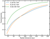 |
Fig. B.1. Transmissivity versus distance from the centre of mass of the binary system for spherical emission and different energies at an orbital phase of 0.5. |
At a distance of 25 au, the transmissivity at 220 GeV is larger than at 620 GeV. However, the opposite is the case for distances above ∼75 au. This is caused by the relative position of the two stars and their different temperatures. As η Car-B is hotter than η Car-A, it therefore has more impact at lower energies than at higher energies. The relative absorption from each star changes with different radii because of the stellar separation, which is slightly more than 30 au, and because the centre of mass of the system is around five times more distant from η Car-B than from η Car-A. The relative absorption by target photons from η Car-B compared to η Car-A increases with distance for the apastron position, creating the observed effect for the curves at 220 GeV and 620 GeV.
All Tables
All Figures
|
Fig. 1. Scales relevant to the possible emission regions around η Car. Because some regions, such as the large and the little Homunculus nebulae, are asymmetric or have sizes that can change over time, such as for the shock cap, the sizes shown cover a large range of values. The different extensions are as follows: 1–20 au (shock cap, A); 10–6.4 × 10³ au (wind region, B); 2 × 10³ to 6.5 × 10³ au (little Homunculus, C); 2.1 × 10³ to 21.69 × 10³ au (Homunculus, D); and > 50 × 103 au (Carina Nebula, E). The black and grey bars in the upper-left corner indicate the distances beyond which the absorption at 200 GeV is less than 50% (black) and the absorption at 600 GeV is less than 10% (grey), see text for more details. The individual images are from Parkin et al. (2011), Clementel et al. (2014), Smith (2005), HST, and ESO. |
| In the text | |
|
Fig. 2. Residual significance maps from the Fermi-LAT analysis in a zoomed region of the ROI. In the upper panel, the |
| In the text | |
|
Fig. 3. Spectra of the four molecular clouds as derived from the Fermi-LAT analysis. For comparison, the spectrum derived for η Car is also shown in grey. Additionally, a model derived from an injected CR spectrum is shown. The CR spectrum was modelled as a power law with an index of 2.0 and an exponential cut-off at 2 TeV. The normalisation was scaled arbitrarily. |
| In the text | |
|
Fig. 4. Model of emission from η Car and the Homunculus together with Fermi-LAT data. The blue curves show emission from the Homunculus for different diffusion properties of the escaping CRs. The dotted curve (Model A) is for D0 = 9 × 1022 cm2 s−1 and α = 0.5. The dashed-dotted curve (Model B) is for D0 = 9 × 1021 cm2 s−1, α = 1, and a factor of 1.1 more escaping CRs compared to the model from W20. The red solid line shows the emission from η Car produced by particles accelerated at the shock towards η Car-B from W20 (the red dashed line is without absorption). The black dashed-dotted curve shows the combined emission from η Car-B and Model B. |
| In the text | |
|
Fig. 5. Cosmic ray density for each of the four clouds as a function of distance to η Car. The angular distance was transformed into a physical distance using a distance to η Car of 2.3 kpc. Distance errors depict the maximum extent of the cloud templates. The 1/r type profile as described in Eq. (5) was fit to the data points and is shown by the dashed line. For comparison, the CR densities as derived in Ge et al. (2022) for their regions A and B are shown in light grey. |
| In the text | |
|
Fig. B.1. Transmissivity versus distance from the centre of mass of the binary system for spherical emission and different energies at an orbital phase of 0.5. |
| In the text | |
Current usage metrics show cumulative count of Article Views (full-text article views including HTML views, PDF and ePub downloads, according to the available data) and Abstracts Views on Vision4Press platform.
Data correspond to usage on the plateform after 2015. The current usage metrics is available 48-96 hours after online publication and is updated daily on week days.
Initial download of the metrics may take a while.