| Issue |
A&A
Volume 635, March 2020
|
|
|---|---|---|
| Article Number | A144 | |
| Number of page(s) | 12 | |
| Section | Astrophysical processes | |
| DOI | https://doi.org/10.1051/0004-6361/201937031 | |
| Published online | 24 March 2020 | |
Gamma-ray and X-ray constraints on non-thermal processes in η Carinae
1
Max-Planck-Institut für Kernphysik, Postfach 103980, 69029 Heidelberg, Germany
e-mail: This email address is being protected from spambots. You need JavaScript enabled to view it.
; This email address is being protected from spambots. You need JavaScript enabled to view it.
2
DESY, 15738 Zeuthen, Germany
Received:
30
October
2019
Accepted:
7
January
2020
Abstract
The binary system η Carinae is a unique laboratory that facilitates the study of particle acceleration to high energies under a wide range of conditions, including extremely high densities around periastron. To date, no consensus has emerged as to the origin of the gigaelectronvolt γ-ray emission in this important system. With a re-analysis of the full Fermi-LAT data set for η Carinae, we show that the spectrum is consistent with a pion decay origin. A single population leptonic model connecting X-ray to γ-ray emission can be ruled out. We revisit our physical model from 2015, based on two acceleration zones associated with the termination shocks in the winds of both stars. We conclude that inverse Compton emission from in-situ accelerated electrons dominates the hard X-ray emission detected with NuSTAR at all phases away from periastron and that pion-decay from shock accelerated protons is the source of γ-ray emission. Very close to periastron there is a pronounced dip in hard X-ray emission, concomitant with the repeated disappearance of the thermal X-ray emission, which we interpret as due to the suppression of significant electron acceleration in the system. Within our model, the residual emission seen by NuSTAR at this phase can be accounted for with secondary electrons produced in interactions of accelerated protons, which agrees with the variation in pion-decay γ-ray emission. Future observations with H.E.S.S., CTA, and NuSTAR should confirm or refute this scenario.
Key words: radiation mechanisms: non-thermal / acceleration of particles / gamma-rays: stars / stars: individual: η Car / stars: winds / outflows / X-rays: binaries
© R. White et al. 2020
 Open Access article, published by EDP Sciences, under the terms of the Creative Commons Attribution License (https://creativecommons.org/licenses/by/4.0), which permits unrestricted use, distribution, and reproduction in any medium, provided the original work is properly cited.
Open Access funding provided by Max Planck Society.
1. Introduction
η Car is the most prominent γ-ray emitting colliding wind binary system, which is known to have many exceptional properties. The high mass-loss rates of the binary stars in this system lead to very high densities in the wind collision region (WCR), which may in turn lead to efficient conversion of energy from accelerated protons into γ-rays and neutrinos. The orbit of the system is highly eccentric with an eccentricity above 0.8 and most likely between 0.85 and 0.90 (Mehner et al. 2015) and a period of ∼5.5 yr (Damineli et al. 2008), which results in very different conditions in a WCR over the course of a single orbit. The primary star of the system is believed to be a luminous blue variable (Davidson & Humphreys 1997) and the companion a late-type nitrogen-rich O or Wolf–Rayet star (Iping et al. 2005). Throughout the paper we refer to the primary star as η Car A and to the companion star as η Car B. η Car A has a mass larger than 90 M⊙ with an initial mass of probably 150 M⊙ or higher. The mass of η Car B is also not well known, but should be not larger than 30 M⊙ (Hillier et al. 2001). Their winds have different properties: the mass-loss rate of η Car A was estimated to be a few 10−4 M⊙ yr−1 up to a few 10−3 M⊙ yr−1 and the terminal wind velocity to be ≈500 km s−1; for η Car B possible values are around 10−5 M⊙ yr−1 and ≈3000 km s−1 (see Corcoran & Hamaguchi 2007, and references therein). The surface magnetic-field strengths of the stars are uncertain. In discussing the radio measurements of WR147 made by Williams et al. (1997) and Walder et al. (2012) conclude that the emission is consistent with surface magnetic-field strengths of 30–300 G.
The variability of η Car is well studied in the X-ray domain (see e.g. Corcoran 2005; Hamaguchi et al. 2007, 2014). An outline of the X-ray measurements between 1996 and 2014 is given in Corcoran et al. (2015) and put in perspective with the orbital dynamics of the system. The X-ray maximum is explained by a wind-wind cavity carved in the dense wind of η Car A due to the motion of the companion η Car B and its stellar wind. The X-ray minimum follows as a consequence of the subsequent blocking of the said cavity in further companion motion.
The first detections of γ-ray emission from the direction of η Car were obtained with the Astro-Rivelatore Gamma a Immagini Leggero (AGILE) satellite (Tavani et al. 2009) and Fermi Large Area Telescope (Fermi-LAT; Abdo et al. 2009, 2010). The γ-ray flux is observed to vary around the orbit; this flux has an increase shortly before and a decrease around periastron (Abdo et al. 2010; Farnier et al. 2011), albeit less significantly than in the X-ray regime. The γ-ray spectrum measured using Fermi-LAT can be described well by two different components, one of which dominates the emission above 10 GeV (Abdo et al. 2010; Farnier et al. 2011). Farnier et al. (2011) suggested that the low-energy component may be associated with inverse Compton (IC) scattering by electrons accelerated in the WCR, and the second component may be from decay of π0s produced in the interactions of accelerated hadrons in the dense environment.
Bednarek & Pabich (2011) were the first to suggest that the two shocks in the system, owing to the different stellar wind properties for the individual stars, would lead to two populations of accelerated particles with different maximum energies. These authors considered two different models: one solely containing accelerated electrons and the other both high-energy electrons and protons. In Ohm et al. (2015; hereafter O15) this scenario was explored further with a more complete treatment of the system geometry and dynamics. These authors concluded that the γ-ray emission is likely purely hadronic in origin and that the two Fermi-LAT components are indeed associated with the two shocks in the system.
The first full orbit of η Car as seen by Fermi-LAT was analysed by Reitberger et al. (2015). They found small variations at energies < 10 GeV, but larger variations for the high-energy component, with a high flux at periastron, followed by a sudden decrease and a slow recovery. With the updated Fermi-LAT coverage of two periastron passages and the major improvement in sensitivity (particularly at low energies) represented by the Pass 8 release of Fermi-LAT data, further information about the variability in the γ-ray regime has been presented by Balbo & Walter (2017). The high-energy component does not show a significant increase during the second observed periastron passage, but the low-energy component behaves in a similar way during both passages. Comparing their results with γ-ray fluxes derived from data of hydro-dynamical simulations of Parkin et al. (2011) and Balbo & Walter (2017) argued again in favour of a model in which the low-energy γ-ray emission is attributable to IC scattering.
Recently, Hamaguchi et al. (2018) have reported on observations with NuSTAR in the hard X-ray domain, which confirmed earlier suggestions (Leyder et al. 2008) of a hard, non-thermal, component at 30–50 keV. These authors contend that this is IC emission connecting smoothly with the low-energy component seen with Fermi-LAT, thereby inferring that hard X-ray emission and low-energy γ-ray emission are produced by the same population of relativistic electrons.
We revisit the Fermi-LAT data, focussing on the previously unconstrained lowest energy (< 200 MeV) part of the γ-ray spectrum with the aim of constraining the origin of this component (Sect. 2). In Sect. 3 we make an assessment of the likely origin of various non-thermal components of η Car based on physical considerations associated with particle acceleration, energy losses, and the emission and absorption of γ-rays. In Sect. 4 we present an update of the calculation of O15 and a comparison to the newly available data. Finally, in Sect. 5 we discuss the implications of the new data analysis and modelling and prospects for future observations.
2. Fermi-LAT data analysis
2.1. Data selection
We performed a Fermi-LAT analysis closely following the approach taken by Reitberger et al. (2015) but considering a wider energy range, additional data, an updated Galactic diffuse model, updated instrument response functions (IRFs) and the latest Fermi-LAT source catalogue.
Fermi-LAT data from the latest Pass 8 release between August 4 2008 and July 1 2019 (MET 239557417 to 583643061) was analysed using Fermitools (version 1.0.7), which is the official Fermi ScienceTools data-analysis suite1 via FermiPy (version 0.17.4), an open-source Python framework that provides a high level interface to the Fermi ScienceTools; (Wood et al. 2017).
Data were selected over a region of interest (ROI) of 10° by 10° centred at the nominal position of η Car and aligned in Galactic coordinates. Data were chosen according to the SOURCE event class (evclass=128) with FRONT+BACK event types (evtype=3).
To minimise contamination from atmospheric γ-rays from the Earth, time periods in which the ROI was observed at zenith angle greater than 90° were excluded and the resulting exposure correction determined as part of the live-time computation, as per the current Fermi-LAT recommendations2. A bright nova, ASASSN-18fv, approximately 1° away from η Car was detected by the Fermi-LAT in March 2018 (Jean et al. 2018). To prevent contamination at the position of η Car by emission from this nova, data in the period MET 542144904 to 550885992 were excluded.
2.2. Data analysis
The Fermi-LAT eight-year source catalogue (4FGL; Fermi-LAT Collaboration 2020) was used to construct a model of the sources surrounding η Car. To account for the instrument point spread function and any extended sources just outside the chosen ROI, sources from an extended region of radius 15° were included in the model. In total 63 sources were included. In all cases the spectral model was included as per the catalogue description. The latest Galactic diffuse background template and isotropic component files were utilised (see Appendix A for the specific files used). η Car was included as it appears in the 4FGL catalogue under the identifier 4FGL J1045.1−5940 as a point source with a log-parabolic spectral shape.
A binned maximum-likelihood analysis using the recommended IRFs was performed in the energy range 80 MeV−500 GeV. First the parameters of the background model were optimised in an iterative fashion, looping over all model components in the ROI fitting their normalisation and spectral shape parameters. Then a final fit was performed in which the Galactic and isotropic background components remain fixed whilst the normalisation of all sources within 3° of η Car with a test statistic (TS) > 10 and at least ten predicted events are allowed to vary. The TS and residuals maps were then generated to assess the quality of the model.
It was found that significant extended residual emission was present surrounding η Car after this process. These residuals resemble the distribution of molecular gas in the region, suggesting an additional component associated with cosmic-ray interactions in the region. A template spanning 1° radius based on the CO survey of Dame et al. (2001) was generated and added as a diffuse component to the overall model with a power-law spectral shape. The need for this additional diffuse component is discussed further in Appendix A. The best overall model fit then results in a TS of ∼1000 for the new component, which has a spectral index of 2.1 ± 0.1. The best-fit flux of this component is approximately 60% that of η Car. The mean velocity-integrated intensity in the CO template corresponds to a total gas mass of approximately 1 × 10⁵ M⊙ assuming a conversion factor of CO to molecular hydrogen (XCO) of 2 × 10²⁰ K km s−1 (consistent with studies for this region; cf. Rebolledo et al. 2015). The additional energy density in cosmic rays required to produce the energy flux of this component in γ-rays between 100 MeV and 30 GeV of 7 × 10⁻¹¹ erg cm−2 s−1 is ≈1 eV cm−3 over this ∼80 pc region. Whilst it is perhaps not surprising that the Galactic diffuse model used in Fermi-LAT cannot perfectly reproduce the emission from this complex region, this component is suggestive of an excess of locally accelerated cosmic rays in the region. Although a model with multiple templates allowing for different cosmic-ray densities in individual molecular clouds may more accurately represent the diffuse emission, the approach taken in this work results in an acceptably flat residuals map; this approach is hence justified for use in the analysis of η Car. The resulting model including this component was used as a starting point for the further analysis steps outlined below.
2.3. Spectral energy distribution
A spectral analysis of the full Fermi-LAT data set was performed based on the optimised model described above. The resulting spectral energy distribution (SED) together with systematic error band are shown in Fig. 1. Details of the systematic error estimate are provided in Appendix A.3. The SED for the total η Car data set from this work is consistent with that from Reitberger et al. (2015). A drop in flux below 300 MeV is clearly visible in the measured SED, which is indicative of a kinematic pion cut-off. The Naima package (Zabalza 2015) was used to fit the SED points under the assumption that the γ-ray emission arises entirely from proton-proton interactions. The measured SED appears to be inconsistent with a purely leptonic scenario, such as that presented in Hamaguchi et al. (2018).
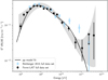 |
Fig. 1. Spectral energy distribution resulting from Fermi-LAT analysis of η Car over the full data set (black points) together with a systematic error band (grey area). A fit to the data points below 200 GeV using the Naima package (Zabalza 2015) is shown by the black curve under the assumption that the γ-ray emission arises from proton-proton interactions with an exponential cutoff power-law distribution for the protons. Data points from a previous Fermi-LAT analysis (Reitberger et al. 2015) are shown in blue for comparison. |
2.4. Phase-resolved SED analysis
The Fermi-LAT data on η Car spans 11 years covering two periastron passages over a relative phase range from 0.92 to phase 2.88. We produced SEDs for the following phase ranges motivated by the X-ray behaviour:
-
Pre-periastron: Phase ranges 0.92–0.99 and 1.92–0.99 (approximately 140 days each) covering the gradual build up in flux observed in the X-ray light curve.
-
Periastron: Phase ranges 0.995–1.025 (approximately 60 days each) covering the abrupt dip in flux observed in the X-ray light curve.
-
Off-periastron: Phase ranges 1.1–1.9 and 2.1–2.88, excluding 2.65–2.70 for the nova, ASASSN-18fv (Jean et al. 2018) where no significant variability is observed in the X-ray light curve.
In each phase range a fit was performed starting from the optimised model in which the Galactic and isotropic background components remain fixed to the previous optimised values. The normalisation of all sources within 3° of η Car with a TS > -pagination 10 and at least ten predicted events were allowed to vary. The analysis was performed both independently for each orbital period and with both orbital periods combined. The SEDs from the combined analysis of both orbits are presented in Sect. 3 and compared to those from the individual orbital periods in Appendix A.4.
2.5. Temporal analysis
The upper panel of Fig. 2 shows the light curve around periastron for the Fermi-LAT data in the energy range 300 MeV − 10 GeV divided into 0.03 bins in orbital phase (approximately 60 days) and aligned to the periastron phase range used in the SED analysis described in the previous section. The light curve was produced by performing an independent likelihood analysis in each time bin starting from the optimised model described in Sect. 2.2. In each time bin only nearby source normalisations and the normalisation of η Car were allowed to vary. An energy range from 300 MeV to 10 GeV, in which the spectral shape of η Car is roughly constant, was chosen. Data from the first orbital period observed by Fermi-LAT (with periastron in 2009) are shown in blue whilst data from the second orbital (periastron 2015) are shown in black. For comparison the points from Balbo & Walter (2017) are included. Hard X-ray emission as measured by NuSTAR during the 2014 periastron passage (Hamaguchi et al. 2018) is shown in the middle panel. In the lower panel X-ray emission at lower energies as measured by RXTE and Swift for passages culminating with periastron in 1998, 2003, 2009 and 2014 are shown (Corcoran et al. 2017). The 300 MeV − 10 GeV γ-ray flux behaves similarly during both passages (as noted by Balbo & Walter 2017) and shows no distinct disappearance at periastron as seen in the X-ray data.
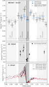 |
Fig. 2. Upper panel: Fermi-LAT temporal analysis of η Car from 300 MeV to 10 GeV from orbital phase 0.8 to 1.2 in 0.03 phase bins. Data corresponding to the first orbital period observed by the Fermi-LAT (with periastron in 2009) are shown in blue, and those corresponding to the second orbital period (with periastron in 2014) in black. Vertical grey shaded areas indicate the phase ranges used in the spectral analysis presented in Sect. 2.4 around periastron, pre-periastron, and off-periastron. The points from Balbo & Walter (2017) are shown as hollow grey circles. The vertical black dashed line indicates periastron. Middle panel: NuSTAR points for the 2014 periastron passage from Hamaguchi et al. (2018). Lower panel: RXTE and Swift data for the last four periastron passages. |
3. Physical considerations and limits
Before describing the numerical model, many important conclusions can be drawn about the significant effects and likely origin of different radiation components in the η Car system. From estimates of stellar luminosities, mass-loss rates, wind velocities, and surface magnetic fields, order of magnitude estimates of the conditions at the two shocks within the system can be derived and associated acceleration and energy-loss timescales considered. In this section we consider in turn each of the primary physical processes at work in the system, which have implications for non-thermal emission.
Following Bednarek & Pabich (2011), we consider the WCR separated from the winds of the two stars on either side by shock fronts. Despite the large densities, both shocks are collisionless (Hall parameter ωgiτii of the order 105 or larger; cf. Eichler & Usov 1993), and in principle provide sites for the acceleration of energetic particles via diffusive shock acceleration. The conditions pertinent to this process are discussed below.
3.1. Acceleration at η Car A shock
The inferred high surface fields and terminal velocity of the wind of η Car A limits the Alfvén Mach number of the shock to rather modest values, MA < 10, reaching a minimum near periastron. At all phases, the inferred low Mach numbers restrict the amount of self-generated MHD fluctuations that in situ accelerated particles can amplify upstream of the shock. From energy conservation, we must satisfy δB2/4π = χPcr, where Pcr is the cosmic-ray pressure and χ ≪ 1 the fraction that is converted to magnetic pressure. Re-arranging this equation as
 (1)
(1)
and using the results of Bell (2004), where χ ≈ vsh/c, we find only modest growth of magnetic fluctuations (δB ≲ B0) is possible. In the most optimistic scenario, the Hillas limit (Hillas 1984) for the shock of η Car A is (neglecting losses) written as
where R⋆ and B⋆ are the stellar radius and surface magnetic field, respectively, L ≈ rshθA is the spatial extent of the shock, and for convenience we have taken a purely toroidal magnetic field in the wind, B ∝ r−1. However, as we show below, the maximum energy in η Car A is always limited by losses. We note that while significant magnetic-field amplification can be ruled out, the growth rate for the classical ion-cyclotron instability (e.g. Tademaru 1969) can be sufficiently rapid to ensure acceleration efficiency close to the Bohm limit.
3.2. Acceleration at η Car B shock
The faster wind of η Car B should result in large Alfvén Mach numbers. Making the reasonable assumption that the star rotates at < 10% of its critical velocity, the shock is quasi-parallel (< 45°) over its entire orbit. The Alfvén Mach number thus increases monotonically with distance from the star. Plausible stellar surface parameters and wind conditions imply Alfvén Mach numbers MA > 100, and consequently the possibility of non-linear magnetic-field amplification should be considered (cf. Eq. (1)).
An estimate for the maximum attainable energy can be found from the Hillas limit, assuming strong field amplification. In reality, the statistics of the fields play an important role, and the Hillas result should be considered as a firm upper limit. Adopting standard parameters for the saturated magnetic field (e.g. Bell 2004):  , χ = vB, ∞/c; the Hillas limit gives EHillas ≈ 30 TeV. Hence, η Car can be seen to provide a unique time-dependent laboratory for testing theories of cosmic-ray acceleration with self-amplified fields relevant to high Alfvén Mach number supernova remnant shocks for example. Conversely, as the resulting γ-ray emission is dependent on the physical characteristics of the stellar wind, the high-energy observations may provide new information on what is otherwise a poorly constrained star.
3.3. Electron heating and injection
The shock conditions close to periastron require special consideration, as the injection of electrons is sensitive to shock obliquity and Mach number. In the case of η Car A, the relatively modest Alfvén Mach number may restrict electron injection, unless the shock is highly oblique. Hence, electron acceleration may not occur close to the star, where the fields are predominantly radial. Close to periastron, the shock may even become sub-critical (Edmiston & Kennel 1986), which can also suppress electron heating.
At η Car B, again the situation is different, although electron acceleration may also be inhibited close to periastron. The fate of the shock close to periastron is unclear. For example, it has been argued that the shock of η Car B collapses onto its stellar surface during closest approach (e.g. Parkin et al. 2011), although this requires a very weak surface magnetic field. As we argue below, the sustained γ-ray emission requires persistence of the shock. Another factor that can affect the non-thermal electron spectrum concerns the fact that for quasi-parallel shocks, electron acceleration requires the shock velocity to exceed the whistler phase speed (Eichler & Usov 1993), i.e.  . Since MA ∝ r in the radial field zone, this condition is violated close to the star unless the surface fields are extremely weak.
3.4. Interactions of protons
Accelerated protons and nuclei inevitably interact with the thermal background particles, leading to the production of γ-rays, neutrinos, and secondary leptons, which may in turn produce X-rays and γ-rays via the IC process. For η Car A, the proton energy-loss timescale via such collisions at the stagnation point is approximately ten days, significantly shorter than the propagation timescales via advection or diffusion. This is therefore a calorimetric system, in which energy gained by acceleration is lost in situ and the maximum energy attainable can be estimated from equating the timescales for energy loss (tpp ≈ (ngasσppc)−1) and Diffusive Shock Acceleration (DSA)  as follows:
 (2)
(2)
For our assumed orbital parameters, and a constant acceleration efficiency of ηacc = 5, this gives mean values of ∼150 GeV, but the energies are always below 230 GeV. At the shock in the wind of η Car B, densities are much lower and velocities higher. The flow timescales are shorter than the energy-loss timescales and it seems plausible that the maximum energy is determined by the residence time of protons and nuclei in the acceleration region, potentially reaching its Hillas limit (e.g. Achterberg 2004). The fraction of these particles that interact rather than escape from the system is dependent on the details of the cosmic-ray transport out of the system and also on the way in which the material in the two very different stellar winds becomes mixed on larger scales (see also O15).
Proton interactions with photons are also possible, however, for the radiation fields of the stars, using the cut-off energies we expect in the system, the interaction is always below the threshold energies of photo-meson and photo-pair production (see e.g. Schlickeiser 2002). And while the threshold condition can be met from interaction with the IC photons, the intensity is too low to be of any consequence.
3.5. Electron cooling
In η Car, conditions are such that energy-loss timescales for relativistic electrons are always much shorter than orbital timescales or particle escape timescales. An equilibrium between particle acceleration and cooling is therefore rapidly established at all electron energies. The dominant cooling process at the lowest energies is through electronic excitation (Gould 1975), at higher energies IC losses dominate and finally for the highest-energy electrons Klein–Nishina suppression beyond ∼10 GeV energies leave synchrotron emission as the dominant cooling process (see Fig. 2 in O15). The transition point between Coulomb-Ionisation losses and IC cooling depends on the ratio of thermal electron density to radiation energy density. As both of these quantities vary as the inverse square of the distance to the star, this cross-over point is approximately constant with phase. Following Schlickeiser (2002) the transition occurs at electron energies of
 (3)
(3)
i.e. the break energy is 130 MeV for the side of η Car A and 30 MeV for η Car B. The subscript “A” in Eq. (3) refers to the properties of η Car A. More accurate calculations, including the radiation fields from both stars and averaging over phases, reduces these values to 110 MeV and 15 MeV, respectively. In equilibrium the electron spectrum in any case softens above this point, leading to a break in the resulting IC spectrum, which lies well below the Fermi-LAT energy range for any reasonable choice of parameters.
3.6. Anisotropy of IC emission
As the typically assumed situation of isotropy in both the electron and target photon populations is not met in η Car, it is important to evaluate the impact of anisotropy on the expected IC emission. The electrons can still be assumed to be isotropic, since the velocities of the non-thermal particles are much larger than the flow velocities. We therefore adopt the cross section of Aharonian & Atoyan (1981) for the anisotropic IC scattering of an isotropic electron distribution. We find that there is a general compensating effect when one accounts for the radiation fields of the two stars and the different locations in the shock cap, such that the impact of anisotropy on the flux is always less than 30% in the range 30–50 keV, where IC emission from electrons dominates and measurements from NuSTAR are available. Averaging over different phases reduces the impact of anisotropy even further.
3.7. γ–γ pair-production
Above a threshold of ∼30 GeV, γ-rays inside the η Car system can pair-produce in the stellar radiation fields. The angular-dependent effects lead to phase-dependent flux variability in the very high energy domain. In the core energy of Fermi-LAT around 1 GeV γ − γ absorption is negligible. In our detailed model, described in the next section, we consider γ − γ pair-production only as an absorption process. In this section, however, we note that the presence of a significant flux of γ-rays beyond 30 GeV inside the system may result in a measurable contribution to the IC emission from the resulting pairs (see e.g. Dubus 2006; Bosch-Ramon & Khangulyan 2009). The IC emission of the pair-produced particles is expected to peak between 5 and 10 GeV and results in an enhancement of ∼10% close to periastron because of the proximity of the stars and the smaller size of the emission region. At all other phases the enhancement is less than 1%.
4. Phase-dependent model
To model non-thermal emission of η Car as a function of phase we made use of the framework presented in O15; we made some refinements and adjustment of parameters for consistency with the new full Fermi-LAT data set as described above. We adopted values for the wind and stellar parameters from the literature, whcih are summarised in Table 1. We note that while these parameters are not precisely constrained from observations, significant variation is not expected (with the exception of the surface magnetic-field strength). In this regard, the results that follow can be taken to be accurate with a similar level of confidence as our knowledge of the properties of the stars and their winds. This follows since, on fixing the other model parameters, the acceleration efficiency and the fraction of power dissipated into accelerated particles are both constrained by matching the position of the measured spectral breaks (see Sect. 3) and flux normalisation. High precision temporal and spectral gamma-ray measurements may thus be used to constrain the stellar parameters, complementing observations in longer wavelength regimes.
Adopted model parameters associated with the two stars in the η Car system and their associated wind shocks.
4.1. Modelling approach
We model diffusive shock acceleration at the two shocks in the system, forming on either side of the contact discontinuity between the two stellar winds (Eichler & Usov 1993). We assume constant and spherically symmetric winds; the geometry of the shock cap is established by the momentum balance between the two winds (see Canto et al. 1996, or Pittard & Dawson 2018 for the more general result). The parameters of the two stars and their winds are given in Table 1. For simplicity the winds of both stars are taken to be at their terminal velocities before reaching the shocks, although close to periastron we note that this approximation is inaccurate. For a v(r) = v∞(1 − R/r) β profile (Castor et al. 1975), with β = 1, a reduction in the shock velocities of 40% and 18% is expected at η Car A and B, respectively. Acceleration is assumed to take place with Bohm scaling (mean free path proportional to gyroradius) using the scaling factor ηacc, which is a free parameter of the model. The above-mentioned reductions in the shock velocity can be offset by a change in this parameter. Again for simplicity, we have kept both these numbers phase-independent.
We mimic the effect of magnetic-field amplification at the shock in the wind of η Car B by adopting a large rotation velocity. That this is reasonable follows from Eq. (1), where we can see that for constant acceleration efficiency, the amplified field corresponds to δB2 ∝ ρ. Provided anisotropic transport is unimportant, which is implicitly assumed in the model, the magnetic-field amplification is equivalent to a wind with a purely toroidal field.
Electron acceleration in the system is found to be limited by IC losses at all phases and everywhere in the system. The loss timescales at all energies are also short compared to propagation timescales and therefore the local equilibrium electron spectrum can be calculated based on the local environment in each of the considered cells (radial and azimuthal bins on the shock surface, see O15) at each of the two shocks.
For the high-density or low-velocity shock associated with η Car A, proton acceleration is found to be limited at all phases by collisions with ambient nuclei. The γ-ray spectrum and injection spectrum of secondary electrons in each cell of the shock cap is calculated assuming an equilibrium between acceleration and these losses. The equilibrium IC spectrum of the secondaries is then found in each cell, again assuming in situ cooling.
For the lower-density/higher-velocity shock associated with η Car B, the situation is more complex. Acceleration of protons is limited by the residence time of particles in the system, which is assumed to be dominated by advection downstream of the shock. The changing conditions during acceleration and an approximation of the effect of CR modification to the shock are dealt following O15. After leaving the acceleration region, particles are assumed to travel ballistically out of the system. This point is defined as the ballistic point. Hadronic interactions may take place in the shock cap, but primarily occur in a zone in which mixing between the shock-compressed winds from the two stars is assumed to take place. The scale on which this mixing takes place is a free parameter of the model and has the adopted value of one shock cap radius. The shock cap radius is defined as the distance between the apex and ballistic point. The value for the mixing length is motivated by hydrodynamical models (e.g. Parkin et al. 2011).
For this work we adopted a more complete treatment of secondary particles, in particular secondary production in the ballistic outflow beyond the shock cap which was neglected in O15. Secondaries are again assumed to cool in situ; the local equilibrium spectrum is calculated based on the environment in each bin in distance along the trajectory of each azimuthal bin, during each phase step.
We modelled the effect of γ − γ interactions in the system following O15, with the simplifying assumptions that the emission from the two stars is point-like and that the radiation of the e+/e− pairs produced may be neglected.
A major change in this work is the assumption concerning the shock cap behaviour during the periastron passage. In our previous work we considered the disappearance of part of the shock cap and both of the associated shocks during the period in which thermal X-ray emission is absent. Motivated by the considerations given in Sect. 3 above, we assume instead that both shocks persist but that the injection/heating of electrons is suppressed at phase 0.995–1.025, resulting in both the disappearance of the thermal X-ray emission and a halt to the injection of electrons in to the shock acceleration process. We note that the shocks cannot vanish completely as the proton loss times are shorter than the phase range in question, implying continuous acceleration of nuclei is essential.
The power used for acceleration of CRs depends on the local kinematics. In each cell with azimuthal and radial bin (i, j), the derived CR power Pcr, (i, j) = ϵPwind, (i, j) is given as a fraction ϵ of the locally available kinetic wind power
 (4)
(4)
In this equation, vn(i, j) is the normal velocity component to the shock front and ΔΩ(i, j) is the solid angle fragment of the local injection area on the shock cap. The efficiency ϵ is a free parameter of the model. In equilibrium, where particles are accelerated up to their cooling limit in a single cell, the CR power is determined at injection. In the system of η Car B, however, the protons do not reach equilibrium and accelerate during propagation through the shock cap (see O15). The CR power increases until the particles leave the accelerating region.
4.2. Modelling result
The key results of the modelling are summarised in Fig. 3, where our model is compared to the new Fermi-LAT analysis and existing NuSTAR data. The phase ranges 0.1–0.9 (off-periastron, upper panel), 0.92–0.99 (pre-periastron, middle panel) and 0.995–1.025 (periastron, lower panel) are shown. The model parameters used are provided in Table 1. The NuSTAR data points in the corresponding phase ranges from Hamaguchi et al. (2018) are shown in olive. Black points show the results from our analysis of the Fermi-LAT data (see Sect. 2.4). We also provide in the upper panel, the far-from-periastron upper limits from H.E.S.S. (Abramowski et al. 2012). The parameters required to explain the Fermi-LAT emission as arising from pion decay are very similar to those of O15. We found that values of ηacc = 15 for η Car A and ηacc = 5 for η Car B, while putting ≈10% of the available wind power at the shock cap into the acceleration of protons above a GeV, matches the Fermi-LAT data well for all phase ranges considered. The solid black line shows the total emission from the model and the dashed black line at higher energies shows the total emission without absorption. Different emission components are shown in different colours: red for the emission from protons, blue for primary electrons, and green for emission from secondary particles created in proton–proton collisions.
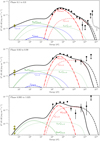 |
Fig. 3. Phase ranges off-periastron (upper), pre-periastron (middle) and periastron (lower) SEDs. Black data points represent the points from our Fermi-LAT analysis (Sect. 2.4); olive points show data from NuSTAR (Hamaguchi et al. 2018). The black solid line shows the total emission from our model with absorption. The black dashed line shows the same without absorption. Blue lines show the emission from electrons, green lines indicate the contribution from secondary particles, and red lines from protons of η Car A (bold) and η Car B (thin). In the upper plot (phase 0.1–0.9) upper limits from H.E.S.S. were added in grey (Abramowski et al. 2012). |
At off-periastron we find that primary electrons (indicated with blue lines in Fig. 1) are required to explain the level of emission seen with NuSTAR. We fix the relative fraction of energy going into primary electrons above a MeV to that in protons above a GeV at all phases for the two stars to be 3%. Inverse Compton emission from electrons accelerated at the side of η Car B dominates at NuSTAR energies, even if the fraction of energy going into the electrons of η Car A is increased by one order of magnitude. Pion decay from proton interaction on the side of η Car A is, in all phase ranges, the main contributor to the low-energy Fermi-LAT component of the SED, whereas at higher energy, protons from η Car B can account for the observed flux and spectrum. At periastron we switched off the injection of electrons. The level of the NuSTAR emission is consistent with the emission from secondary particles and no primary electrons are required in our model to match the data. This might be a hint for the consideration mentioned in Sect. 3 that at periastron the nature of the shock is changed, such that electron acceleration is quenched.
The spectral breaks at lower energies in the IC emission are associated with the transition between Coulomb and IC cooling (see Eq. (3)) and occur at different energies owing to the large range of different densities associated with the two shocks and the mixing region beyond the shock cap.
Absorption is important for energies above 100 GeV and therefore mainly affects the emission from η Car B. Stronger absorption occurs during periastron compared to the other phases owing to the small spatial extent of the emission region and the proximity to the two stars. However, this would change with the size of the emission region, which depends on the mixing length scale in the ballistic region.
The emission from protons of η Car B increases more towards periastron than for η Car A. The reason for this is the escape of accelerated protons at the side of η Car B, which do not contribute to the γ-ray emission. Towards periastron the density increases and more particles can interact.
Comparing the emission from electrons accelerated directly at the shocks (blue curves in Fig. 3), there are two effects which result in reduced radiation from the side of η Car A compared to η Car B (despite similar values of Pp and Pe/Pp, see Table 1). First, approximately four times less power is available in the wind at the shock on the side of η Car A; see O15. Additionally, the denser environment at the side of η Car A leads to much stronger Coulomb-Ionisation losses. Less power and more losses reduce the energy going into IC radiation.
5. Discussion and conclusions
Based on the new Fermi-LAT analysis, the basic physical arguments of Sect. 3, and the SED modelling of Sect. 4, several important conclusions regarding the non-thermal processes in η Car can be reached. We consider each of these in turn.
5.1. Pion-decay origin of the GeV emission
The spectral shape of the emission seen with Fermi-LAT between 0.1 and 10 GeV, as shown in Fig. 1, strongly favours a pion decay origin. This conclusion is consistent with our previous arguments in O15, based on simple energetic considerations of a two-shock system. In our model, the emission at the lower end of the Fermi-LAT band is dominated by protons accelerated at the shock of η Car A; see Fig. 3. The maximum energy at the shock is limited by hadronic interactions in the dense wind. The lower densities associated with the shock on the side of η Car B allow for larger maximum energies, the latter being limited only by escape from the shock cap. These protons thus account for the high-energy tail of the Fermi-LAT measurements, where the γ-rays are produced primarily as the shocked plasma from η Car B, with entrained high-energy particles, mixes with the denser material from η Car A in the exhausts of the WCR. The detailed physics of the mixing affects not only the cooling of protons and resulting γ-ray emission, but also the cooling break of secondary pairs. We found that the simple mixing-length profile adopted in our model provides a reasonable match to the data, but a more sophisticated model may be necessary to capture specific features.
5.2. Leptonic emission
Whilst there is a consensus that emission above 10 GeV is produced in hadronic interactions, the origin of the emission between 0.1 GeV and 10 GeV is still under debate (e.g. O15; Reitberger et al. 2015; Balbo & Walter 2017; Hamaguchi et al. 2018). Hamaguchi et al. (2018) have argued that the emission observed at these energies might represent a smooth continuation of the hard spectrum emission seen at 10s of keV arising from the IC emission of a hard electron spectrum. This scenario is strongly disfavoured by the new low-energy Fermi-LAT data points. In principle, as the IC emission from the primary electrons of η Car B can account for the NuSTAR data, a significantly harder lepton population accelerated at η Car A could be contrived to match the low-energy end Fermi-LAT data. However, this would require an equilibrium spectrum that is harder than E2dN/dE ∝ E1/2, which is incompatible with standard DSA theory. It is also difficult to disregard the coincidence between the position of the low-energy roll-over at ≲300 MeV with the threshold energy for pion production.
In addition, the strong orbital variability observed with NuSTAR (Hamaguchi et al. 2018), in contrast with the modest variability in the γ-ray flux, is also difficult to reconcile with a single electron population producing the emission in both energy bands.
Finally we note that previous leptonic models relied on a similar fraction of shocked wind power being injected into both the leptonic and hadronic components (e.g. Farnier et al. 2011; Balbo & Walter 2017). This is in contrast with emission models of supernova remnants, which typically require of order 10% of the dissipated shock power being transferred to protons and a ratio of accelerated electrons to protons at a fixed energy ∼10−4 − 10−2 (e.g. Helder et al. 2010; Zirakashvili & Aharonian 2010). Our results, which now disfavour the leptonic models, are more in line with such predictions.
5.3. NuSTAR observations
The non-thermal component in the NuSTAR data (Hamaguchi et al. 2018) confirms the presence of primary electrons. As discussed in Sect. 3, the equilibrium electron spectrum in the system must include a break associated with the transition from dominant Coulomb ionisation to IC cooling. For η Car A, the break in the IC spectrum is at a few MeV, while for η Car B it can fall close to the NuSTAR band (see for example Hinton & Hofmann 2009 or directly from the IC breaks in Fig. 3). In any case, the IC spectrum is expected to soften between the NuSTAR and Fermi-LAT bands, which is consistent with the hard NuSTAR spectrum.
Far from periastron, the NuSTAR flux is compatible with IC emission originating almost exclusively from the primary electrons accelerated at the shock of η Car B. In this regard, the fractional power injected into electrons at η Car A is effectively unconstrained. The NuSTAR minimum around periastron agrees with the level of emission expected for secondary electrons. The reason for the absence of primary electrons during this phase is not yet certain and will require more detailed kinetic simulations. However, the persistence of the Fermi-LAT γ-ray flux (see Fig. 2) is a clear indication that both shocks at the edges of the WCR are continuously accelerating protons. The absence of measurable X-ray flux from primary electrons therefore is most probably a consequence of suppression of electron heating/scattering, which we interpret as being due to low Alfvén Mach number in the case of η Car A, and a runaway of the whistler phase speed near periastron in the case of η Car B (see Sect. 3). The only contribution at hard X-rays would then be the emission from secondary particles from hadronic interactions of the freshly accelerated protons. Continuous monitoring of the reduction and subsequent recovery, during and following the periastron passage, would provide a unique window into the physical processes taking place in this extreme environment.
5.4. Maximum particle energies and neutrino fluxes
As noted by Gupta & Razzaque (2017), neutrino emission from η Car is potentially detectable if high enough particle energies can be reached. Away from periastron the cut-off energy of the protons is constrained to about 400 GeV by Fermi-LAT data and H.E.S.S. limits (see Fig. 3). At periastron, the current experimental data only constrain the cut-off energy to be greater than ≈500 GeV. In the framework of our model, the cut-off proton energy is limited to ∼1 TeV. The SED of neutrino emission from interacting protons peaks at more than an order of magnitude lower energies and would be overwhelmed by the atmospheric neutrino flux (see e.g. Kappes et al. 2007). Even in the extreme case of ηacc = 1 (leading to an exponential cut-off above 12 TeV the resulting expected neutrino fluxes, being less than 2 × 10⁻¹¹ erg cm−2 s−1 above 1 TeV and less than 3.3 × 10⁻¹³ erg cm−2 s−1 above 10 TeV, make η Car an unlikely source for astrophysical neutrino detection.
5.5. H.E.S.S. observations
The maximum γ-ray energies around periastron are not constrained by observations so far. Existing and future H.E.S.S. detections of η Car will allow us to further constrain Emax. In our model, strong absorption occurs at periastron (see Fig. 3), which is caused by the close vicinity to the stars and the relatively small size of the emission region compared to apastron. A larger size of the ballistic region due to a larger mixing length would reduce the absorption effects and therefore a detection by H.E.S.S. would give information about the location and spatial extent of the emission region.
The physical conditions in the shocks within the η Car system are dramatically different from any other well-measured particle accelerating system. As such they represent an extremely promising laboratory to study the phenomenon of particle acceleration. The dense and luminous environments provide an interesting comparison with the relatively new class of γ-ray novae (Ackermann et al. 2014). This has been previously noted by Vurm & Metzger (2018), who also discuss the connections with WCRs. The strong evidence reported in this paper in support of the hadronic origin of the Fermi-LAT data for η Car motivates a deeper study into other binary colliding wind systems.
Of particular interest are the implications for these new measurements on one of the outstanding problems of high-energy astrophysics, namely DSA and the interplay of the accelerated particle population with its self-excited magnetic fields. The current supernova cosmic-ray origin paradigm for example makes many assumptions regarding the non-linear behaviour of field amplification, and its ultimate role in the energetic particle transport and acceleration. Testing these assumptions with numerical simulations in a self-consistent manner is currently not possible, making η Car a powerful laboratory. While there are many aspects of the environment of η Car that are quite unique, it is nevertheless remarkable that within each complete orbit of the system the shocks sample a broad range of the parameter space relevant to DSA in Galactic supernovae. In this paper, we have shown that magnetic-field geometry, non-linear shock acceleration and magnetic-field amplification, and other plasma-physics considerations are essential to match observations accurately. With future observations and improved statistics, more detailed predictions of the above-mentioned processes can be put to the test.
The Fermi ScienceTools are distributed by the Fermi Science Support Center (http://fermi.gsfc.nasa.gov/ssc).
In the past a cut on the rocking angle was also recommended, but is no longer deemed necessary.
Acknowledgments
We thank F. Conte for providing the calculations for the cascading of the energy from γγ-absorption and C. Duffy for cross-checks of Fermi-LAT analysis. BR gratefully acknowledges valuable discussions with J. Mackey, and also with D. Eichler and D. Burgess during the Multiscale Phenomena in Plasma Astrophysics workshop at the Kavli Institute for Theoretical Physics.
References
- Abdo, A. A., Ackermann, M., Ajello, M., et al. 2009, ApJS, 183, 46 [NASA ADS] [CrossRef] [Google Scholar]
- Abdo, A. A., Ackermann, M., Ajello, M., et al. 2010, ApJ, 723, 649 [NASA ADS] [CrossRef] [Google Scholar]
- Abramowski, A., Acero, F., Aharonian, F., et al. 2012, MNRAS, 424, 128 [NASA ADS] [CrossRef] [Google Scholar]
- Achterberg, A. 2004, in Accretion Discs, Jets and High Energy Phenomena in Astrophysics, eds. V. Beskin, G. Henri, F. Menard, G. Pelletier, & J. Dalibard, 78, 313 [NASA ADS] [Google Scholar]
- Ackermann, M., Ajello, M., Albert, A., et al. 2014, Science, 345, 554 [NASA ADS] [CrossRef] [Google Scholar]
- Aharonian, F. A., & Atoyan, A. M. 1981, Ap&SS, 79, 321 [NASA ADS] [Google Scholar]
- Balbo, M., & Walter, R. 2017, A&A, 603, A111 [NASA ADS] [CrossRef] [EDP Sciences] [Google Scholar]
- Bednarek, W., & Pabich, J. 2011, A&A, 530, A49 [NASA ADS] [CrossRef] [EDP Sciences] [Google Scholar]
- Bell, A. R. 2004, MNRAS, 353, 550 [Google Scholar]
- Bosch-Ramon, V., & Khangulyan, D. 2009, Int. J. Mod. Phys. D, 18, 347 [NASA ADS] [CrossRef] [Google Scholar]
- Canto, J., Raga, A. C., & Wilkin, F. P. 1996, ApJ, 469, 729 [NASA ADS] [CrossRef] [Google Scholar]
- Castor, J. I., Abbott, D. C., & Klein, R. I. 1975, ApJ, 195, 157 [NASA ADS] [CrossRef] [Google Scholar]
- Corcoran, M. F. 2005, AJ, 129, 2018 [NASA ADS] [CrossRef] [Google Scholar]
- Corcoran, M. F., & Hamaguchi, K. 2007, Rev. Mex. Astron. Astrofis. Conf. Ser., 30, 29 [NASA ADS] [Google Scholar]
- Corcoran, M. F., Hamaguchi, K., Liburd, J. K., et al. 2015, ArXiv e-prints [arXiv:1507.07961] [Google Scholar]
- Corcoran, M. F., Liburd, J., Morris, D., et al. 2017, ApJ, 838, 45 [NASA ADS] [CrossRef] [Google Scholar]
- Dame, T. M., Hartmann, D., & Thaddeus, P. 2001, ApJ, 547, 792 [NASA ADS] [CrossRef] [Google Scholar]
- Damineli, A., Hillier, D. J., Corcoran, M. F., et al. 2008, MNRAS, 384, 1649 [NASA ADS] [CrossRef] [Google Scholar]
- Davidson, K., & Humphreys, R. M. 1997, ARA&A, 35, 1 [NASA ADS] [CrossRef] [Google Scholar]
- Dubus, G. 2006, A&A, 451, 9 [NASA ADS] [CrossRef] [EDP Sciences] [Google Scholar]
- Edmiston, J. P., & Kennel, C. F. 1986, J. Geophys. Res., 91, 1361 [NASA ADS] [CrossRef] [Google Scholar]
- Eichler, D., & Usov, V. 1993, ApJ, 402, 271 [NASA ADS] [CrossRef] [Google Scholar]
- Farnier, C., Walter, R., & Leyder, J. 2011, A&A, 526, A57 [NASA ADS] [CrossRef] [EDP Sciences] [Google Scholar]
- Fermi-LAT Collaboration 2020, ApJS, 247, 33 [NASA ADS] [CrossRef] [Google Scholar]
- Gould, R. J. 1975, ApJ, 196, 689 [NASA ADS] [CrossRef] [Google Scholar]
- Gupta, N., & Razzaque, S. 2017, Phys. Rev. D, 96, 123017 [NASA ADS] [CrossRef] [Google Scholar]
- Hamaguchi, K., Corcoran, M. F., Gull, T., et al. 2007, ApJ, 663, 522 [NASA ADS] [CrossRef] [Google Scholar]
- Hamaguchi, K., Corcoran, M. F., Russell, C. M. P., et al. 2014, ApJ, 784, 125 [NASA ADS] [CrossRef] [Google Scholar]
- Hamaguchi, K., Corcoran, M. F., Pittard, J. M., et al. 2018, Nat. Astron., 2, 731 [NASA ADS] [CrossRef] [Google Scholar]
- Helder, E. A., Kosenko, D., & Vink, J. 2010, ApJ, 719, L140 [NASA ADS] [CrossRef] [Google Scholar]
- Hillas, A. M. 1984, ARA&A, 22, 425 [NASA ADS] [CrossRef] [Google Scholar]
- Hillier, D. J., Davidson, K., Ishibashi, K., & Gull, T. 2001, ApJ, 553, 837 [NASA ADS] [CrossRef] [Google Scholar]
- Hinton, J. A., & Hofmann, W. 2009, ARA&A, 47, 523 [NASA ADS] [CrossRef] [Google Scholar]
- Iping, R. C., Sonneborn, G., Gull, T. R., Massa, D. L., & Hillier, D. J. 2005, ApJ, 633, L37 [NASA ADS] [CrossRef] [Google Scholar]
- Jean, P., Cheung, C. C., Ojha, R., van Zyl, P., & Angioni, R. 2018, ATel, 11546 [Google Scholar]
- Kappes, A., Hinton, J., Stegmann, C., & Aharonian, F. A. 2007, ApJ, 656, 870 [NASA ADS] [CrossRef] [Google Scholar]
- Leyder, J.-C., Walter, R., & Rauw, G. 2008, A&A, 477, L29 [Google Scholar]
- Mehner, A., Davidson, K., Humphreys, R. M., et al. 2015, A&A, 578, A122 [NASA ADS] [CrossRef] [EDP Sciences] [Google Scholar]
- Ohm, S., Zabalza, V., Hinton, J. A., & Parkin, E. R. 2015, MNRAS, 449, L132 (O15) [NASA ADS] [CrossRef] [Google Scholar]
- Parkin, E. R., Pittard, J. M., Corcoran, M. F., Hamaguchi, K., & Stevens, I. R. 2009, MNRAS, 394, 1758 [NASA ADS] [CrossRef] [Google Scholar]
- Parkin, E. R., Pittard, J. M., Corcoran, M. F., & Hamaguchi, K. 2011, ApJ, 726, 105 [NASA ADS] [CrossRef] [Google Scholar]
- Pittard, J. M., & Dawson, B. 2018, MNRAS, 477, 5640 [NASA ADS] [CrossRef] [Google Scholar]
- Rebolledo, D., Burton, M., Green, A., et al. 2015, MNRAS, 456, 2406 [Google Scholar]
- Reitberger, K., Reimer, A., Reimer, O., & Takahashi, H. 2015, A&A, 577, A100 [NASA ADS] [CrossRef] [EDP Sciences] [Google Scholar]
- Schlickeiser, R. 2002, Cosmic Ray Astrophysics (Berlin: Springer) [CrossRef] [Google Scholar]
- Tademaru, E. 1969, ApJ, 158, 959 [NASA ADS] [CrossRef] [Google Scholar]
- Tavani, M., Sabatini, S., Pian, E., et al. 2009, ApJ, 698, L142 [Google Scholar]
- Vurm, I., & Metzger, B. D. 2018, ApJ, 852, 62 [NASA ADS] [CrossRef] [Google Scholar]
- Walder, R., Folini, D., & Meynet, G. 2012, Space Sci. Rev., 166, 145 [NASA ADS] [CrossRef] [Google Scholar]
- Williams, P. M., Dougherty, S. M., Davis, R. J., et al. 1997, MNRAS, 289, 10 [NASA ADS] [Google Scholar]
- Wood, M., Caputo, R., Charles, E., et al. 2017, Proc. Int. Cosmic Ray Conf., 301, 824 [NASA ADS] [CrossRef] [Google Scholar]
- Zabalza, V. 2015, Proc. Int. Cosmic Ray Conf., 34, 922 [Google Scholar]
- Zirakashvili, V. N., & Aharonian, F. A. 2010, ApJ, 708, 965 [NASA ADS] [CrossRef] [Google Scholar]
Appendix A: Further Fermi-LAT analysis details
A.1. Data selection and model parameters
The full set of parameters used in the Fermi-LAT data selection and those used to construct a model of the region are listed in Table A.1; an explanation of the parameters is provided in the Fermi ScienceTools3 and FermiPy documentation (Wood et al. 2017).
Fermi-LAT data selection and model parameters used in this analysis.
A.2. Model residuals
Figure A.1 (upper) shows a residual TS map for a 4° by 4° region centred on η Car produced as a verification step post-likelihood fit as part of the analysis chain for a model based on only the 4FGL catalogue, diffuse Galactic template, and isotropic background component. Each point in the map shows the significance that would be attributed to an additional point source at that position. The position of η Car is denoted by a hollow white triangle. The two closest 4FGL catalogue sources are indicated by white crosses. It is clear that significant residual emission remains when following this standard approach. Overlaid are contours from a template generated from the CO measurements in Dame et al. (2001), which align well with the excess emission. Figure A.1 (lower) shows an equivalent TS map generated following a likelihood fit using a model including this additional diffuse component, indicating the improvement described in Sect. 2.2.
A.3. Systematic uncertainties
Systematic uncertainties were estimated for the SED generated from the total Fermi-LAT data set by varying analysis parameters and re-running the entire chain. The following parameters were varied:
– Energy range: Minimum energies between 60 and 120 MeV and maximum energies of 300 and 500 GeV were investigated.
– Region of interest: The ROI was varied between 5°, 10°, 15°, and 20°.
– Starting value for the CO template: The starting flux of the CO template was varied over an order of magnitude.
– Free parameters: Fits were run with model parameters allowed to vary under a number of conditions. Source normalisation was allowed to vary for sources within 3° and 5° of η Car with a TS > 10, 100, 1000. Shape parameters were also allowed to vary within the same distance of η Car with an additional selection of TS > 100, 1000, 10 000.
– SED energy binning: The SED energy binning was varied between 12 and 3 bins per decade.
The above variations resulted in hundreds of SEDs. At each point in each SED the fractional error from an interpolated mean SED was determined. The resulting distribution of fractional error as a function of energy was then fitted with a simple cubic polynomial. This function was then used to compute a smooth band around the SED points presented in Fig. 1 (grey area).
A.4. Orbital phase SED analysis
In Sect. 2.4 we describe phase-resolved SED analysis and in Sect. 4 the results are presented for a combined analysis of the Fermi-LAT data from both orbital periods in Fig. 3. Figure A.2 shows the sames results (grey solid lines) together with the data points obtained from independently analysing each orbital period. The first orbital period (periastron passage 2009) is shown by the blue data points and the second (periastron passage 2014) by the black data points.
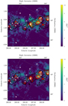 |
Fig. A.1. Residual TS maps, with default 4FGL catalogue sources included (upper) and with the CO template is included in the model (lower). The position of η Car is denoted by a hollow white triangle. The two closest 4FGL catalogue sources are indicated by white crosses. Overlaid are contours from a template generated from the CO measurements in Dame et al. (2001). |
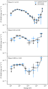 |
Fig. A.2. Fermi-LAT analysis SEDs for the same phase ranges presented in Fig. 3. The results from a combined analysis of both orbital periods is given by the solid grey lines. Results from an independent analysis of each orbital passage are shown by the data points (blue: periastron passage 2009, black: periastron passage 2014). |
All Tables
Adopted model parameters associated with the two stars in the η Car system and their associated wind shocks.
All Figures
|
Fig. 1. Spectral energy distribution resulting from Fermi-LAT analysis of η Car over the full data set (black points) together with a systematic error band (grey area). A fit to the data points below 200 GeV using the Naima package (Zabalza 2015) is shown by the black curve under the assumption that the γ-ray emission arises from proton-proton interactions with an exponential cutoff power-law distribution for the protons. Data points from a previous Fermi-LAT analysis (Reitberger et al. 2015) are shown in blue for comparison. |
| In the text | |
|
Fig. 2. Upper panel: Fermi-LAT temporal analysis of η Car from 300 MeV to 10 GeV from orbital phase 0.8 to 1.2 in 0.03 phase bins. Data corresponding to the first orbital period observed by the Fermi-LAT (with periastron in 2009) are shown in blue, and those corresponding to the second orbital period (with periastron in 2014) in black. Vertical grey shaded areas indicate the phase ranges used in the spectral analysis presented in Sect. 2.4 around periastron, pre-periastron, and off-periastron. The points from Balbo & Walter (2017) are shown as hollow grey circles. The vertical black dashed line indicates periastron. Middle panel: NuSTAR points for the 2014 periastron passage from Hamaguchi et al. (2018). Lower panel: RXTE and Swift data for the last four periastron passages. |
| In the text | |
|
Fig. 3. Phase ranges off-periastron (upper), pre-periastron (middle) and periastron (lower) SEDs. Black data points represent the points from our Fermi-LAT analysis (Sect. 2.4); olive points show data from NuSTAR (Hamaguchi et al. 2018). The black solid line shows the total emission from our model with absorption. The black dashed line shows the same without absorption. Blue lines show the emission from electrons, green lines indicate the contribution from secondary particles, and red lines from protons of η Car A (bold) and η Car B (thin). In the upper plot (phase 0.1–0.9) upper limits from H.E.S.S. were added in grey (Abramowski et al. 2012). |
| In the text | |
|
Fig. A.1. Residual TS maps, with default 4FGL catalogue sources included (upper) and with the CO template is included in the model (lower). The position of η Car is denoted by a hollow white triangle. The two closest 4FGL catalogue sources are indicated by white crosses. Overlaid are contours from a template generated from the CO measurements in Dame et al. (2001). |
| In the text | |
|
Fig. A.2. Fermi-LAT analysis SEDs for the same phase ranges presented in Fig. 3. The results from a combined analysis of both orbital periods is given by the solid grey lines. Results from an independent analysis of each orbital passage are shown by the data points (blue: periastron passage 2009, black: periastron passage 2014). |
| In the text | |
Current usage metrics show cumulative count of Article Views (full-text article views including HTML views, PDF and ePub downloads, according to the available data) and Abstracts Views on Vision4Press platform.
Data correspond to usage on the plateform after 2015. The current usage metrics is available 48-96 hours after online publication and is updated daily on week days.
Initial download of the metrics may take a while.