| Issue |
A&A
Volume 679, November 2023
|
|
|---|---|---|
| Article Number | A148 | |
| Number of page(s) | 19 | |
| Section | Planets and planetary systems | |
| DOI | https://doi.org/10.1051/0004-6361/202346394 | |
| Published online | 30 November 2023 | |
Compositional properties of planet-crossing asteroids from astronomical surveys★
1
Université Côte d’Azur, Observatoire de la Côte d’Azur, CNRS,
Laboratoire Lagrange, France
e-mail: This email address is being protected from spambots. You need JavaScript enabled to view it.
2
V. N. Karazin Kharkiv National University,
4 Svobody Sq.,
Kharkiv
61022, Ukraine
3
European Southern Observatory (ESO),
Alonso de Cordova 3107,
1900
Casilla Vitacura, Santiago, Chile
4
Department of Earth, Atmospheric and Planetary Sciences, MIT,
77 Massachusetts Avenue,
Cambridge, MA
02139, USA
5
Astronomical Institute, Academy of Sciences of the Czech Republic,
25165
Ondřejov, Czech Republic
6
INAF – Osservatorio Astronomico di Roma,
Via Frascati 33,
00078
Monte Porzio Catone, Italy
7
Department of Earth, Atmospheric, and Planetary Sciences, Massachusetts Institute of Technology,
77 Massachusetts Avenue,
Cambridge, MA
02139, USA
8
INAF – Osservatorio Astronomico di Roma,
Monte Porzio Catone (RM), Italy
9
INAF – Department of Physics and Astronomy, University of Padova,
Vicolo dell’Osservatorio 3,
35122
Padova, Italy
10
Agenzia Spaziale Italiana (ASI),
Via del Politecnico,
00133
Roma, Italy
Received:
13
March
2023
Accepted:
18
July
2023
Abstract
Context. The study of planet-crossing asteroids is of both practical and fundamental importance. As they are closer than asteroids in the Main Belt, we have access to a smaller size range, and this population frequently impacts planetary surfaces and can pose a threat to life.
Aims. We aim to characterize the compositions of a large corpus of planet-crossing asteroids and to study how these compositions are related to orbital and physical parameters.
Methods. We gathered publicly available visible colors of near-Earth objects (NEOs) from the Sloan Digital Sky Survey (SDSS) and SkyMapper surveys. We also computed SDSS-compatible colors from reflectance spectra of the Gaia mission and a compilation of ground-based observations. We determined the taxonomy of each NEO from its colors and studied the distribution of the taxonomic classes and spectral slope against the orbital parameters and diameter.
Results. We provide updated photometry for 470 NEOs from the SDSS, and taxonomic classification of 7401 NEOs. We classify 42 NEOs that are mission-accessible, including six of the seven flyby candidates of the ESA Hera mission. We confirm the perihelion dependence of spectral slope among S-type NEOs, likely related to a rejuvenation mechanism linked with thermal fatigue. We also confirm the clustering of A-type NEOs around 1.5–2 AU, and predict the taxonomic distribution of small asteroids in the NEO source regions in the Main Belt.
Key words: minor planets, asteroids: general / methods: data analysis / surveys / techniques: photometric
The catalog is available at the CDS via anonymous ftp to cdsarc.cds.unistra.fr (130.79.128.5) or via https://cdsarc.cds.unistra.fr/viz-bin/cat/J/A+A/679/A148
The NEOROCKS team: E. Dotto, M. Banaszkiewicz, S. Banchi, M.A. Barucci, F. Bernardi, M. Birlan, A. Cellino, J. De Leon, M. Lazzarin, E. Mazzotta Epifani, A. Mediavilla, J. Nomen Torres, E. Perozzi, C. Snodgrass, C. Teodorescu, S. Anghel, A. Bertolucci, F. Calderini, F. Colas, A. Del Vigna, A. Dell’Oro, A. Di Cecco, L. Dimare, P. Fatka, S. Fornasier, E. Frattin, P. Frosini, M. Fulchignoni, R. Gabryszewski, M. Giardino, A. Giunta, T. Hromakina, J. Huntingford, S. Ieva, J.P. Kotlarz, M. Popescu, J. Licandro, H. Medeiros, F. Merlin, F. Pinna, G. Polenta, A. Rozek, P. Scheirich, A. Sonka, G.B. Valsecchi, P. Wajer, A. Zinzi.
© The Authors 2023
 Open Access article, published by EDP Sciences, under the terms of the Creative Commons Attribution License (https://creativecommons.org/licenses/by/4.0), which permits unrestricted use, distribution, and reproduction in any medium, provided the original work is properly cited.
This article is published in open access under the Subscribe to Open model. This email address is being protected from spambots. You need JavaScript enabled to view it. to support open access publication.
1 Introduction
Asteroids are the remnants of the building blocks that accreted to form the terrestrial planets and the core of the giant planets in the early Solar System 4.6 Gyr ago. Asteroids are also the origin of the meteorites that fell on the planets, including the Earth. These meteorites represent the only possibility to study in detail the composition of asteroids in the laboratory (e.g., Consolmagno et al. 2008; Cloutis et al. 2015), with the exception of the tiny samples of rock, provided by return-sample missions: JAXA Hayabusa (Yurimoto et al. 2011) and Hayabusa-2 (Tachibana et al. 2022), as well as the soon due NASA OSIRIS-REx (Lauretta et al. 2017).
In contrast to targeted sample collection, we cannot choose the origin of meteorites striking the Earth. Identifying their source regions is therefore crucial to determining the physical conditions and abundances in elements that reigned in the proto-planetary nebula around the young Sun (McSween et al. 2006). From the analysis of a bolide trajectory, it is possible to reconstruct a meteorite’s heliocentric orbit (Gounelle et al. 2006), although such determinations have been limited to only a few meteorites (Granvik & Brown 2018).
Among the different dynamical classes of asteroids, the near-Earth and Mars-crosser asteroids (NEAs and MCs), whose orbits cross that of the telluric planets, form a transient population. Their typical lifetime is of only a few million years before they are ejected from the Solar System, fall into the Sun, or impact a planet (Gladman et al. 1997). We refer here to near-Earth objects (NEOs) in a liberal sense, encompassing both asteroid-like and comet-like objects whose orbits cross that of a terrestrial planet (hence including NEAs, MCs, and some Hungarias).
These populations are of both scientific and pragmatic interest. As they are closer to the Earth than the asteroid belt, we have access to smaller objects from ground-based telescopes. Their orbital proximity implies a much smaller impulsion to reach them with a spacecraft and make them favorable targets for space exploration (Abell et al. 2012). On the other hand, these objects could potentially pose a threat, and studying their properties is a key aspect in planning risk mitigation (Drube et al. 2015), of which the National Aeronautics and Space Administration (NASA) Demonstration for Autonomous Rendezvous Technology (DART) and European Space Agency (ESA) Hera missions are lively demonstrators (Rivkin et al. 2021; Michel et al. 2022).
We focus here on the compositional properties of a large corpus of NEOs as part of the NEOROCKS project (Dotto et al. 2021), whose goal is the characterization of the NEO population. The article is organized as follows. In Sect. 2, we present the data we have collected and the way in which we are building a large catalog of NEOs with visible colors (including a refinement of the photometry of the NEOs present in the SDSS catalog, Appendix B). We then present in Sect. 3 the way in which we determine the taxonomic class of each NEO. We focus on the taxonomy of the potential targets for space missions in Sect. 4, and finally, we discuss the distribution of taxonomic classes, the effect of space weathering and planetary encounters, and NEO source regions in Sect. 5.
2 Data sources
In this section, we describe the data sets we collect, how they compare in terms of precision, and the way in which we merge them into a single catalog of colors. The entire process is summarized in Fig. 1.
2.1 Collecting data sets
We gathered the colors of NEOs from four recently published sources: the Sloan Digital Sky Survey (SDSS; Sergeyev & Carry 2021), the SkyMapper Southern Survey (SMSS; Sergeyev et al. 2022), the Gaia DR3 visible spectra (Gaia; Gaia Collaboration 2023b), and a compilation of ground-based spectra (Classy; Mahlke et al. 2022). For the last two sources, we converted the reflectance to colors in order to obtain the largest possible homogeneous data set (Appendix A).
Each SDSS observation sequence contains quasi-simultaneous measurements in five filters (u, g, r, i, z), providing colors of all combinations. There is a constant time difference between two exposures in consecutive filters, equal to 57 s. The largest time difference between two exposures occurs for the g and r filters, and is approximately 230 s. The initial SDSS catalog contains 11142 individual multi-filter observations of 5425 unique NEOs. For each NEO, we computed the weighted mean of each color from multiple measurements. Owing to potential biases on the SDSS photometry for fast-moving NEOs (Solano et al. 2014; Carry et al. 2016), we remeasured 470 NEO colors on SDSS frames (see Appendix B).
The SkyMapper includes several observing strategies. A shallow six-filter sequence with exposure times between 5 s and 40 s, a deep ten-image sequence of uvgruvizuv with 100 s exposures, and pairs of deep exposures in (g,r) and (i,z). This observing strategy, in conjunction with the enhanced sensitivity in g and r, implies a predominance of g – r colors in the results, but almost always leads to the measurement of at least one photometric color obtained within ≲ 2 min (see Sergeyev et al. 2022, for more details). The initial SkyMapper catalog contains 12 001 individual observations of 3149 unique NEOs. We computed the asteroid color indexes by limiting the observation time between two filters to 20 min and weighted the mean color of multiple asteroid measurements whenever possible. Through this method, we retrieved 9212 colors of 2081 individual NEOs. The SkyMapper filters are slightly different from those of SDSS. We thus converted the SkyMapper colors into SDSS colors using color-transformation coefficients that were computed from a wide range of stellar classes (Sergeyev et al. 2022).
Gaia DR3 (Gaia Collaboration 2016, 2023a) contains 60 518 low-resolution reflectance spectra of asteroids (Gaia Collaboration 2023b). Among these, 838 are NEOs, of which 199 have not been recorded in other catalogs. These optical spectra range from 374 to 1034 nm, meaning that they almost fully overlap with SDSS g to z filters (see Fig. A.1). We thus converted the Gaia reflectance spectra to SDSS colors to homogenize the data set. We detail the procedure in Appendix A.
The Gaia DR3 represents the largest catalog of asteroid reflectance spectra. However, the spectra of NEOs have regularly been acquired with ground-based facilities for decades, often over a larger wavelength range and with a higher spectral resolution (e.g., NEOSHIELD2, MITHNEOS, and MANOS surveys, see Perna et al. 2018; Binzel et al. 2019; Devogèle et al. 2019). Therefore, we used the preprocessed and resampled ground-based spectra from Mahlke et al. (2022), which comprises 4548 spectra of 3157 unique asteroids. We extracted 1072 spectra of 846 unique NEOs and converted them to SDSS colors with the same procedure as for the Gaia data (Appendix A).
2.2 Comparing data sets
Before merging the four catalogs of colors, we checked for systematic differences in colors and uncertainties among the four data sets. To do this, we did not restrict the comparison to NEOs, but used all of the available asteroid colors from the entire four data sets: 400 894 for SDSS, 139 220 for SMSS, 60 518 for Gaia, and 3157 for ground-based (Classy).
We cross-matched the asteroid colors from the other sources to the SDSS, which contains the largest number of asteroids and is used as a reference here. We found 67 921, 28 948, and 1951 asteroids in common for the SMSS, Gaia, and Classy catalogs, respectively. We then computed the color difference between the SDSS and the other catalogs. The distribution of these differences were normal for all pairs of filters and catalogs, with mean values close to zero (Fig. 2). The spread (standard deviation) of these differences reflects a combination of several effects: the measurement uncertainties of each catalog (either magnitudes or spectra), the potential effect of asteroid rotation (due to the non-simultaneous acquisition of asteroid images in different filters; see, e.g., Carry 2018) and observations at different phase angles (Sanchez et al. 2012; Gaia Collaboration 2023b; Cellino et al. 2020).
The detailed results of this comparison are presented in Table 1. There are small systematic offsets between catalogs on average, much smaller than their standard deviation but larger than the standard error ( , where n is the number of observations). For instance, SMSS matches SDSS with an average g-r color difference of 0.033 mags and a standard deviation of 0.106 magnitude. This was determined using 44 005 shared g-r color measurements that had an error of less than 0.1 magnitude. Although the systematic offset is three times smaller than the standard deviation, the standard error is approximately 0.0005. Therefore, these systematic biases were corrected by adding the precomputed offsets for each color before merging the data sets.
As visible in Fig. 2, the width of the color difference distributions is largest between SDSS and SMSS, because both catalogs have the largest color uncertainties. Once the color difference between the catalogs is corrected, the standard deviation can be independently computed as
 (1)
(1)
We present a detailed comparison of the color differences and uncertainties in Appendix C. Based on this analysis, we note that some uncertainties are either over- or under-estimated (e.g., Gaia and SMSS, respectively), and we applied multiplicatively correcting factors to select the best color value between identical asteroid color measurements in the catalogs (see Table C.1).
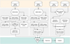 |
Fig. 1 Schematic view of the extraction, convertion, and merging of NEOs from SDSS, SMSS, Gaia, and Classy catalogs. |
2.3 Merging data sets
We merged the four data sets based on asteroid designation (we used the rocks1 interface to the name resolver of SsODNet2, see Berthier et al. 2023). Each catalog contains NEOs that have not been measured in the others. The most prolific source is the SDSS, which contains 4398 unique NEOs, followed by SkyMapper, with 964 unique NEOs. The Classy and Gaia catalogs contain 507 and 199 unique NEOs, respectively.
For NEOs present in more than one catalog, the color with the smallest uncertainty is selected. This results in a catalog of 7401 NEOs (i.e., NEAs and MCs) with at least one color measurement, which we call NEOROCKS. We collected the ancilllary parameters of each asteroid in our sample with SsODNet, including orbital elements and albedo, for instance. The description of the catalog is presented in Appendix E.
We present in Fig. 3 the orbital distribution of the NEOROCKS sample and detail in Table 2 the dynamical classes, including 2277 NEOs (Aten, Amor, Apollo, and Atira) and 5124 MCs. We also included the Hungarians that, owing to their eccentricity, have a perihelion within the orbit of Mars in the MC sample.
The absolute magnitudes in the NEOROCKS catalog extracted from the virtual observatory Solar System open database network (SsODNet; Berthier et al. 2023) show a bimodal distribution (Fig. 4), resulting from the typical larger distance of MCs compared with NEAs. The average absolute magnitude of the NEAs is 19.2 ± 2.0, while it is 17.8 ± 1.3 for MCs. Assuming an albedo of 0.24 for all NEOs results in an average diameter of  km for NEAs and
  km for MCs, covering a complessive range from ≈ 10 km down to 50 m. We chose this albedo as it is the mean albedo of S-type asteroids (Mahlke et al. 2022), the most represented taxonomic class among NEOs (Sect. 5 and, e.g., Binzel et al. 2019).
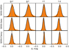 |
Fig. 2 Distribution of color differences between the SMSS, Gaia, and Classy with respect to the SDSS data set, using asteroids commonly found in these data sets. The distribution was fitted with a Gaussian curve, represented by the black line. The central gray vertical line denotes the zero offset. |
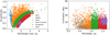 |
Fig. 3 Distribution of the orbital elements of the NEOs, color-coded by dynamic class. |
Mean and standard deviation of the color difference between SDSS and the other samples.
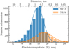 |
Fig. 4 Distribution of absolute magnitude of MCs (blue) and NEAs (orange). The diameter scale is a guideline, computed with an average albedo of 0.24. |
Distribution of NEOs among dynamic classes.
3 Taxonomy
Taxonomy is a convenient way to summarize observations into a simpler set of labels that describe categories of objects that share the same properties. Asteroid taxonomy is based on the spectral signatures of the light reflected by the surface (e.g., Belskaya et al. 2015; Reddy et al. 2015). Widely used asteroid taxonomy schemes include those of Tholen (1984), using visible colors and albedo, and DeMeo et al. (2009), using visible and near-infrared spectrum (itself an extension of Bus & Binzel 2002, based on the visible spectrum). These have recently been unified into a taxonomy using both visible and near-infrared spectra and albedos (Mahlke et al. 2022).
3.1 Classification of multi-color NEOs
We used the same approach as earlier works on photometry, deriving consistent classification with spectroscopy (e.g., DeMeo & Carry 2013; Popescu et al. 2018a; Sergeyev & Carry 2021). We converted reference spectra into colors (Appendix A) and used them to define the taxonomic class in the photometry space. To determine the taxonomic class of each asteroid, we employed the probabilistic approach of Sergeyev et al. (2022), which involves computing the intersection between the volume occupied by the color (with uncertainty) of an object and the regions of each taxonomic class. We updated the regions to match the recent taxonomy by Mahlke et al. (2022) instead of using the templates from Bus-DeMeo (DeMeo et al. 2009) and computed the probability for each asteroid belonging to each of the ten broad taxonomy complexes: A, B, C, D, K, L, Q, S, V, and X.
The final taxonomy for each asteroid was selected based on the most probable taxonomic complex. We also provided the second-highest probability taxonomic complex. Asteroids with a likelihood of less than 10% fitting into any taxonomy complex were labeled as U (unclassified; Appendix E).
We present in Fig. 5 the color-color distribution of 2341 NEOs for which taxonomy is predicted with a probability higher than 20%. This constraint was selected to avoid the visual overloading of the figure. The distribution follows the reported color distribution of asteroids in the SDSS filter system (Nesvorný et al. 2005; Parker et al. 2008; Carry et al. 2016). We also present a comparison of pseudo-reflectance spectra based on the photometry of our sample with the template spectra of the taxonomic class from Mahlke et al. (2022) in Fig. 6. The correspondence of the SDSS median spectra with the template spectra confirms the chosen taxonomy boundaries. The method provides a reliable way to determine the taxonomic classification of NEOs using photometry data. With the increasing number of NEOs discovered every year, it is becoming increasingly important to be able to classify these objects accurately and efficiently. Spectroscopy is the most accurate method for determining asteroid taxonomy, but it is time-consuming and requires a significant amount of telescope time. On the other hand, photometry data can be obtained much more efficiently, making it a more practical choice for large-scale surveys.
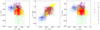 |
Fig. 5 Color-color distribution NEOs with a taxonomy probability above 0.2, color-coded by taxonomic classes. |
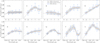 |
Fig. 6 Pseudo-reflectance spectra of asteroids based on their g-r, g-i, and i-z colors. The distribution of values for each band is represented by whiskers (95% extrema, and the 25, 50, and 75% quartiles). For each class, we also represent the associated template spectra of the Mahlke et al. (2022) taxonomy. |
3.2 Classification based on a single color
Many observations in the present data set have a significantly better signal-to-noise ratio in the g and r filters. Furthermore, some of the asteroids from the SMSS sample only have g-r color. Thus we also classified asteroids from this single color. We utilized the g-r color of one million asteroid observations from Sergeyev & Carry (2021) to build a reference distribution. We fitted this distribution with two normal distributions, corresponding to two wide complexes (carbonaceous, C1, and silicates, S1). We used these two distributions to compute the probability that a NEO belongs to each wide complex, based on its g-r color. Whenever the difference between the probabilities was smaller than 20 percent, we marked these asteroids as unclassified. We present the g-r color distribution of NEOs in Fig. 7. It is of course a cruder classification than the classification based on three colors. However, it allows for discrimination between “red” (S, A, V, L, and D) and “blue” objects (C and B) in a manner similar to Erasmus et al. (2020). A significant number of the unclassified asteroids belong to the X complex, while the remainder are of the D- and K-asteroid types (Fig. 8). Although a taxonomy based on a single color may appear limited, we present in Fig. 8 the confusion matrix between the one- and three-color classes. The C1 and S1 classes accurately separate asteroids belonging to the C complex from those displaying an absorption band of around 1 micron (which are redder: K types, L types, and S complex).
As a final step, we merged the taxonomy obtained with three colors (g-r, g-i, and i-z) and that with a single color only (g-r). The former is preferred over the latter (Appendix E). If neither approach could classify an asteroid, we set the classification method to “none.”
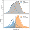 |
Fig. 7 Distribution of g-r colors in SDSS asteroids and taxonomic categorization of NEOs. Top: Color distribution of one million asteroids obtained from the SDSS (Sergeyev & Carry 2021) data set modeled by fitting a mixture of two Gaussians (represented by the black line). The two main taxonomic classes, silicate (depicted in orange) and carbonaceous (depicted in blue), were represented by the model. Bottom: Distribution of g-r colors and the taxonomy of NEOs analyzed using the two-component mixture model of the two primary classes in the SDSS data set (shown by lines). The carbonaceous and silicate taxonomy complexes are represented by blue and orange, respectively. Unclassified asteroids, where the probability of belonging to each complex is comparable, are represented in gray. |
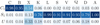 |
Fig. 8 Confusion matrix illustrating the correlation between predicted single-color (g-r) taxonomy outcomes and the results of a three-color taxonomy (g-r, g-i, i-z). This matrix displays the fractions of true positives, false positives, true negatives, and false negatives. |
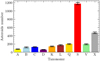 |
Fig. 9 NEO taxonomy distribution computed by (g-r, g-i, i-z) color indexes. |
3.3 Distribution of taxonomy and albedos
The prevalence of S types is striking (Fig. 9). It is notable that the distribution presented here is influenced by the selection function of the observations, which introduces a bias, mainly due to the fact that the surveys used here are magnitude limited, which will impact different taxonomic classes of different albedos (DeMeo & Carry 2013; Marsset et al. 2022). The albedo is an important characteristic related to the composition of asteroids (Tholen 1989; Mahlke et al. 2022). For instance, asteroids in the B, C, and D classes have low albedos (below 10%) while mafic-silicate-rich asteroids (e.g., A, Q, and S types) have albedos around 0.24. The main advantage of taking the albedo into account is the possibility to split the degenerate X complex into high albedo E-type asteroids (albedo above 0.30), moderate albedo M (metallic) asteroids, and the “dark” P asteroids (below 0.10).
We used SsODNet (Berthier et al. 2023) to retrieve the albedo of the NEOs in our data set for a consistency check. In Fig. 10 we compare the i-z and g-r colors of 898 NEOs that have estimated albedo values. There is an overall agreement between the range of albedos for the different taxonomic complexes, although outliers are visible. These outliers are a consequence of either misclassifications or biased albedos (Masiero et al. 2021), or both. Mismatches occur mainly in classes with highly different albedos but similar colors, such as D- and L-type asteroids (here, some D types have albedos around 0.2, more consistent with L types).
The albedo distribution of X types reveals that approximately 45% of them are actually P types. The fraction of M types is approximately 45% and the remaining 10% are high-albedo E-type asteroids (Usui et al. 2013). However, P-type asteroids are very similar to C-type asteroids in both color and albedo, and can therefore be misclassified.
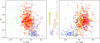 |
Fig. 10 Colors and albedo of NEOs. Taxonomy is marked by colored letters (same color-code as in Fig. 5). Vertical ranges between the panel indicate the one sigma range of albedo for each taxonomic class (Mahlke et al. 2022). |
3.4 Comparison with previous surveys
We compared the distribution of taxonomic classes of the present NEOROCKS sample with the three previous main spectral surveys of NEOs: MITHNEOS (Binzel et al. 2019), NEOSHIELD (Perna et al. 2018), and MANOS (Devogèle et al. 2019; see Fig. 11). The NEOROCKS sample overlaps almost completely with the NEOSHIELD-2 and MANOS catalogs because the Classy data include all available ground-based spectral observations. The overlap with MITHNEOS is limited to approximately half of this catalog, for which a majority of spectra only cover the near-infrared range. While differences are visible (and partly expected owing to the size dependence of taxonomic distribution; e.g., Devogèle et al. 2019), we note an overall agreement with the different data sets.
The confusion matrix presented in Fig. 12 indicates that there is a high level of agreement in the taxonomic classification of S-, V-, and X-type asteroids. However, some confusion is observed among the less common classes in the NEOs population, particularly K versus L and (A, L, Q) versus S. Additionally, a significant number of C-type asteroids were classified as part of the wide X asteroid complexes, which also include P-type asteroids that share similar photometry and albedo properties with C-type asteroids. This highlights both the strengths and limitations of using broadband colors as the basis for taxonomic classification.
4 Targets accessible to space missions
As opposed to other domains in astrophysics, the Solar System can almost be considered as a close neighborhood. Distances are small enough that we have sent space probes (some of which returned), providing ground-truths for Earth-based studies and leading to great discoveries, such as satellites of asteroids (Chapman et al. 1995; Belton et al. 1995), the asteroid-meteorite link (Fujiwara et al. 2006; Yurimoto et al. 2011), and cryo-volcanism (on Ceres, Küppers et al. 2014; Ruesch et al. 2016), for instance.
Since the 1990s, opportunities to encounter an asteroid during an interplanetary mission have been considered, and dynamical studies have been conducted to find candidates for potential flyby missions (e.g., Di Martino et al. 1990; Agostini et al. 2022). These candidates are often at the origin of characterization efforts to select the actual target of the flyby and prepare the spacecraft operations during the short encounter (e.g., Doressoundiram et al. 1999; Carry et al. 2010). As a result, there have been almost as many encounters (seven) during opportunity flybys3 as targeted encounters with asteroids4 (ten).
We searched in the present NEOROCKS data set for any candidate of upcoming space missions (e.g., NASA JANUS, JAXA Hayabusa-2 extension, Scheeres et al. 2020; Yano et al. 2022) and found many objects (Table 3) listed as flyby candidates for the ESA Hera mission (approximately one hundred, see Fitzsimmons et al. 2020).
A critical parameter in selecting a space mission target is the amount of energy required to reach it. This quantity is often expressed as the total change of velocity, Δυ. We collected Δυ computed and provided by L. Benner5 and for NEOs in our NEOROCKS catalog with a Δυ < 6.5 km, the typical Δυ required for a mission to Mars. We present in Table 4 the taxonomy of these 42 mission-accessible NEOs. We also provide an analysis of the spectrum for the flyby candidate (10278) Virkki in Appendix D.
Finally, we present the Gaia spectra for two candidates from the short list of seven candidates still considered for a flyby by Hera in Fig. 13. We also present the SDSS/SkyMapper colors of four other candidates.
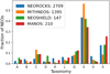 |
Fig. 11 Comparison of the distribution of taxonomic classes of the NEOROCKS sample computed from (g-r, g-i, i-z) color indexes with the MITHNEOS, NEOSHIELD, and MANOS spectral surveys. |
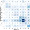 |
Fig. 12 Comparison of the NEOROCKS NEO taxonomy with the MITH-NEOS, MANOS, and NEOSHIELD-2 catalogs. |
Flyby candidates of the ESA Hera mission.
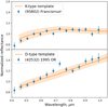 |
Fig. 13 Gaia reflectance spectra of asteroid (95 802) Francismuir and (42 532) 1995 OR, flyby candidates of the ESA Hera mission. The orange line shows pre-computed reflectance templates and their uncertainties (Mahlke et al. 2022) for P-type asteroids (top) and D-type asteroids (bottom). |
5 Discussion
We used the derived colors and taxonomic classes to address several topics. In Sect. 5.1, we discuss the space weathering for the NEOs in the S complex. We then present the distribution of A types in Sect. 5.2. We finally discuss the taxonomic distribution of small asteroids in the source regions of NEOs in Sect. 5.4.
5.1 Space weathering
The surface of atmosphereless bodies in the Solar System is aging from micro-meteorite impacts and ions of the solar wind, commonly referred to as space weathering (Chapman 2004). Space weathering changes the properties of the top-most surface layer (nanometer thick, Noguchi et al. 2011), as function of exposure (age and heliocentric distance) and composition. Thanks to laboratory experiments (e.g., Sasaki et al. 2001; Strazzulla et al. 2005; Brunetto et al. 2006), the effect of space weathering on mixtures of olivines and pyroxenes (such as A, S, and V types) is well understood (Brunetto et al. 2015): it reddens and darkens surfaces. Its effects on the reflectance of more primitive material linked with carbonaceous chondrites (such as B- and C-types) is less straightforward, with both blueing and reddening as possible outputs (Lantz et al. 2017, 2018).
In the case of S types, the effect is expected to be very fast, changing ordinary chondrite-like material (the Q types) into S types in less than a million years (Vernazza et al. 2009). The presence of Q types among asteroids implies that their surfaces are young. Considering the short timescale for space weathering (longer than the timescale to be injected from the Main Belt, Gladman et al. 1997), some rejuvenating mechanisms must be present (Marchi et al. 2012).
Q-type asteroids were originally found among NEOs only, so planetary encounters were proposed as a rejuvenation mechanism (Nesvorný et al. 2005, 2010; Binzel et al. 2010). However, this early observation was due to an observing bias: the fraction of Q increases toward smaller diameters, which are harder to observe at larger distances (Thomas et al. 2012; Carry et al. 2016). As space weathering is a continuous process (ultimately resulting in asteroids being classified into two groups: S and Q), the observed trend of shallower slopes among S/Q asteroids with smaller diameters explains this bias, and can be explained by a resurfacing due to landslides or failure linked with Yarkovsky-O’Keefe-Radzievskii-Paddack (YORP) spin-up (Graves et al. 2018).
Recently, Graves et al. (2019) tested another mechanism for rejuvenation among NEOs: a cracking mechanism due to thermal fatigue (Viles et al. 2010; Delbo et al. 2014). Based on almost 300 NEOs (from Lazzarin et al. 2004, 2005; Binzel et al. 2004), this model explains the overall behavior of spectral slope against perihelion, which was apparently misinterpreted as being linked to planetary encounters.
In the present section, we use the large NEOROCKS catalog to address the question of space weathering. Our sample contains 1175 S-type and 196 Q-type asteroids whose taxonomy is based on three colors with a probability higher than 0.2. We chose to use both the taxonomic types (i.e., the Q/S ratio) and the spectral slope as indicators of space weathering. The former highlights the fraction of very fresh surfaces in the sample, while the latter is more nuanced, with the weathering creating a continuous trend from blue to red surfaces.
We first studied the size dependence of space weathering of S-type asteroids. We present in Fig. 14 their spectral slope (computed over the g and i filters, expressed in % (μm)−1 consistently with reflectance spectroscopy) against their diameter. The diameter of the asteroids (D) was estimated using their known absolute magnitude (H) via the equation D = 1329 ·  (Harris & Lagerros 2002) and assuming an albedo of S-type asteroids pV = 0.24. The slope of S-type asteroids is constant for asteroids smaller than approximately 1–5 km, and increases for larger asteroids. This is consistent with the previous report by Binzel et al. (2004). Such behavior was indeed already reported (e.g., Thomas et al. 2012; DeMeo et al. 2023) and explained by resurfacing through YORP spin-up and failure (Graves et al. 2018). The decrease in the Q/S ratio for the smallest NEOs may be attributed to the increasing number of monoliths, for which resurfacing may be difficult.
In Fig. 15, we present the relationship between the spectral slope of S-type asteroids and their perihelion. Our analysis shows a probable trend of increasing spectral slope with a more distant perihelion, which is consistent with the findings of previous studies (Graves et al. 2019). The spectral slope remains constant until approximately 1.3–1.4 AU, beyond which it again increases. As noted by Graves et al. (2019), this last behavior is likely an observing bias: the farther away the asteroids, the less we observe small diameters, and the fraction of fresh surfaces is not constant with diameters (Carry et al. 2016; Graves et al. 2018). A spectral slope value variation is 0.86±0.07(% μm)−1) AU−1 from 0.2 to 0.8 AU and is 0.64 ± 0.07(% μm)−1) AU−1 beyond 1.4 AU. Our analysis shows that within the orbit of Venus, the spectral slope is higher than previously estimated by Graves et al. (2019), who reported a value of 0.52 ± 0.21% (μm)−1 AU−1.
This behavior is also visible in the fraction of Q and S types (Fig. 16). There is a strong correlation between the Q/S ratio and the perihelion distance, with the fraction of Q types increasing across a wide range of distances from 0.2 to 1.6 AU. A similar trend was observed by Devogèle et al. (2019), who compared the perihelion distribution of 138 S-type NEOs to that of 178 NEOs, including 91 Sq and 87 Q subtypes for perihelions ranging from 0.7 to 1.0. Outside this range, however, their data showed a flat behavior. The recent study by DeMeo et al. (2023) presents an almost linear trend of increasing Q-type asteroid fraction with decreasing perihelion in an interval from 0.5 to 1.3 AU, very similar to our result presented here.
We then tested the level of space weathering against planetary encounters, using the minimum orbit insertion distance6 (MOID) as an indicator of the proximity to the planets (following, e.g., Binzel et al. 2010). The Q/S ratio is shown as a function of MOID for the Earth, Venus, and Mars in Fig. 17. While there is a trend of increasing fractions of Q-type asteroids toward smaller MOIDs, it happens at distances too far to be due to the planetary encounter and apparently is the result of the correlation with the perihelion distance (Carry et al. 2016; Graves et al. 2019). For the Earth, it even drops for MOIDs below the lunar distance, counterintuitively (a similar situation occurs for Mars). We note that here we use the current MOID of each NEO, while Binzel et al. (2010) argued in favor of probing the dynamical history of individual objects (which is beyond the scope of the present analysis).
We finally tested the ratio of Q to S types with the orbital inclination. The ratio is overall flat, with a shallow peak around 15° and an increase above 30°. The slightly decreasing fraction of Q asteroids in the inclination range of 15-35° corresponds to the inclination range of the Hungarias and Phocaeas. The maximum Q/S ratio at 5° reported by DeMeo et al. (2023) on 477 S types is three times larger than that of our sample. This disparity may be attributed to differences in the asteroid samples and variations in the techniques employed to distinguish between Q- and S-type asteroids.
The present sample contains 1371 S- and Q-type NEOs, a factor of 2–3 larger than the previous studies. We confirm the trend of decreasing spectral slope (increasing fraction of Q-types) toward smaller diameters. We did not detect a clear signature against orbital inclination. There is a clear increase in the fraction of Q types with smaller perihelion (also visible in the decrease in spectral slope), pointing to a strong effect of thermal fatigue in refreshing asteroid surfaces.
Mission-accessible NEOs (Δυ < 6.5 km) with a taxonomy probability above 0.5.
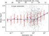 |
Fig. 14 Spectral slope of S types as a function of asteroid diameters (gray points), the weighted average in logarithmic size bins shown by red points. Weights were estimated by color uncertainty. |
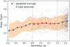 |
Fig. 15 Spectral slope against perihelion for S types. Red dots and the shaded area are the running average and deviation, and blue lines are linear regressions on the running average. Although the entire sample presents a large spread, the running average shows two kinks. |
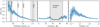 |
Fig. 16 Running mean of the ratio between the number of Q and S asteroids as a function of perihelion, inclination, and diameter. Shaded areas correspond to the uncertainties considering Poisson statistic for the Q/S ratio. |
 |
Fig. 17 Running mean of the ratio between the number of Q and S asteroids as a function of their MOID with the Earth, Venus, and Mars. |
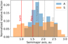 |
Fig. 18 Relative distribution of A-types along the semi-major axis. |
5.2 Distribution of A types
A types are a rare type of asteroids in the Main Belt. Their spectra exhibit a broad and deep absorption band around 1 μm, indicating an olivine-rich composition (e.g., Rivkin et al. 2007). They have been thought to originate from the mantle of differentiated planetesimals (Cruikshank & Hartmann 1984), leading to the “missing mantle issue” (Burbine et al. 1996). The origin of A types is still debated (Sanchez et al. 2014; DeMeo et al. 2019), although, the study of Mars Trojans indicates that certain A-type asteroids could be fragments that were ejected from Mars (Polishook et al. 2017; Christou et al. 2021).
The fraction of A-type asteroids by number in the entire Main Belt is estimated at about 0.16% and are believed to be homogeneously distributed (DeMeo et al. 2019). We report here a fraction of 2.5 ± 0.2% A types among NEOs (focusing on classifications with a probability higher than 0.5). This much higher fraction of A types has already been reported by both the MANOS and NEOSHIELD-2 surveys (Fig. 11, from 1.7 to 5.5%, Popescu et al. 2018b; Devogèle et al. 2019). While a classification based on visible wavelengths only may overestimate the fraction of A (misclassified from red S types owing to space weathering or observations at high phase angles, Sanchez et al. 2012), the fraction of A types among NEOs appears to be an order of magnitude higher than in the Main Belt. Finally, Devogèle et al. (2019) reported a concentration of A types with a semi major axis close to that of Mars (1.5 AU).
We present in Fig. 18 the fraction of A- and S-type NEOs as a function of semi major axis. While S types are evenly distributed, A types are concentrated between the orbit of Mars and the 4:1 resonance with Jupiter, similar to the report by Devogèle et al. (2019). Most A-type NEOs seem to be related to the Hungarias. In this region, the fraction of A-type asteroids increase by up to 4%. So, while the majority of the Hungarias are C and E types (DeMeo & Carry 2014; Lucas et al. 2019), approximately 3% of asteroids in this region are A types.
5.3 The dependence of asteroid colors on phase angle
The color of an asteroid is determined by the light it reflects, which is influenced by the composition of its surface material. However, the observed color of an asteroid can also change with the phase angle, which is the angle between the observer (usually Earth), the asteroid, and the Sun (Belskaya & Shevchenko 2000; Waszczak et al. 2015). This change in color with phase angle is likely due to the way light scatters off the asteroid’s surface. At higher phase angles, the light we see is more likely to have been scattered multiple times within the asteroid’s surface before being reflected back to us. This multiple scattering can cause a redder object to appear bluer and vice versa, although this effect is only noticeable for phase angles of less than 7.5 degrees (Alvarez-Candal et al. 2022b). Considering the change in asteroid color with phase angle can be important for accurate taxonomy classification using color analysis techniques (Colazo et al. 2022).
However, the exact mechanisms behind this color change with phase angle are still not fully understood and are an active area of research. The shape of the asteroid, its rotational state, and the macroscopic roughness of its surface can also influence the observed color and its change with phase angle (Carvano & Davalos 2015).
To investigate the impact of the phase effect on asteroid colors, we compared both the SDSS and SMSS data sets with the absolute magnitude colors from the study by Alvarez-Candal et al. (2022a). The histograms of the g-i difference between the two data sets are shown in Fig. 19.
We also selected asteroids that were observed at phase angles of greater than 20 degrees and had a phase difference of more than 5 degrees between observations. Subsequently, we determined the slope of the asteroid’s g-i color as a function of phase angle. We found that color slope changes randomly and is comparable to the uncertainties in color.
To investigate the trends among “red” and “blue” asteroids, we subdivided the asteroid data set into two groups based on their g-i colors. A red group is indicative of silicate asteroids, and a blue group is representative of carbonaceous asteroids. With this analysis, we did not catch any trends toward reddening or bluing within these subsets. The random behavior of asteroid color slope indicates that more significant factors, such as the shape of the asteroid and uncertainties in photometry, may have a greater influence on the observed color and consequently on asteroid taxonomy.
Given that the phase effect could significantly alter the colors of asteroids only at large phase angles, and considering that our sample does not include NEOs observed at phase angles exceeding 40 degrees, we conclude that we cannot precisely predict and then correct the phase effect. Therefore, we did not take the phase effect into account in the color analysis of the NEOs data set.
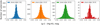 |
Fig. 19 Distribution of the difference between the SDSS g-i asteroid colors and absolute magnitude (H) colors from Alvarez-Candal et al. (2022a) as a function of phase angle. |
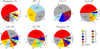 |
Fig. 20 Taxonomic distribution of NEAs as per the seven-region model, previously calculated by Granvik et al. (2018). |
5.4 Source regions
Investigating the orbital and size characteristics, as well as the origin of NEOs, is a crucial area of research in planetary sciences (Binzel et al. 2015; Abell et al. 2015). The dynamical pathway from the source regions to the planet-crossing space is a crucial foundation for studying both individual NEAs and broader population-level questions. Understanding these distributions gives a holistic understanding of the dynamics, origins, and potential risks associated with NEAs.
To deduce the probable origins of NEAs, we relied on what is known of their orbital properties in conjunction with previously simulated probabilities of seven-region7 escape regions by Granvik et al. (2018). We assigned each asteroid to its most probable origin area by employing a three-dimensional grid of orbital elements and a value of absolute magnitude as the fourth parameter. The grid includes semi major axis, a, eccentricity, e, and inclination, i, which was predicated on the calculations previously detailed in the research of Granvik et al. (2018). The orbital elements of these celestial bodies were obtained from the Minor Planet Center (MPC) database.
The most abundant source of NEOs is the ν6, which limits the inner border of the Main Belt. We predict it to be dominated by mafic-silicate-rich asteroids (S, Q, V, see Fig. 20). The distribution of taxonomic classes is almost similar for the other source regions in the inner belt: the 3:1 MMR limiting the inner and middle belt, and the Phocaea and Hungaria regions. The fraction of mafic-silicate-rich asteroids decreases for source regions located further from the Sun (5:2 and 2:1 MMR, JFC). These are dominated by opaque-rich asteroids (B, C, D, see Fig. 20). Despite the observation biases (mainly related to albedo) and the relative low number of NEOs predicted to originate from the outer regions, our results are in close agreement with Marsset et al. (2022), in line with the current understanding of taxonomic distribution (DeMeo & Carry 2014), but in a smaller size range.
6 Conclusions
We combined a large sample of colors of planet-crossing asteroids, combining broadband photometry from the SDSS and SMSS surveys and reflectance spectroscopy from the ESA Gaia mission and ground-based observations. We determined the taxonomy of 7401 NEOs, with diameters from approximately 10 km to 50 m. The sample is dominated by S-type asteroids (approximately 45%), as occurs for other NEOs surveys. However, it is notable that the proportion of S types is overestimated due to observational bias. We also report a much higher (up to 4%) fraction of A types among NEOs as compared to the Main Belt. These A types are concentrated on a semi major axis between 1.5 and 2 AU. We confirm a strong dependence of the spectral slope of S types with perihelion, based on a sample of over one thousand objects. The distribution of slope is consistent with the recently proposed rejuvenation model through thermal fatigue.
Acknowledgements
This research has been conducted within the NEOROCKS project, which has received funding from the European Union’s Horizon 2020 research and innovation programme under grant agreement No 870403. The NEOROCKS team is composed by E. Dotto, M. Banaszkiewicz, S. Banchi, M.A. Barucci, F. Bernardi, M. Birlan, A. Cellino, J. De Leon, M. Lazzarin, E. Maz-zotta Epifani, A. Mediavilla, D. Perna, E. Perozzi, P. Pravec, C. Snodgrass, C. Teodorescu, S. Anghel, A. Bertolucci, F. Calderini, F. Colas, A. Del Vigna, A. Dell’Oro, A. Di Cecco, L. Dimare, I. Di Pietro, P. Fatka, S. Fornasier, E. Frattin, P. Frosini, M. Fulchignoni, R. Gabryszewski, M. Giardino, A. Giunta, T. Hromakina, J. Huntingford, S. Ieva, J.P. Kotlarz, F. La Forgia, J. Lican-dro, H. Medeiros, F. Merlin, J. Nomen Torres, V. Petropoulou, F. Pina, G. Polenta, M. Popescu, A. Rozek, P. Scheirich, A. Sonka, G.B. Valsecchi, P. Wajer, A. Zinzi. This research has made use of the SVO Filter Profile Service supported from the Spanish MINECO through grant AYA2017-84089 (Rodrigo et al. 2012; Rodrigo & Solano 2020). We did an extensive use of the Virtual Observatory (VO) TOPCAT software (Taylor 2005), and IMCCE’s VO tools SkyBot (Berthier et al. 2006) and SsODNet (Berthier et al. 2023). This work made use of Astropy (http://www.astropy.org) a community-developed core Python package and an ecosystem of tools and resources for astronomy (Astropy Collaboration 2013, 2018, 2022). This research made use of Photutils, an Astropy package for detection and photometry of astronomical sources (Bradley et al. 2020). Thanks to all the developers and maintainers. This work has made use of data from the European Space Agency (ESA) mission Gaia (https://www.cosmos.esa.int/gaia), processed by the Gaia Data Processing and Analysis Consortium (DPAC, https://www.cosmos.esa.int/web/gaia/dpac/consortium). Funding for the DPAC has been provided by national institutions, in particular the institutions participating in the Gaia Multilateral Agreement. Funding for SDSS-III has been provided by the Alfred P. Sloan Foundation, the Participating Institutions, the National Science Foundation, and the U.S. Department of Energy Office of Science. The SDSS-III web site is http://www.sdss3.org. SDSS-III is managed by the Astrophysical Research Consortium for the Participating Institutions of the SDSS-III Collaboration including the University of Arizona, the Brazilian Participation Group, Brookhaven National Laboratory, Carnegie Mellon University, University of Florida, the French Participation Group, the German Participation Group, Harvard University, the Instituto de Astrofisica de Canarias, the Michigan State/Notre Dame/JINA Participation Group, Johns Hopkins University, Lawrence Berkeley National Laboratory, Max Planck Institute for Astrophysics, Max Planck Institute for Extraterrestrial Physics, New Mexico State University, New York University, Ohio State University, Pennsylvania State University, University of Portsmouth, Princeton University, the Spanish Participation Group, University of Tokyo, University of Utah, Vanderbilt University, University of Virginia, University of Washington, and Yale University.
Appendix A Conversion of reflectance to color
A common strategy used to improve the detection of com-positionally similar dependences in data analysis is to reduce the data’s dimensionality. This process involves simplifying the data without losing critical information. When working with reflectance spectra that cover the same wavelength range, they can be transformed into colors, under the condition that the data encompass similarly broad wavelength ranges. This conversion facilitates better visualization and comparison of our data.
The transformation procedure involves several steps. Initially, each reflectance value was multiplied by a solar spectrum, which was taken from Bohlin et al. (2014) and the filter transmission curves. The solar spectrum was used because it is the light from the Sun that is being reflected off the surfaces of the asteroids. The filter transmission curves were used to mimic the response of the instrument that would be observing this reflected light. Once these multiplications were completed, we calculated the integrals by summing up all of the individual product values across the wavelength range to produce a single, complete value that characterizes the source photometry value in the filter. This process is detailed in (Chap. 7 in IMCCE 2021). The color index value is the logarithm relation of photometry obtained in two filters, which provides a measure of the object’s color.
We have two types of reflectance spectra under consideration. The Gaia reflectance spectra consist of 16 data points, each a measurement of how much light an asteroid reflects at specific wavelengths. These values span from 374 nm to 1034 nm, increasing by 44 nm increments. The Classy reflectance spectra are more extensive, comprising 53 tabulated values ranging from 0.45 μm to 2.45 μm. The intervals between these values are 0.025 μm up to 1.025 μm, and increase to 0.05 μm beyond this point.
We note that not all data from the Gaia spectra are reliable. Specifically, the first two values (which represent blue light) and the last two values (representing red light) can sometimes be inaccurate or spurious. Although these suspect values are often flagged in the Gaia DR3 catalog (Gaia Collaboration 2023b), this is not always the case. To address this problem, we discarded these unreliable values and replaced them with extrapolated values. This extrapolation was based on the trend observed in the three nearest (and more reliable) reflectance values, as illustrated in (Fig. A.1).
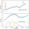 |
Fig. A.1 Examples of Gaia reflectance spectra of the asteroid (376817) 2001 AT43 (top) and Classy reflectance of the asteroid (4688) 1980 WF (bottom). Red points indicate outliers (see Gaia Collaboration 2023b), while gray points indicate extrapolated values (see text). We overplot the transmission curves of the SDSS g, r, i, and z filters to show the wavelength range covered by the reflectance spectra. |
Having carried out these preliminary steps, we proceeded to convert the refined reflectance spectra into standard color indexes used in astronomy, namely g-r, g-i, r-i, and i-z colors. This transformation is undertaken within the photometric system of the SDSS, a major astronomical survey that has provided extensive data on the night sky. To ensure accuracy in this conversion, we retrieved the transmission curves of the SDSS filters from the SVO filter profile service8. This service contains a variety of transmission curves from a multitude of observatories and astronomical instruments (Rodrigo et al. 2012; Rodrigo & Solano 2020).
Finally, we calculated the uncertainties associated with these color values. These uncertainties provide a measure of the potential error or variability in our color measurements. They are calculated as half the difference of color computed using the reflectance, plus and minus uncertainties. This gives us a measure of the range within which the true color value is likely to lie, thereby providing us with a more comprehensive understanding of the asteroids’ color data.
Appendix B Photometry of fast-moving targets
The apparent motion of Main Belt asteroids is typically about 40 ″/h. The length of the streak during the exposure (54 s) is thus comparable with the typical seeing of SDSS images. However, NEOs have significantly faster apparent motion, up to hundreds of arcseconds per hour, leading to trailed signatures (Fig. B.1, Solano et al. (2014)).
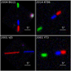 |
Fig. B.1 Examples of fast-moving NEOs in SDSS images. The color images are a combination of FITS images in g (green), r (red), and i (blue) filters. |
Through visual inspection of random NEOs images from the SDSS database, and checking their photometry from the SDSS pipeline (as reported by Sergeyev & Carry 2021), we found that fast-moving NEOs sometimes have incorrect photometry. This is likely because they were not recognized as a single object in the different filters by the SDSS pipeline. Furthermore, the SDSS PSF photometry of elongated NEO tracks is biased. We finally identified a few cases of erroneous estimate of the zero-point in individual SDSS Flexible Image Transport System (FITS) frames. We note that SDSS magnitudes are expressed as inverse hyperbolic sines (“asinh” magnitudes, Lupton et al. 1999). They are virtually identical to the usual Pogson astronomical magnitude in the high signal-to-noise ratio (S/N) regime, but can diverge for faint objects such as NEOs.
We overcame these issues by remeasuring the photometry of NEOs moving faster than 80 ″/h on SDSS images. We selected 470 NEOs with either an expected S/N above 10 in the z filter or multiple measurements. We used these criteria to ensure meaningful colors for taxonomy: typical color differences between classes are on the order of 0.1 mag (DeMeo & Carry 2013), and the z filter is crucial for probing the presence of an absorption band around 1 μm (Carry et al. 2016), which has been one of the major discriminants in all taxonomies for the past half a century (Chapman et al. 1975).
For this task, we developed a python software using the astropy (Astropy Collaboration 2013, 2018, 2022) photoutils (Bradley et al. 2020), astroquery (Ginsburg et al. 2019), and sep (the core algorithms of SExtractor, Bertin & Arnouts 1996; Barbary 2016) packages. The procedure to measure the photometry encompassed the following steps.
First, we estimated the zero-point value of each SDSS frame. We identified non-saturated bright stars and measured their instrumental magnitude with aperture photometry. We then derived the slope and zero-point of individual frames by comparing these values with the photometry from the SDSS PhotoPrimary catalog (York et al. 2000), which contains only stationary sources.
Using the sep package, we identified all sources in cutout images centered on the predicted location of the asteroid. The SDSS images in different filters were obtained sequentially, with a delay of 17.7 s between each of the 54 s exposures. The position of the cut-out image of the asteroid hence changes in each filter, with the largest shift occuring between filters g and r. Therefore, we identified the NEOs in these two filters using SkyBoT (Berthier et al. 2006, Berthier et al. 2016), since it provides the best S/N and brackets the other observations. We then predicted the NEOs positions in other filters based on these determinations. We next checked the images visually to select only those NEOs not blended with stars. Whenever a NEO was observed on multiple epochs, we co-added the asteroid-centered cut-out images to increase the asteroid S/N prior to measuring its photometry.
We finally measured the magnitude of each NEO in each filter using an elliptical aperture to account for the PSF elongation due to the fast motion (Fig. B.2). We illustrate the improvement on the photometry in Fig. B.3. These updated magnitudes are the ones used in the creation of the NEOROCKS data set.
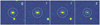 |
Fig. B.2 Photometry of 2006 UA on SDSS images, illustrating the elliptical aperture. The inner ellipse shows the region in which photons are counted. The two outer circles show the annulus used to estimate the sky background. |
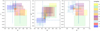 |
Fig. B.3 Colors of (277958) 2006 SP134 from individual SDSS catalog values (in blue) and from our elliptical photometry (orange). The color boxes represent the limits of taxonomic classes. |
Appendix C Estimation of color uncertainties
In order to select the optimal color value amongst multiple catalogs, we had to take into account color value uncertainty. Nevertheless, there may be situations where the reported photometric errors, calculated via diverse methodologies, do not align. For instance, such discrepancies can arise when uncertainties are quantified as either standard deviations or standard errors, particularly when these uncertainties do not follow a normal distribution.
The availability of color estimates for the same asteroids in the different catalogs allowed us to compare the difference in color distribution with photometric uncertainties. Color indexes, such as the g-r index, represent the difference in magnitude (brightness) between two different wavelength bands for a given object. Uncertainties in these indices can be calculated from the uncertainties in the photometric measurements for each band.
For example, in the g-r color index, the uncertainty can be calculated from the errors in the g and r magnitudes. For two different catalogs, we could represent these calculations as follows:

Here,  and
and  are the uncertainties of the g and r photometry from the first catalog, and g2err and r2err are the uncertainties from the second catalog. If we assume that the color of an asteroid does not change over time, we can calculate the difference in the color indices measured in two different catalogs. This can be done using the previously computed uncertainties:

where Δ(gr1 – gr2) is the difference in the g-r color index between the two catalogs and gr1err and gr2err are the uncertainties of this color index in the first and second catalogs, respectively.
Estimating the uncertainty of stellar objects is a complex task. While internal errors could provide a reasonable uncertainty estimate, systematic errors may distort these results. It is important to keep in mind that published uncertainties may potentially contain distortions that have not been accounted for. If we consider that the published uncertainties might not be accurate, and the true uncertainties are gr1err * k1 and gr2err * k2, where k1 and k2 are unknown factors, in this case, the difference in the color indices can be calculated as

In instances where there are more than two catalogs at our disposal, we can calculate the color difference between each pair of catalogs. For example, if we have three catalogs, we can formulate the following:

This formulation provides us with a system of three equations featuring three unknown variables (k1, k2, and k3). These equations can be resolved in order to estimate the authentic uncertainties inherent to each catalog.
In situations involving four catalogs (for instance, SDSS, SMSS, Gaia, and Classy, in our example), we can compute the color differences between every pair, resulting in a system of six equations with four unknowns. This system is generally resolved using a least squares method. The solutions derived from this system would produce the estimated authentic uncertainties associated with each catalog.
We extracted the common asteroids from each of our four catalogs and obtained three samples for each of them. For example, for the SDSS catalog, we obtained SMSS, Gaia, and Classy cross-match samples that contain 54 283 27158, and 1807 of common asteroids, correspondingly. Cumulative distributions of color errors for four colors are presented in Figure C.1, where we can see the typical photometry error distribution of the SDSS and SkyMapper data that are limited by the magnitude. While the Gaia errors have a uniform distribution because the data have no dependence on the asteroid magnitude, the Classy data have no information about their errors, and therefore we generated random uniform errors in the range from 0 to 0.1 magnitudes.
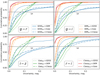 |
Fig. C.1 Cumulative distributions of the difference of color for asteroids in SDSS and the rest of the catalogs (blue), as well as their color uncertainties obtained from photometry (orange). |
The variation between the three distributions of the same catalog errors shows a different composition of the common samples. The correction coefficients of color uncertainties for each catalog, calculated using the least squares method, are presented in Table C.1.
Correction factors for catalog color uncertainty estimates.
We subsequently calculated the cumulative distribution of color differences between asteroids found in varying catalogs. In Figure C.2, we depict the declared cumulative error distribution of each catalog. It is observable that the distribution of the declared SMSS color uncertainties is overestimated compared with the computed distribution, especially within the SMSS ⋂ SDSS sample. Conversely, the Gaia uncertainties seem to be underestimated, possibly owing to the manner in which we computed the uncertainties during the derivation of the color.
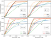 |
Fig. C.2 Cumulative distribution of the color uncertainty of asteroids present in SDSS SMSS, Gaia, and Classy samples. Vertical lines indicate the estimated values of color index difference errors. |
Appendix D Vikiri spectrum
We present a near-infrared spectrum of (10278) Virkki in Figure D.1. This spectrum was collected with the 3-m IRTF located on Maunakea, Hawaii, on October 14, 2020, through the MITH-NEOS program (Binzel et al. 2019, PI: DeMeo). We used the SpeX NIR spectrograph (Rayner et al. 2003) combined with a 0.8×15″ slit in the low-resolution prism mode to measure the spectra over the 0.7-2.5 μm wavelength range. Asteroid observations were bracketed with measurements of the following calibration stars, which are known to be very close spectral analogs to the Sun: Hyades 64 and Landolt (1983) stars 93101 and 113-276. In-depth analysis of these calibration stars and additional stars used in MITHNEOS is provided in Marsset et al. (2020). Data reduction and spectral extraction followed the procedure outlined in Binzel et al. (2019), with the Autospex software tool (Rivkin et al. 2005).
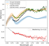 |
Fig. D.1 Near-infrared spectrum of (10278) Virkki (black dots), a former candidate for flyby by the ESA Hera mission. The orange line is the S-type asteroid spectrum template from Mahlke et al. (2022). Their ratio is typical of space weathering (red points in the bottom panel). Blue points present the reflectance corrected by the space weathering. |
These steps included trimming the images, creating a bad pixel map, flat-fielding the images, sky subtraction, tracing the spectra in both the wavelength and spatial dimensions, co-adding the spectral images, extracting the spectra, performing wavelength calibration, and correcting for air-mass differences between the asteroids and the corresponding solar analogs. The resulting asteroid spectra were divided by the mean stellar spectra to remove the solar gradient.
Appendix E Catalog description
We describe here the catalog of the NEAs we have released. The catalog contains four colors (g-r, g-i, r-i, and i-z), osculating elements, the most probable taxonomy, and the source region for each asteroid. The catalog presented here is available at the CDS.
Description of catalog that includes obtained colors, taxonomy, and orbital elements of NEOs.
References
- Abell, P., Barbee, B. W., Mink, R. G., et al. 2012, in AAS/Division for Planetary Sciences Meeting Abstracts, 44 [Google Scholar]
- Abell, P. A., Barbee, B. W., Chodas, P. W., et al. 2015, in Asteroids IV, 855 [Google Scholar]
- Agostini, L., Lucchetti, A., Pajola, M., et al. 2022, Planet. Space Sci., 216, 105476 [NASA ADS] [CrossRef] [Google Scholar]
- Alvarez-Candal, A., Benavidez, P. G., Campo Bagatin, A., & Santana-Ros, T. 2022a, A & A, 657, A80 [NASA ADS] [CrossRef] [EDP Sciences] [Google Scholar]
- Alvarez-Candal, A., Jimenez Corral, S., & Colazo, M. 2022b, A & A, 667, A81 [NASA ADS] [CrossRef] [EDP Sciences] [Google Scholar]
- Astropy Collaboration (Robitaille, T. P., et al.) 2013, A & A, 558, A33 [NASA ADS] [CrossRef] [EDP Sciences] [Google Scholar]
- Astropy Collaboration (Price-Whelan, A. M., et al.) 2018, AJ, 156, 123 [Google Scholar]
- Astropy Collaboration (Price-Whelan, A. M., et al.) 2022, ApJ, 935, 167 [NASA ADS] [CrossRef] [Google Scholar]
- Barbary, K. 2016, J. Open Source Softw., 1, 58 [Google Scholar]
- Belskaya, I. N., & Shevchenko, V. G. 2000, Icarus, 147, 94 [NASA ADS] [CrossRef] [Google Scholar]
- Belskaya, I., Cellino, A., Gil-Hutton, R., Muinonen, K., & Shkuratov, Y. 2015, in Asteroids IV, 151 [Google Scholar]
- Belton, M. J. S., Chapman, C. R., Thomas, P. C., et al. 1995, Nature, 374, 785 [NASA ADS] [CrossRef] [Google Scholar]
- Berthier, J., Vachier, F., Thuillot, W., et al. 2006, ASP Conf. Ser., 351, 367 [NASA ADS] [Google Scholar]
- Berthier, J., Carry, B., Vachier, F., Eggl, S., & Santerne, A. 2016, MNRAS, 458, 3394 [NASA ADS] [CrossRef] [Google Scholar]
- Berthier, J., Carry, B., Mahlke, M., & Normand, J. 2023, A & A, 671, A151 [NASA ADS] [CrossRef] [EDP Sciences] [Google Scholar]
- Bertin, E., & Arnouts, S. 1996, A & AS, 117, 393 [NASA ADS] [Google Scholar]
- Binzel, R. P., Rivkin, A. S., Stuart, J. S., et al. 2004, Icarus, 170, 259 [NASA ADS] [CrossRef] [Google Scholar]
- Binzel, R. P., Morbidelli, A., Merouane, S., et al. 2010, Nature, 463, 331 [NASA ADS] [CrossRef] [Google Scholar]
- Binzel, R. P., Reddy, V., & Dunn, T. 2015, Asteroids IV, 243 [Google Scholar]
- Binzel, R. P., DeMeo, F. E., Turtelboom, E. V., et al. 2019, Icarus, 324, 41 [Google Scholar]
- Bohlin, R. C., Gordon, K. D., & Tremblay, P. E. 2014, PASP, 126, 711 [NASA ADS] [Google Scholar]
- Bradley, L., Sipőcz, B., Robitaille, T., et al. 2020, https://zenodo.org/records/4044744 [Google Scholar]
- Brunetto, R., Vernazza, P., Marchi, S., et al. 2006, Icarus, 184, 327 [CrossRef] [Google Scholar]
- Brunetto, R., Loeffler, M. J., Nesvorný, D., Sasaki, S., & Strazzulla, G. 2015, Asteroid Surface Alteration by Space Weathering Processes, eds. P. Michel, F. DeMeo, & W. F. Bottke, 597 [Google Scholar]
- Burbine, T. H., Meibom, A., & Binzel, R. P. 1996, Meteor. Planet. Sci., 31, 607 [NASA ADS] [CrossRef] [Google Scholar]
- Bus, S. J., & Binzel, R. P. 2002, Icarus, 158, 106 [CrossRef] [Google Scholar]
- Carry, B. 2018, A & A, 609, A113 [NASA ADS] [CrossRef] [EDP Sciences] [Google Scholar]
- Carry, B., Kaasalainen, M., Leyrat, C., et al. 2010, A & A, 523, A94 [NASA ADS] [CrossRef] [EDP Sciences] [Google Scholar]
- Carry, B., Solano, E., Eggl, S., & DeMeo, F. 2016, Icarus, 268, 340 [CrossRef] [Google Scholar]
- Carvano, J. M., & Davalos, J. A. G. 2015, A & A, 580, A98 [NASA ADS] [CrossRef] [EDP Sciences] [Google Scholar]
- Cellino, A., Bendjoya, P., Delbo’, M., et al. 2020, A & A, 642, A80 [NASA ADS] [CrossRef] [EDP Sciences] [Google Scholar]
- Chapman, C. R. 2004, Annu. Rev. Earth Planet. Sci., 32, 539 [CrossRef] [Google Scholar]
- Chapman, C. R., Morrison, D., & Zellner, B. H. 1975, Icarus, 25, 104 [NASA ADS] [CrossRef] [Google Scholar]
- Chapman, C. R., Veverka, J., Thomas, P. C., et al. 1995, Nature, 374, 783 [NASA ADS] [CrossRef] [Google Scholar]
- Christou, A. A., Borisov, G., Dell’Oro, A., Cellino, A., & Devogèle, M. 2021, Icarus, 354, 113994 [NASA ADS] [CrossRef] [Google Scholar]
- Cloutis, E. A., Sanchez, J. A., Reddy, V., et al. 2015, Icarus, 252, 39 [NASA ADS] [CrossRef] [Google Scholar]
- Colazo, M., Alvarez-Candal, A., & Duffard, R. 2022, A & A, 666, A77 [NASA ADS] [CrossRef] [EDP Sciences] [Google Scholar]
- Consolmagno, G., Britt, D., & Macke, R. 2008, Chem. Erde/Geochemistry, 68, 1 [NASA ADS] [Google Scholar]
- Cruikshank, D. P., & Hartmann, W. K. 1984, Science, 223, 281 [NASA ADS] [CrossRef] [Google Scholar]
- Delbo, M., Libourel, G., Wilkerson, J., et al. 2014, Nature, 508, 233 [Google Scholar]
- DeMeo, F. E., & Carry, B. 2013, Icarus, 226, 723 [NASA ADS] [CrossRef] [Google Scholar]
- DeMeo, F., & Carry, B. 2014, Nature, 505, 629 [NASA ADS] [CrossRef] [Google Scholar]
- DeMeo, F., Binzel, R. P., Slivan, S. M., & Bus, S. J. 2009, Icarus, 202, 160 [NASA ADS] [CrossRef] [Google Scholar]
- DeMeo, F. E., Polishook, D., Carry, B., et al. 2019, Icarus, 322, 13 [CrossRef] [Google Scholar]
- DeMeo, F. E., Marsset, M., Polishook, D., et al. 2023, Icarus, 389, 115264 [NASA ADS] [CrossRef] [Google Scholar]
- Devogèle, M., Moskovitz, N., Thirouin, A., et al. 2019, AJ, 158, 196 [CrossRef] [Google Scholar]
- Di Martino, M., Ferreri, W., Fulchignoni, M., et al. 1990, Icarus, 87, 372 [NASA ADS] [CrossRef] [Google Scholar]
- Doressoundiram, A., Weissman, P. R., Fulchignoni, M., et al. 1999, A & A, 352, 697 [NASA ADS] [Google Scholar]
- Dotto, E., Banaszkiewicz, M., Banchi, S., et al. 2021, in 7th IAA Planetary Defense Conference, 221 [Google Scholar]
- Drube, L., Harris, A. W., Hoerth, T., et al. 2015, in Handbook of Cosmic Hazards and Planetary Defense, 763 [CrossRef] [Google Scholar]
- Erasmus, N., Navarro-Meza, S., McNeill, A., et al. 2020, ApJS, 247, 13 [CrossRef] [Google Scholar]
- Fitzsimmons, A., Khan, M., Küppers, M., Michel, P., & Pravec, P. 2020, in European Planetary Science Congress, EPSC2020-1064 [Google Scholar]
- Fujiwara, A., Kawaguchi, J., Yeomans, D. K., et al. 2006, Science, 312, 1330 [NASA ADS] [CrossRef] [Google Scholar]
- Gaia Collaboration (Prusti, G., et al.) 2016, A & A, 595, A1 [NASA ADS] [CrossRef] [EDP Sciences] [Google Scholar]
- Gaia Collaboration (Vallenari, et al.) 2023a, A & A, 674, A1 [NASA ADS] [CrossRef] [EDP Sciences] [Google Scholar]
- Gaia Collaboration (Galluccio, L., et al.) 2023b, A & A, 674, A35 [NASA ADS] [CrossRef] [EDP Sciences] [Google Scholar]
- Ginsburg, A., Sipőcz, B. M., Brasseur, C. E., et al. 2019, AJ, 157, 98 [Google Scholar]
- Gladman, B. J., Migliorini, F., Morbidelli, A., et al. 1997, Science, 277, 197 [NASA ADS] [CrossRef] [Google Scholar]
- Gounelle, M., Spurný, P., & Bland, P. A. 2006, Meteor. Planet. Sci., 41, 135 [NASA ADS] [CrossRef] [Google Scholar]
- Granvik, M., & Brown, P. 2018, Icarus, 311, 271 [Google Scholar]
- Granvik, M., Morbidelli, A., Jedicke, R., et al. 2018, Icarus, 312, 181 [CrossRef] [Google Scholar]
- Graves, K., Minton, D., Hirabayashi, M., DeMeo, F., & Carry, B. 2018, Icarus, 304, 162 [CrossRef] [Google Scholar]
- Graves, K. J., Minton, D. A., Molaro, J. L., & Hirabayashi, M. 2019, Icarus, 322, 1 [NASA ADS] [CrossRef] [Google Scholar]
- Harris, A. W., & Lagerros, J. S. V. 2002, in Asteroids III, 205 [Google Scholar]
- IMCCE 2021, Introduction aux éphémérides et phénomènes astronomiques, eds. J. Berthier, P. Descamps, & F. Mignard (EDP Sciences) [Google Scholar]
- Küppers, M., O’Rourke, L., Bockelée-Morvan, D., et al. 2014, Nature, 505, 525 [CrossRef] [Google Scholar]
- Landolt, A. U. 1983, AJ, 88, 439 [Google Scholar]
- Lantz, C., Brunetto, R., Barucci, M. A., et al. 2017, Icarus, 285, 43 [CrossRef] [Google Scholar]
- Lantz, C., Binzel, R. P., & DeMeo, F. 2018, Icarus, 302, 10 [CrossRef] [Google Scholar]
- Lauretta, D. S., Balram-Knutson, S. S., Beshore, E., et al. 2017, Space Sci. Rev., 212, 925 [Google Scholar]
- Lazzarin, M., Marchi, S., Barucci, M. A., di Martino, M., & Barbieri, C. 2004, Icarus, 169, 373 [NASA ADS] [CrossRef] [Google Scholar]
- Lazzarin, M., Marchi, S., Magrin, S., & Licandro, J. 2005, MNRAS, 359, 1575 [Google Scholar]
- Lucas, M. P., Emery, J. P., MacLennan, E. M., et al. 2019, Icarus, 322, 227 [NASA ADS] [CrossRef] [Google Scholar]
- Lupton, R. H., Gunn, J. E., & Szalay, A. S. 1999, AJ, 118, 1406 [Google Scholar]
- Mahlke, M., Carry, B., & Mattei, P. A. 2022, A & A, 665, A26 [NASA ADS] [CrossRef] [EDP Sciences] [Google Scholar]
- Marchi, S., Paolicchi, P., & Richardson, D. C. 2012, MNRAS, 421, 2 [NASA ADS] [Google Scholar]
- Marsset, M., DeMeo, F. E., Binzel, R. P., et al. 2020, ApJS, 247, 73 [NASA ADS] [CrossRef] [Google Scholar]
- Marsset, M., DeMeo, F. E., Burt, B., et al. 2022, AJ, 163, 165 [NASA ADS] [CrossRef] [Google Scholar]
- Masiero, J. R., Wright, E. L., & Mainzer, A. K. 2021, PSJ, 2, 32 [NASA ADS] [Google Scholar]
- McSween, H. Y., Lauretta, D. S., & Leshin, L. A. 2006, Meteorites and the Early Solar System II, 53 [CrossRef] [Google Scholar]
- Michel, P., Küppers, M., Bagatin, A. C., et al. 2022, PSJ, 3, 160 [NASA ADS] [Google Scholar]
- Nesvorný, D., Jedicke, R., Whiteley, R. J., & Ivezić, Z. 2005, Icarus, 173, 132 [CrossRef] [Google Scholar]
- Nesvorný, D., Bottke, W. F., Vokrouhlicky, D., Chapman, C. R., & Rafkin, S. 2010, Icarus, 209, 510 [CrossRef] [Google Scholar]
- Noguchi, T., Nakamura, T., Kimura, M., et al. 2011, Science, 333, 1121 [NASA ADS] [CrossRef] [Google Scholar]
- Parker, A., Ivezić, Ž., Jurić, M., et al. 2008, Icarus, 198, 138 [Google Scholar]
- Perna, D., Barucci, M. A., Fulchignoni, M., et al. 2018, Planet. Space Sci., 157, 82 [CrossRef] [Google Scholar]
- Polishook, D., Jacobson, S. A., Morbidelli, A., & Aharonson, O. 2017, Nat. Astron., 1, 0179 [NASA ADS] [CrossRef] [Google Scholar]
- Popescu, M., Licandro, J., Carvano, J. M., et al. 2018a, A & A, 617, A12 [NASA ADS] [CrossRef] [EDP Sciences] [Google Scholar]
- Popescu, M., Perna, D., Barucci, M. A., et al. 2018b, MNRAS, 477, 2786 [NASA ADS] [CrossRef] [Google Scholar]
- Rayner, J. T., Toomey, D. W., Onaka, P. M., et al. 2003, PASP, 115, 362 [NASA ADS] [CrossRef] [Google Scholar]
- Reddy, V., Dunn, T. L., Thomas, C. A., Moskovitz, N. A., & Burbine, T. H. 2015, in Asteroids IV, 43 [Google Scholar]
- Rivkin, A. S., Binzel, R. P., & Bus, S. J. 2005, Icarus, 175, 175 [NASA ADS] [CrossRef] [Google Scholar]
- Rivkin, A. S., Trilling, D. E., Thomas, C. A., et al. 2007, Icarus, 192, 434 [NASA ADS] [CrossRef] [Google Scholar]
- Rivkin, A. S., Chabot, N. L., Stickle, A. M., et al. 2021, PSJ, 2, 173 [NASA ADS] [Google Scholar]
- Rodrigo, C., & Solano, E. 2020, in XIV.0 Scientific Meeting (virtual) of the Spanish Astronomical Society, 182 [Google Scholar]
- Rodrigo, C., Solano, E., & Bayo, A. 2012, SVO Filter Profile Service Version 1.0, IVOA Working Draft 15 October 2012 [Google Scholar]
- Ruesch, O., Platz, T., Schenk, P., et al. 2016, Science, 353, aaf4286 [NASA ADS] [CrossRef] [Google Scholar]
- Sanchez, J. A., Reddy, V., Nathues, A., et al. 2012, Icarus, 220, 36 [CrossRef] [Google Scholar]
- Sanchez, J. A., Reddy, V., Kelley, M. S., et al. 2014, Icarus, 228, 288 [CrossRef] [Google Scholar]
- Sasaki, S., Nakamura, K., Hamabe, Y., Kurahashi, E., & Hiroi, T. 2001, Nature, 410, 555 [NASA ADS] [CrossRef] [Google Scholar]
- Scheeres, D. J., McMahon, J. W., Wood, J., et al. 2020, in 51st Annual Lunar and Planetary Science Conference, Lunar and Planetary Science Conference, 1965 [Google Scholar]
- Sergeyev, A. V., & Carry, B. 2021, A & A, 652, A59 [NASA ADS] [CrossRef] [EDP Sciences] [Google Scholar]
- Sergeyev, A. V., Carry, B., Onken, C. A., et al. 2022, A & A, 658, A109 [NASA ADS] [CrossRef] [EDP Sciences] [Google Scholar]
- Solano, E., Rodrigo, C., Pulido, R., & Carry, B. 2014, Astron. Nachr., 335, 142 [NASA ADS] [CrossRef] [Google Scholar]
- Strazzulla, G., Dotto, E., Binzel, R. P., et al. 2005, Icarus, 174, 31 [CrossRef] [Google Scholar]
- Tachibana, S., Sawada, H., Okazaki, R., et al. 2022, Science, 375, 1011 [NASA ADS] [CrossRef] [Google Scholar]
- Taylor, M. B. 2005, ASP Conf. Ser., 347, 29 [Google Scholar]
- Tholen, D. J. 1984, Ph.D. Thesis, University of Arizona, USA [Google Scholar]
- Tholen, D. J. 1989, in Asteroids II, eds. R. P. Binzel, T. Gehrels, & M. S. Matthews, 1139 [Google Scholar]
- Thomas, C. A., Trilling, D. E., & Rivkin, A. S. 2012, Icarus, 219, 505 [NASA ADS] [CrossRef] [Google Scholar]
- Usui, F., Kasuga, T., Hasegawa, S., et al. 2013, ApJ, 762, 56 [Google Scholar]
- Vernazza, P., Binzel, R. P., Rossi, A., Fulchignoni, M., & Birlan, M. 2009, Nature, 458, 993 [NASA ADS] [CrossRef] [Google Scholar]
- Viles, H., Ehlmann, B., Wilson, C. F., et al. 2010, Geophys. Res. Lett., 37, L18201 [NASA ADS] [CrossRef] [Google Scholar]
- Waszczak, A., Chang, C.-K., Ofek, E. O., et al. 2015, AJ, 150, 75 [NASA ADS] [CrossRef] [Google Scholar]
- Yano, H., Fujita, M., Kusumoto, T., et al. 2022, in 44th COSPAR Scientific Assembly, 44, 3264 [NASA ADS] [Google Scholar]
- York, D. G., Adelman, J., Anderson, J., John E., et al. 2000, AJ, 120, 1579 [NASA ADS] [CrossRef] [Google Scholar]
- Yurimoto, H., Abe, K.-I., Abe, M., et al. 2011, Science, 333, 1116 [NASA ADS] [CrossRef] [Google Scholar]
(21) Lutetia (Rosetta), (243) Ida (Galileo), (253) Mathilde (NEAR Shoemaker), (951) Gaspra (Galileo), (2867) Steins (Rosetta), (9969) Braille (Deep Space 1), (5525) Annefrank (Stardust).
(1) Ceres (Dawn), (4) Vesta (Dawn), (433) Eros (NEAR Shoemaker), (4179) Toutatis (Chang’e), (25143) Itokawa (Hayabusa), (65803) Didymos (DART), (134340) Pluto (New Horizons), (162173) Ryugu (Hayabusa2), (486958) Arrokoth (New Horizons), (101955) Bennu (OSIRIS-REx).
Retrieved from the Minor Planet Center (MPC).
ν6 secular resonance, 2:1, 3:1, 5:2, mean-motion resonances (MMR) with Jupiter, high inclination Phocaeas and Hungarias, and Jupiter family comets (JFC).
All Tables
Mean and standard deviation of the color difference between SDSS and the other samples.
Description of catalog that includes obtained colors, taxonomy, and orbital elements of NEOs.
All Figures
|
Fig. 1 Schematic view of the extraction, convertion, and merging of NEOs from SDSS, SMSS, Gaia, and Classy catalogs. |
| In the text | |
|
Fig. 2 Distribution of color differences between the SMSS, Gaia, and Classy with respect to the SDSS data set, using asteroids commonly found in these data sets. The distribution was fitted with a Gaussian curve, represented by the black line. The central gray vertical line denotes the zero offset. |
| In the text | |
|
Fig. 3 Distribution of the orbital elements of the NEOs, color-coded by dynamic class. |
| In the text | |
|
Fig. 4 Distribution of absolute magnitude of MCs (blue) and NEAs (orange). The diameter scale is a guideline, computed with an average albedo of 0.24. |
| In the text | |
|
Fig. 5 Color-color distribution NEOs with a taxonomy probability above 0.2, color-coded by taxonomic classes. |
| In the text | |
|
Fig. 6 Pseudo-reflectance spectra of asteroids based on their g-r, g-i, and i-z colors. The distribution of values for each band is represented by whiskers (95% extrema, and the 25, 50, and 75% quartiles). For each class, we also represent the associated template spectra of the Mahlke et al. (2022) taxonomy. |
| In the text | |
|
Fig. 7 Distribution of g-r colors in SDSS asteroids and taxonomic categorization of NEOs. Top: Color distribution of one million asteroids obtained from the SDSS (Sergeyev & Carry 2021) data set modeled by fitting a mixture of two Gaussians (represented by the black line). The two main taxonomic classes, silicate (depicted in orange) and carbonaceous (depicted in blue), were represented by the model. Bottom: Distribution of g-r colors and the taxonomy of NEOs analyzed using the two-component mixture model of the two primary classes in the SDSS data set (shown by lines). The carbonaceous and silicate taxonomy complexes are represented by blue and orange, respectively. Unclassified asteroids, where the probability of belonging to each complex is comparable, are represented in gray. |
| In the text | |
|
Fig. 8 Confusion matrix illustrating the correlation between predicted single-color (g-r) taxonomy outcomes and the results of a three-color taxonomy (g-r, g-i, i-z). This matrix displays the fractions of true positives, false positives, true negatives, and false negatives. |
| In the text | |
|
Fig. 9 NEO taxonomy distribution computed by (g-r, g-i, i-z) color indexes. |
| In the text | |
|
Fig. 10 Colors and albedo of NEOs. Taxonomy is marked by colored letters (same color-code as in Fig. 5). Vertical ranges between the panel indicate the one sigma range of albedo for each taxonomic class (Mahlke et al. 2022). |
| In the text | |
|
Fig. 11 Comparison of the distribution of taxonomic classes of the NEOROCKS sample computed from (g-r, g-i, i-z) color indexes with the MITHNEOS, NEOSHIELD, and MANOS spectral surveys. |
| In the text | |
|
Fig. 12 Comparison of the NEOROCKS NEO taxonomy with the MITH-NEOS, MANOS, and NEOSHIELD-2 catalogs. |
| In the text | |
|
Fig. 13 Gaia reflectance spectra of asteroid (95 802) Francismuir and (42 532) 1995 OR, flyby candidates of the ESA Hera mission. The orange line shows pre-computed reflectance templates and their uncertainties (Mahlke et al. 2022) for P-type asteroids (top) and D-type asteroids (bottom). |
| In the text | |
|
Fig. 14 Spectral slope of S types as a function of asteroid diameters (gray points), the weighted average in logarithmic size bins shown by red points. Weights were estimated by color uncertainty. |
| In the text | |
|
Fig. 15 Spectral slope against perihelion for S types. Red dots and the shaded area are the running average and deviation, and blue lines are linear regressions on the running average. Although the entire sample presents a large spread, the running average shows two kinks. |
| In the text | |
|
Fig. 16 Running mean of the ratio between the number of Q and S asteroids as a function of perihelion, inclination, and diameter. Shaded areas correspond to the uncertainties considering Poisson statistic for the Q/S ratio. |
| In the text | |
|
Fig. 17 Running mean of the ratio between the number of Q and S asteroids as a function of their MOID with the Earth, Venus, and Mars. |
| In the text | |
|
Fig. 18 Relative distribution of A-types along the semi-major axis. |
| In the text | |
|
Fig. 19 Distribution of the difference between the SDSS g-i asteroid colors and absolute magnitude (H) colors from Alvarez-Candal et al. (2022a) as a function of phase angle. |
| In the text | |
|
Fig. 20 Taxonomic distribution of NEAs as per the seven-region model, previously calculated by Granvik et al. (2018). |
| In the text | |
|
Fig. A.1 Examples of Gaia reflectance spectra of the asteroid (376817) 2001 AT43 (top) and Classy reflectance of the asteroid (4688) 1980 WF (bottom). Red points indicate outliers (see Gaia Collaboration 2023b), while gray points indicate extrapolated values (see text). We overplot the transmission curves of the SDSS g, r, i, and z filters to show the wavelength range covered by the reflectance spectra. |
| In the text | |
|
Fig. B.1 Examples of fast-moving NEOs in SDSS images. The color images are a combination of FITS images in g (green), r (red), and i (blue) filters. |
| In the text | |
|
Fig. B.2 Photometry of 2006 UA on SDSS images, illustrating the elliptical aperture. The inner ellipse shows the region in which photons are counted. The two outer circles show the annulus used to estimate the sky background. |
| In the text | |
|
Fig. B.3 Colors of (277958) 2006 SP134 from individual SDSS catalog values (in blue) and from our elliptical photometry (orange). The color boxes represent the limits of taxonomic classes. |
| In the text | |
|
Fig. C.1 Cumulative distributions of the difference of color for asteroids in SDSS and the rest of the catalogs (blue), as well as their color uncertainties obtained from photometry (orange). |
| In the text | |
|
Fig. C.2 Cumulative distribution of the color uncertainty of asteroids present in SDSS SMSS, Gaia, and Classy samples. Vertical lines indicate the estimated values of color index difference errors. |
| In the text | |
|
Fig. D.1 Near-infrared spectrum of (10278) Virkki (black dots), a former candidate for flyby by the ESA Hera mission. The orange line is the S-type asteroid spectrum template from Mahlke et al. (2022). Their ratio is typical of space weathering (red points in the bottom panel). Blue points present the reflectance corrected by the space weathering. |
| In the text | |
Current usage metrics show cumulative count of Article Views (full-text article views including HTML views, PDF and ePub downloads, according to the available data) and Abstracts Views on Vision4Press platform.
Data correspond to usage on the plateform after 2015. The current usage metrics is available 48-96 hours after online publication and is updated daily on week days.
Initial download of the metrics may take a while.