| Issue |
A&A
Volume 667, November 2022
|
|
|---|---|---|
| Article Number | A10 | |
| Number of page(s) | 15 | |
| Section | Planets and planetary systems | |
| DOI | https://doi.org/10.1051/0004-6361/202243889 | |
| Published online | 31 October 2022 | |
Comparison of machine learning algorithms used to classify the asteroids observed by all-sky surveys
1
Astronomical Observatory Institute, Faculty of Physics, A. Mickiewicz University,
Sloneczna 36,
60-286
Poznań, Poland
e-mail: klimczakhm@gmail.com
2
Institute of Computing Science, Poznań University of Technology,
ul. Piotrowo,
Poznań
60-965, Poland
3
Université Côte d'Azur, Observatoire de la Côte d'Azur, CNRS, Laboratoire Lagrange,
France
4
Department of Physics, University of Helsinki,
PO Box 64,
00014
Helsinki, Finland
Received:
27
April
2022
Accepted:
5
September
2022
Context. Multifilter photometry from large sky surveys is commonly used to assign asteroid taxonomic types and study various problems in planetary science. To maximize the science output of those surveys, it is important to use methods that best link the spectro-photometric measurements to asteroid taxonomy.
Aims. We aim to determine which machine learning methods are the most suitable for the taxonomic classification for various sky surveys.
Methods. We utilized five machine learning supervised classifiers: logistic regression, naive Bayes, support vector machines (SVMs), gradient boosting, and MultiLayer Perceptrons (MLPs). Those methods were found to reproduce the Bus-DeMeo taxonomy at various rates depending on the set of filters used by each survey. We report several evaluation metrics for a comprehensive comparison (prediction accuracy, balanced accuracy, F1 score, and the Matthews correlation coefficient) for 11 surveys and space missions.
Results. Among the methods analyzed, multilayer perception and gradient boosting achieved the highest accuracy and naive Bayes achieved the lowest accuracy in taxonomic prediction across all surveys. We found that selecting the right machine learning algorithm can improve the success rate by a factor of >2. The best balanced accuracy (~85% for a taxonomic type prediction) was found for the Visible and Infrared Survey telescope for Astronomy (VISTA) and the ESA Euclid mission surveys where broadband filters best map the 1 µm and 2 µm olivine and pyroxene absorption bands.
Conclusions. To achieve the highest accuracy in the taxonomic type prediction based on multifilter photometric measurements, we recommend the use of gradient boosting and MLP optimized for each survey. This can improve the overall success rate even when compared with naive Bayes. A merger of different datasets can further boost the prediction accuracy. For the combination of the Legacy Survey of Space and Time and VISTA survey, we achieved 90% for the taxonomic type prediction.
Key words: minor planets / asteroids: general / methods: data analysis / methods: statistical / surveys
© H. Klimczak et al. 2022
 Open Access article, published by EDP Sciences, under the terms of the Creative Commons Attribution License (https://creativecommons.org/licenses/by/4.0), which permits unrestricted use, distribution, and reproduction in any medium, provided the original work is properly cited.
This article is published in open access under the Subscribe-to-Open model. Subscribe to A&A to support open access publication.
1 Introduction
Asteroid taxonomy is a common tool to study individual small Solar System objects as well as their populations. Since the 1970s, various taxonomic schemes have been developed over the years. Currently, the two most commonly used ones are the taxonomic classifications by Tholen (1989) and DeMeo et al. (2009). The first one is based on the Eight-Color Asteroid Survey (ECAS) and geometric albedos. The latter uses visible (VIS) and near-infrared (NIR) spectra. The work of DeMeo et al. (2009) extended that of Bus & Binzel (2002), which utilized VIS observations made by the Small Main-Belt Asteroid Spectroscopic Survey (SMASS). Typically, the asteroid taxonomic type or class is assigned based on spectral measurements in VIS or NIR (or both) wavelengths.
The original classification by DeMeo et al. (2009) requires full VIS-NIR spectra. Principal components' directions are then computed to determine the asteroid type based on its location in Principal Component Analysis (PCA) parameter space. Various curve matching (Popescu et al. 2012) or machine learning algorithms (Oszkiewicz et al. 2014; Torppa et al. 2018; Penttilä et al. 2021) can also be employed in this classification task, and are especially useful when a full VIS-NIR spectral range is not covered. Asteroid types are collected in asteroid complexes, a more general category encompassing several taxonomic types. These VIS-NIR spectral measurements are challenging to obtain for a large number of objects in a reasonable amount of time by ground-based telescopes and are currently available for a few thousands of asteroids only (out of over a million). The recent realization of the Gaia Data Release 3 (DR3) catalog extended this dataset to about ~60 000 asteroids observed in the VIS wavelengths (Gaia Collaboration 2022; Tanga et al. 2022).
On the other hand, multifilter photometry of asteroids still remains a common tool to study asteroid surface properties that is accessible for hundreds of thousands of asteroids from various space- and ground-based surveys. Multiple studies in the past used the scientific potential of large surveys. Zellner et al. (1985) studied the distribution of asteroid types across the Solar System and in asteroid families using the ECAS photometric data and Sykes et al. (2000) did so based on NIR photometry from the Two Micron All Sky Survey (2MASS). A similar study of several asteroid families was performed more recently by Erasmus et al. (2020) using the Asteroid Terrestrial-impact Last Alert System (ATLAS) survey photometry in orange and cyan bands. Data from two other large spectro-photometric sky surveys – the Sloan Digital Sky Survey (SDDS) and the Visible and Infrared Survey telescope for Astronomy (VISTA) – were intensely utilized in asteroid studies. Ivezic et al. (2002) used the colors derived from SDSS to assign asteroids into broad C, S and, V types and Parker et al. (2008) did so to provide implications to the dynamics of asteroid families. Nesvorny et al. (2005) used principal component analysis to distinguish the SDSS data into three main complexes – S, C, and X – and they analyzed space weathering trends. Later on, Thomas et al. (2012) and Carry et al. (2016) extended this work to asteroid families and Mars crossers. Carvano et al. (2010) converted the SDSS magnitudes into a rough spectrum and derived a new taxonomic scheme, which was then used to create an orbital distribution of types across the Solar System and to give insights as to its formation and evolution. DeMeo & Carry (2013) derived the compositional structure of the asteroid belt based on the SDSS measurements. They were used to provide implications for the Solar System formation and evolution theories (DeMeo & Carry 2014). Oszkiewicz et al. (2014) applied the naive Bayes classifier to the same data to identify V-type asteroids in the context of a missing mantle problem. Several authors (Popescu et al. 2016; Licandro et al. 2017; Mansour et al. 2020) analyzed the colors of asteroids in the Moving Objects from Vista Survey (MOVIS) catalog to identify and characterize the V-type asteroids.
Furthermore, various algorithms were used across various surveys to assign a taxonomic classification. For example, Mommert et al. (2016) used nearest neighbor, the support vector machine (SVM), and a Gaussian naive Bayes to taxonomically classify near-Earth objects based on spectrophotometric measurements from the United Kingdom Infrared Telescope (UKIRT). The same algorithms were also later used by Erasmus et al. (2019) to classify over 2000 main-belt asteroids based on multiband photometry from the Korea Microlensing Telescope Network (KMTNET). Sergeyev et al. (2022) extracted u−,v−, g−, r−, i−, and z-band asteroid photometry from the SkyMapper survey. They then assigned taxonomic types based on the intersection of volume occupied by the color measurements for each object and the volume of colors occupied by different asteroid types. A similar approach was used by other authors earlier (Sergeyev et al. 2021). Recently, Penttilä et al. (2021) trained a neural network to classify objects to be observed by the Gaia mission and Klimczak et al. (2021) compared different machine learning algorithms when classifying asteroids into different taxonomic types based on complete optical-to-NIR spectra. Recently, Colazo et al. (2022) used the fuzzy C-means algorithm and the SDSS survey data to classify more than 6000 asteroids. Machine learning for astronomical problems has been summarized in detail by Ivezic et al. (2019).
Clearly multifilter photometry is an important tool to study various aspects of the asteroid population and provides context to better understand the evolution of individual objects, families, and the entire Solar System. It is thus crucial first to understand the limitation of those studies and second to maximize the science output of those studies by using the most efficient algorithms tailored to each survey. There are limits to spectral type predictions made on incomplete and selective wavelength coverage. In this work we use several classification methods (logistic regression, naive Bayes, SVM, gradient boosting, MultiLayer Perceptrons) across several surveys producing the majority of asteroid spectro-photometry, mostly as a by-product (the Sloan Digital Sky Survey, the Large Synoptic Telescope Survey, the Panoramic Survey Telescope And Rapid Response System Survey, the SkyMapper Southern Survey, the AAVSO Photometric All-Sky Survey, the Gaia mission, the Javalambre-Photometric Local Universe Survey, the Visible & Infrared
Telescope Survey, the Deep European Near-Infrared Southern Sky Survey, the Euclid mission, and the Two Micron All-Sky Survey). We use several metrics to compare the results. This allows, for the first time, for a uniform and detailed comparison of taxonomic predictability among large surveys and multiple classification methods.
In Sect. 2 we describe the original spectral dataset, cloned spectral data, and the final sample used for each survey. We briefly describe each survey in the same section. In Sect. 3 we report the machine learning methods and evaluation metricises that were applied. In Sect. 4 we discuss the results. Conclusions are provided in Sect. 5.
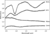 |
Fig. 1 Clones of the VIS-NIR spectra for four asteroids, vertically shifted for clarity. |
2 Data
2.1 Simulating photometry from spectra
We used the collection of about 6000 spectra of Mahlke et al. (2022). We trimmed this dataset to 770 spectra of 596 unique asteroids that cover both VIS and NIR wavelength ranges. We further filtered these spectra to only contain the taxonomic types from the Bus-DeMeo taxonomy, resulting in 754 spectra. Lastly, we removed types with only one object, with the resulting set consisting of 752 objects. This limitation is necessary to test taxonomic predictions on the same dataset for all surveys, thus allowing for a direct comparison of their efficiency.
We then generated clones of these VIS-NIR spectra, increasing the sample size by a factor of ten. Cloning and sampling has been a common practice to increase the sample size for machine learning algorithms (Cellino et al. 2020; Penttilä et al. 2021). This data augmentation simulates the variability of spectra in spectral slope, band contrast, and random noise, due to the intrinsic variability of surfaces (Vernazza et al. 2016; Devogèle et al. 2019; Binzel et al. 2019) or observing and geometry effects (Sanchez et al. 2012; Marsset et al. 2020). We changed the spectral slope and contrast, and added point-to-point noise, using the random Gaussian distribution for the standard deviation 4.2% micron−1 (Marsset et al. 2020), 5%, and 0.01, respectively (Fig. 1). For comparison, the best spectro-photometric measurements originating from all-sky surveys have an error on the order of 0.03 mag. These are conservative values, corresponding to high-quality data: poorly corrected telluric absorptions or differential atmospheric refraction could affect spectra. However, we aim here to characterize suites of filters, so we chose to base our analysis on simulated data reflective of the high standards of current asteroid spectroscopic surveys.
In Table 1 we report the final number of cloned spectra per taxonomic type used in this study. We thus used a sample of 7520 spectra to generate asteroid reflectances. The breakdown of the input spectra into Bus-DeMeo taxonomic types is presented in Table 1. We have divided the data into additional, more general classes (first column in Table 1). That is, all the Bus-DeMeo S subtypes have been merged into a general S class, and all the X subtypes into an X class. Types from the Bus-DeMeo C complex have been split into C and Ch general classes. The later contains the Cgh and Ch types which contain water absorption bands and thus were treated as a separate class. The remaining classes are as in Bus-DeMeo taxonomy. We considered two classification tasks: the Bus-DeMeo types (type prediction) and the more general classes (class prediction) as shown in Table 1.
For each survey presented in the next section, we computed – for each spectrum – fluxes and then reflectances in the survey's filters using the Spectral-Kit for Asteroids (ska1) Python module. This module uses the Spanish Virtual Observatory (SVO) filter profile service to retrieve filter transmission curves (Rodrigo et al. 2012; Rodrigo & Solano 2020). This process is illustrated in Fig. 2. We skipped filters that were not covered by the asteroids' spectral range (e.g., u and v of the SkyMapper survey). We did not simulate the uncertainties, such as those arising from single point photometric uncertainties, rotation, and the cadence of the surveys. Therefore, the computed predictability rates represent the expected top performance of the surveys. The resulting normalized (to one at 0.55 µm) reflectances were used as input for the classification algorithms. An example of the mean values and standard deviations of cloned spectra for a single asteroid – (5) Astraea – for the LSST and VISTA filters are presented in Table 2, and Fig. A.1 contains mean spectra and standard deviations of the clones divided by the taxonomic type.
We note that for a single original spectrum, these values are representative of an object, and higher variability is present in the collection of input data for the entire type containing spectra of a larger number of objects (see Fig. A.1). The influence of the cloning technique on our results is discussed in Sect. 4.
Number of clone spectra per taxonomic class (we grouped subclasses of the Bus-DeMeo taxonomic scheme together) and the Bus-DeMeo type.
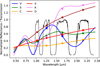 |
Fig. 2 Transmission curves of the VISTA survey Y, J, H, and Ks filters (black lines) against the selected taxonomic types from the Bus-DeMeo taxonomy vertically shifted for illustrative purposes (color lines). The fluxes computed for the VISTA filters are indicated with the filled circles. |
Mean values and standard deviations of LSST and VISTA filters for (5) Astraea.
2.2 Simulated surveys
Based on the spectra above, we simulated fluxes for each major survey for which asteroid color data have been reported or are planned to be obtained in the near future. Most of these surveys focus on other astronomical objects rather than asteroids. They are thus not optimized to detect moving sources nor to discriminate among asteroid taxonomic classes. However, the filters used by those surveys cover several main spectral features of asteroids (Fig. 3). Below we briefly describe each survey considered in this work.
The Sloan Digital Sky Survey (SDSS) was a survey conducted from 1998 to 2009 dedicated to studying the geometry of the Universe (York et al. 2000; Kent 1994). The survey used a 2.5-m wide-angle optical telescope at Apache Point Observatory in New Mexico, United States (Gunn et al. 2006). During its 10 years of operations, it observed a few hundred thousand asteroids (Ivezic et al. 2001) in the u, g, r, i, and z bands (Fukugita et al. 1996). Recently Sergeyev et al. (2021) extracted additional asteroid photometry from the survey for over 350 000 objects.
The SkyMapper Southern Survey (SMSS) is an ongoing survey of the whole southern sky (Wolf et al. 2018). It is being conducted with SkyMapper, a 1.3-m telescope located at Siding Spring Observatory, Coonabarabran, NSW, Australia, it was commissioned in 2007, and is operating in the u, v, g, r, i, and z bands (Keller et al. 2007). Recently, Sergeyev et al. (2022) extracted colors for over 200000 asteroids from the survey's second data release (Onken et al. 2019).
The Legacy Survey of Space and Time (LSST) will be conducted by the Vera C. Rubin observatory, which is currently under construction in Chile. It is expected to be in full scientific operation at the start of 2023. It is expected to discover and characterize more than 5 million asteroids over its ten-year survey lifetime (Jones et al. 2015). The LSST camera covers the spectral range of 0.3-1 µm. The current LSST filter complement (u, g, r, i, z, and y) is modeled after the SDSS system (Olivier et al. 2012).
The ESA Euclid mission. It is a space observatory designed to study the dark universe (Laureijs et al. 2012). It is currently expected to launch in early 2023. Its wide survey will cover 15000 deg2 down to VAB ~ 24.5. It is anticipated to observe and characterize 150000 (mostly in the main belt, Carry 2018) asteroids in VISE, YE, JE, and HE bands (Cropper et al. 2014; Maciaszek et al. 2014; Euclid Collaboration 2022), half of them being potential discoveries, especially at high inclinations (such as Kuiper-belt objects) in the northern hemisphere not covered by LSST (Carry 2018).
The Panoramic Survey Telescope And Rapid Response System (PanSTARRS) is an ongoing two-telescope (PS1 and PS2) survey located at Haleakala Observatory, Hawaii, US (Hodapp et al. 2004a). It is dedicated to moving and variable objects such as near-Earth asteroids. PanSTARRS surveys the asteroids gold spots such the ecliptic, opposition, and low solar-elongation regions (Jedicke et al. 2006). PanSTARRS is equipped with a large number of filters (g, r, w, i, z, and y and open, Hodapp et al. 2004b). Photometric measurements for asteroids from PanSTARRS are regularly submitted to the MPC.
The Visible and Infrared Survey telescope for Astronomy (VISTA) is a 4.1-m telescope located at ESO Paranal Observatory (Emerson & Sutherland 2002). It is mapping the southern sky in Y, J, H, and Ks filters to study the nature of dark matter and dark energy. Popescu et al. (2016) and Popescu et al. (2018) extracted photometry for about 53 500 asteroids with 350000 measurements from the survey and performed a taxonomical classification of those objects.
The Two Micron All-Sky Survey (2MASS) was a survey performed in the years 1997–2001 at the 1.3 m telescopes at Mt. Hopkins and CTIO, Chile (Skrutskie et al. 2006). The survey collected data in the J, H, and Ks to map the three-dimensional distribution of galaxies in the nearby universe (Huchra et al. 2012). The survey collected data for a few thousand asteroids (Sykes et al. 2000).
The Gaia mission. It is an ongoing ESA space mission launched in 2013 and is scanning the entire sky (Prusti et al. 2016). The main goal of the mission is to create a three-dimensional map of the Milky Way; however, it also has dedicated pipelines to study various objects, including asteroids (Tanga & Mignard 2012). The mission will obtain low-resolution spectra for about 100 000 asteroids (Delbo et al. 2012).
The Javalambre Photometric Local Universe Survey (J-PLUS) is dedicated to stellar astrophysics. It uses the JAST/T80 telescope (Javalambre, Spain) equipped with a set of 12 broadband, intermediate-band, and narrowband optical filters at key stellar spectral features for stellar astrophysics. Morate et al. (2021) have provided the first catalog of asteroid colors obtained from the survey for 3122 minor bodies.
The Deep European Near-Infrared Southern Sky Survey (DENIS) survey started in 1995 and was performed at the ESO 1-meter telescope at La Silla, k Chile (Epchtein et al. 1994). The observations were taken at I, J, and K passbands to study extragalactic sources. Baudrand et al. (2004) recovered the color data for 1233 asteroids. Most of them were measured once and some were measured twice in each filter, resulting in 1385 measurements all together.
The AAVSO Photometric All-Sky Survey (APASS) is an all-sky photometric survey providing measurements in eight filters: Johnson B and V, and Sloan u, g, r, i, z, and Z (Henden et al. 2009). The latest data release (10) contains photometry for 128 million objects in about 99% of the sky (Levine 2017). There are some ongoing efforts to extract asteroid colors from the survey (Levine et al. 2019).
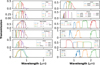 |
Fig. 3 Comparison of filter transmission curves (the filter, instrument, and atmosphere for ground-based surveys and the filter and instrument for space-based surveys) for the different surveys from Sect. 2.2. Transmission curves for J-PLUS are split into two figures for visibility. |
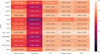 |
Fig. 4 Balanced accuracy for the prediction of classes per survey. |
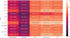 |
Fig. 5 Balanced accuracy for the prediction of types per survey. |
3 Methods and evaluation metrics
We made use of several machine learning classification methods implemented in the Python scikit-learn package (Pedregosa et al. 2011). Those methods have been described in more detail in our recent work (Klimczak et al. 2021), thus they are only briefly summarized below. The descriptions below also list parameter variations, which were used to parameterize each method, with up to tensets of parameters preselected per method.
Multinomial logistic regression (Hastie et al. 2009) estimates the probability of a sample belonging to each class using the soft-max function of a linear combination of input parameters. The weights for each parameter are trained during the learning stage by minimizing the cross-entropy between the empirical class label distribution and the model distribution. For our study, this method was parametrized by inverse regularization strength (values from five to 60) and a regularization norm of either L1(∥w∥1) or  , where w are the weights' vectors.
Naive Bayes (Hastie et al. 2009) uses Bayes theorem to estimate conditional probabilities of each class given the input data and prior probability density function. The algorithm assumes conditional independence between the features. Prior probabilities are calculated from input data, and a Gaussian function is used to model the distribution of features. The variance smoothing parameter was selected between 1e − 10 and 1e − 6 for the purposes of our experiments.
Support vector machines (SVMs) (Hastie et al. 2009) divides the feature space with hyperplanes into regions such that each region corresponds to a single class. Those hyperplanes are obtained in the training phase by maximizing the margin on the data, which is the distance from the nearest sample to the hyperplane. The kernel selected for the experiments was either a radial basis function (RBF) or a linear kernel, regularization ranged from six to 24, gamma automatic (only for the RBF kernel), or scaled.
Gradient boosting (Hastie et al. 2009) combines several learning methods. The methods are added sequentially to the ensemble by minimizing the gradient of the loss function (cross-entropy in this case) so that each new learner improves the performance of the previous model. The number of trees in the experiments ranged from 50 to 500 with the maximum tree depth in between three and 15. The subsampling parameter was either 0.75 or 1, and the learning rate value ranged from 0.01 to 0.1.
MultiLayer Perceptron (MLP) (Goodfellow et al. 2016) – we used a feed-forward artificial neural network with either two or three layers of perceptrons, each with 32 or 64 neurons, followed by a softmax function to obtain the probabilities. Cross-entropy was minimized during the learning phase. The learning rate was selected in between 0.01 and 0.1, and the choice of optimizer was either stochastic gradient descent or Adam.
We performed five runs of five-fold cross-validation for each method to compensate for the randomness of data splitting. In each fold, the parameters of each algorithm were optimized based on the random selection of four-fifths of the data and then evaluated for the remaining fifth of the dataset. Four-fifths of the data were further split into train and validation sets to select the best parameter combination. The optimization of parameters was performed by training up to ten models with different parameters on the subset of data and assessing the performance on the validation split. The parameter combination with the best score (balanced accuracy) was selected and used on the test split (the aforementioned fifth of the data). The result on the test split were recorded. Finally, we report average scores and standard deviations for each algorithm performed by the model with the best parameter combination on the test split. We note that for each method and each survey, we trained up to 500 models (two tasks × tfive runs × five-fold cross-validation × ten parameter combinations). Altogether, this results in 27 500 models (500 models × 11 surveys × five methods) trained in this work. This required significant computing time and processing power. As a result of the size of the dataset, as well as the amount of models that needed to be trained due to the experimental setup, the computing time reached up to 12 h per survey performed on a CPU.
Following Klimczak et al. (2021), we report several evaluation metrics: prediction accuracy (Acc), balanced prediction accuracy (BAcc), F1 measure, and the Matthews correlation coefficient (MCC):

where k is the number of classes, N is the total number of all samples, TPi ("true positives") is the number of correctly classified objects from class i, FPi ("false positives") is the number of objects incorrectly classified as class i, and FNi ("false negatives") is the number of incorrectly classified objects from class i. The MCC measure is known to work well in unbalanced problems. More details about these metrics can be found in Klimczak et al. (2021). Prediction accuracy is used due to its direct interpretability, whereas the balanced accuracy, F1 score, and MCC are known for their robustness against class imbalance, which is the case of this work (Kelleher et al. 2015).
We compliment the aforementioned metrics with confusion matrices for the best performing model and survey (Figs. 6 and 7). These matrices are useful for identifying the classes that were the hardest for the model to predict, and therefore caused the most wrong predictions. In a confusion matrix, the ith row and the jth column (i, j = 1,…, k, k denoting the number of classes) is the number of objects from class i that were predicted to belong to class j.
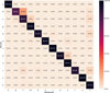 |
Fig. 6 Confusion matrix for the prediction of classes on LSST+VISTA data using a MLP. |
4 Results and discussion
We have performed a taxonomic classification using five different machine learning methods for 11 of the largest surveys relevant to asteroid science. In Figs. B.1–B.4 we report the evaluation metrics (prediction accuracy, balanced accuracy, F1, and MCC, respectively) for all the surveys and methods used in the task of predicting the general taxonomic class (as in Table 1). In Tables B.3–B.6 we show the same metrics, but for the prediction of asteroid Bus-DeMeo types. Colors indicate the highest and lowest scores. Generally, the results are consistent across the different evaluation metrics. Therefore, in what follows we focus on reporting a balanced accuracy, which is one of the most common metrics.
Overall, we achieved a 73–96% balanced accuracy for the most efficient methods in class classification and a 75–90% balanced accuracy for the two most efficient methods in type prediction for the different surveys (with the exception of Gaia). It should be noted that the Bus-DeMeo types were defined using somewhat arbitrary linear borders, thus some machine learning methods could result in poor predictability. Particularly, naive Bayes resulted in low prediction scores. This is due to two factors, first, the assumption of uncorrelated features which is not realistic and, second, the assumption of a Gaussian distribution of parameters in classes.
Sergeyev et al. (2021) and Sergeyev et al. (2022) used a decision tree to assign taxonomic types based on colors from SDSS and SkyMapper and achieved about a 30% success ratio. Penttilä et al. (2021) reported an 86% unbalanced prediction accuracy for classifying Gaia-like asteroid spectra using a neural network. That study used dense VIS spectra, yet we achieve an almost identical 85% unbalanced accuracy for the Euclid survey, despite fewer measurements available. This suggest that there might be an over-abundance of parameters, and there is not a need for dense spectra to achieve a similar prediction rate. Indeed Klimczak et al. (2021) show that the top five and top six features contribute to 93 and 81% of balanced accuracy of complex and type classification, respectively.
The high success ratios in our study could also be due to the conservative bounds in cloning of the original spectra as compared to a larger variation of the simulated spectra in Penttilä et al. (2021). Therefore, our success rates, despite being internally consistent, are not directly comparable with Penttilä et al. (2021).
To assess the usefulness of the clones even further, we performed an additional experiment, where for each object we only selected one clone. This reduced our dataset to 579 samples. Spread across 12 classes and 21 types, the quantity of samples per taxonomic type ranged from four to 169. In this way, we wanted to quantify what scores the models could achieve if we did not use the clones. This experiment was only performed for combined surveys LSST and VISTA, a dataset that yielded the best results in our experiments. The results for the prediction of classes (Table C.1) remained at a relatively high level (74–78% balanced accuracy), falling 20% behind on balanced accuracy compared to the full dataset. What is worth noting is that there is not such a big difference in scores between simpler and more complex models. That is most likely due to the small size of the training data, which was not sufficient enough to train a MLP or gradient boosting. Those models normally operate on much larger volumes of data.
These results are consistent with Klimczak et al. (2021) who reported an ~74–80% balanced accuracy for predicting asteroid types based on the full spectral range for the best performing methods. The training dataset for that study contained spectra for 504 objects split into 12 taxonomic types. Thus the models in Klimczak et al. (2021) were trained on a size-comparable spectral dataset, separated into similar number of types, but on a larger number of features. Interestingly, the top five spectral features (comparable to the number of filters per survey in this study) contributed to the majority of balanced accuracy. Slight differences in the balanced accuracy as compared to Klimczak et al. (2021) might be due to a nonidentical division into types, a larger number of features, and sample size.
For the prediction of taxonomic types (Table C.2), the results are 35% less than for the full dataset. The lower dataset size and higher number of types significantly impacted the predictability power of the models. Again, the results across models do not differ as drastically as they do in the case of the full data.
We conclude that the cloning technique may have impacted the predictability scores, while the sample size and number of predicted classes also play an important role. The number of features beyond the top few has a smaller impact on the resulting balanced accuracy. We highlight that despite the possible estimation of the overall predictability scores, our results are internally consistent.
In the taxonomic class prediction task, three methods (SVM, gradient boosting, and MPL) turned out to be the most efficient, independent of the survey. In taxonomic-type predictions, gradient boosting and MPL performed the best across all surveys. Naive Bayes was the worst performing algorithm in both tasks. Naive Bayes assumes an independence between the features. Generally, the scores for predicting the taxonomic class are higher than that for predicting asteroid types. This is expected, as the general classes contain multiple types and are thus easier to predict.
Despite having just a few filters, the VISTA survey (four broadband filters) and Euclid mission (three broadband filters) were the best-performing surveys in both class and type prediction tasks. In the prediction of the taxonomic class, both surveys achieved around a 93% balanced prediction accuracy in the gradient boosting method. For the type prediction, both reached about 85% BAcc. A higher balanced accuracy was only achieved for combined surveys (e.g.,a 90 and 96% balanced accuracy for a combination of LSST and VISTA data in type and in complex prediction, respectively). This is not surprising as the Bus-DeMeo taxonomy is based on combined VIS and NIR spectra, thus classifications made using only a subset of the wavelengths should perform poorer.
Though the gradient boosting was the most efficient method for Euclid and VISTA surveys, these surveys outperformed all the others independent of the method and metric used. One exception is naive Bayes, for which the balanced accuracy of Euclid is on the level of other surveys and the VISTA and 2MASS surveys performed the best in complex prediction. The broad VISTA and Euclid surveys' filters covered the 1 and 2 µm olivine and pyroxene absorption bands well, which are the most pronounced spectral features. Owing to the well-matching wavelength coverage, VISTA and Euclid performed the best in our study out of single survey.
Having complementary data in wavelengths, for example for LSST (VIS) and VISTA (NIR), can further boost the prediction score. For the combination of LSST and VISTA data, we obtain about a 96% balanced accuracy for predicting the taxonomic class and around 90% for predicting taxonomic types for the most efficient methods. In Figs. 6 and 7, we show confusion matrices for the prediction of taxonomic classes and types, respectively. Values on the diagonal represent correct classifications, whereas the values off the diagonal are misclassifications. As expected, some taxonomic types are easier to predict than others. The unique and distinct V-type objects are never misclassified, whereas for example types within the S, C, and X complexes are sometimes misclassified. This is a natural consequence of the fact that the spectra of asteroids in the complexes are rather similar and thus difficult to separate by machine learning algorithms. Some misclassification is also visible between the C and X complexes which often have similar spectra differing, just in the spectral slope or albedo.
The worst performing survey in our experiment is the Gaia mission, for which we only considered the G, Grp, and Gbp magnitudes, that were available from Gaia at the time of our experiments. When the mission obtains asteroid spectra in the visible wavelengths (from 0.325 to 1.1 µm) for 100 000 objects Mignard et al. (2007), the performance may change significantly. Linking asteroid spectra to the Bus-DeMeo taxonomy was performed earlier by Penttilä et al. (2021), who achieved an 86% unbalanced prediction accuracy for 11 taxonomic types considered. In this work we focus on Gaia spectro-photometry, which may be useful for faint sources for which full spectroscopy is not possible. With just the three filters, Gaia scoredan 81% balanced prediction accuracy for MLP, 77% for SVM, and 73% for gradient boosting as a prediction of the asteroid complex. For the taxonomic-type prediction, it reached a 63% balanced accuracy for MLP, 57% for gradient boosting, and 61% for SVM. The lowest score for Gaia was for naive Bayes. Moving to MLP, that score improved over 2.5 times. Clearly selecting the right prediction algorithm can optimize the science output. This seems even more critical for surveys with fewer filters not optimized for asteroid taxonomy.
Other surveys, conducted in the VIS wavelengths (LSST, PANSTARSS, SDSS, and SkyMapper) have a similar wavelength coverage and filter set, thus all perform similarly, on the level of an 80–90% balanced accuracy for the class prediction for gradient boosting and MLP. For the type prediction, they achieve a 70–80% balanced accuracy for the two best methods. Out of the visible surveys, LSST and PanSTARRS perform slightly better than the rest in both tasks. This is likely due to the higher number of filters. However, the improvement in performance is minuscule (on the order of 3–4%).
The surveys performed in the NIR considered in this work are VISTA, DENIS, Euclid, and 2MASS. All of those surveys have broader and fewer filters than the VIS surveys. Despite that, as discussed earlier, VISTA and Euclid are the best scoring surveys in this work and the remaining NIR surveys performed very similarly to the VIS surveys. They achieve an 80-90% balanced accuracy in the class prediction and a 70–80% balanced accuracy in the type prediction. This due to the fact that many of the taxonomic types differ more in NIR wavelengths.
Moskovitz et al. (2008) used SDSS colors to identify V-type candidates and reported a 90% success rate based on spectral observations. Similarly, high observational success rates for confirming V-type asteroids were also found by other studies (Solontoi et al. 2012; Oszkiewicz et al. 2014). The V types are, however, the easiest to predict due to characteristic spectra with strong absorption bands. In our work, the V-type prediction reaches even a 100% accuracy for MLP and the gradient boosting. DeMeo et al. (2019) report a 33% observational success ratio for A-type candidates selected based on SDSS colors and DeMeo et al. (2014) report up to 40% for multiply observed D-type candidates. These rates are much lower than what we observe. We note that based on visible filters, only the A types might be easily confused with the S types and D types with X-complex objects. Furthermore, the success ratios indicated by us represent the top possible prediction rates. Our simulation did not include random or systematic photometric uncertainties and assumed that spectro-photometry gives exact measurements corrected for rotational variation. In reality, correction for rotational brightness modulation is not possible for many asteroids as rotation periods and light-curve amplitudes are simply not known for many of the objects. Furthermore, the convoluted fluxes in our work were computed from spectra normalized at 0.55 Surveys produce multifilter photometry and typically do not cover 0.55 µm – maximum of the Solar irradiance. Thus one of the filters has to be used for normalization. This could result in lower success scores in reality.
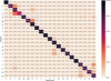 |
Fig. 7 Confusion matrix for the prediction of taxonomic types on LSST+VISTA data using a MLP. |
5 Conclusions
We performed a number of experiments to investigate which machine learning methods are best suitable for predicting asteroid types and more general classes. We simulated fluxes for 11 different space- and ground-based surveys that are commonly used for various taxonomic studies in planetary science.
Out of the five machine learning methods, gradient boosting and MLPs performed the best, followed by SVM in both tasks of classifying asteroids into types and classes. The worst performing method was Naive Bayes, which achieved scores about 2.5 times worse than the best methods in this study. Clearly, selecting the right machine learning algorithm for predicting asteroid types can boost the science output of each survey.
Despite having just a few broadband filters, the best performing surveys were Euclid and VISTA, reaching 85 and 93% of balanced accuracy in type and class prediction, respectively. Those surveys cover the 1- ans 2-µm olivine and pyroxene absorption bands well – the most apparent features of asteroid spectra. In order to maximize the science output for Solar System science, the right choice of filters covering the most important spectral features has to be made for future surveys targeting asteroids.
Acknowledgments
This work has been supported by the grant No. 2017/25/B/ST9/00740 from the National Science Centre, Poland. This research has made use of the SVO Filter Profile Service (http://svo2.cab.inta- csic.es/theory/fps/) supported from the Spanish MINECO through grant AYA2017-84089.
Appendix A Variability of the clones
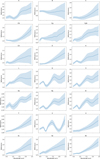 |
Fig. A.1 Mean values and standard deviations of spectra per taxonomic type. |
Appendix B Accuracy, F1, and MCC scores
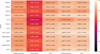 |
Fig. B.1 Accuracy for the prediction of classes per survey. |
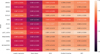 |
Fig. B.2 F1 for the prediction of classes per survey. |
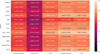 |
Fig. B.3 Accuracy for the prediction of types per survey. |
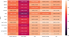 |
Fig. B.4 MCC for the prediction of classes per survey. |
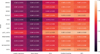 |
Fig. B.5 F1 for the prediction of types per survey. |
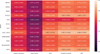 |
Fig. B.6 MCC for the prediction of types per survey. |
Appendix C The results on reduced data for LSST+VISTA
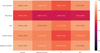 |
Fig. C.1 Results for the prediction of class on the reduced dataset with LSST+VISTA data. |
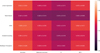 |
Fig. C.2 Results for the prediction of taxonomic types on the reduced dataset with LSST+VISTA data. |
References
- Baudrand, A., Bec-Borsenberger, A., & Borsenberger, J. 2004, A&A, 423, 381 [NASA ADS] [CrossRef] [EDP Sciences] [Google Scholar]
- Binzel, R., DeMeo, F., Turtelboom, E., et al. 2019, Icarus, 324, 41 [NASA ADS] [CrossRef] [Google Scholar]
- Bus, S. J., & Binzel, R. P. 2002, Icarus, 158, 146 [Google Scholar]
- Carry, B. 2018, A&A, 609, A113 [NASA ADS] [CrossRef] [EDP Sciences] [Google Scholar]
- Carry, B., Solano, E., Eggl, S., & DeMeo, F. E. 2016, Icarus, 268, 340 [CrossRef] [Google Scholar]
- Carvano, J., Hasselmann, P., Lazzaro, D., & Mothé-Diniz, T. 2010, A&A, 510, A43 [NASA ADS] [CrossRef] [EDP Sciences] [Google Scholar]
- Cellino, A., Bendjoya, P., Delbo, M., et al. 2020, A&A, 642, A80 [NASA ADS] [CrossRef] [EDP Sciences] [Google Scholar]
- Colazo, M., Alvarez-Candal, A., & Duffard, R. 2022, A&A, 666, A77 [NASA ADS] [CrossRef] [EDP Sciences] [Google Scholar]
- Cropper, M., Pottinger, S., Niemi, S. M., et al. 2014, SPIE Conf. Ser., 9143, 91430J [NASA ADS] [Google Scholar]
- Delbo, M., Gayon-Markt, J., Busso, G., et al. 2012, Planet. Space Sci., 73, 86 [CrossRef] [Google Scholar]
- DeMeo, F., & Carry, B. 2013, Icarus, 226, 723 [NASA ADS] [CrossRef] [Google Scholar]
- DeMeo, F. E., & Carry, B. 2014, Nature, 505, 629 [NASA ADS] [CrossRef] [Google Scholar]
- DeMeo, F. E., Binzel, R. P., Slivan, S. M., & Bus, S. J. 2009, Icarus, 202, 160 [Google Scholar]
- DeMeo, F. E., Binzel, R. P., Carry, B., Polishook, D., & Moskovitz, N. A. 2014, Icarus, 229, 392 [NASA ADS] [CrossRef] [Google Scholar]
- DeMeo, F. E., Polishook, D., Carry, B., et al. 2019, Icarus, 322, 13 [CrossRef] [Google Scholar]
- Devogèle, M., Moskovitz, N., Thirouin, A., et al. 2019, AJ, 158, 196 [CrossRef] [Google Scholar]
- Emerson, J. P., & Sutherland, W. 2002, Int. Soc. Opt. Photonics, 4836, 35 [NASA ADS] [Google Scholar]
- Epchtein, N., De Batz, B., Copet, E., et al. 1994, in Science with Astronomical Near-Infrared Sky Surveys (Berlin: Springer), 3 [CrossRef] [Google Scholar]
- Erasmus, N., McNeill, A., Mommert, M., et al. 2019, ApJS, 242, 15 [NASA ADS] [CrossRef] [Google Scholar]
- Erasmus, N., Navarro-Meza, S., McNeill, A., et al. 2020, ApJS, 247, 13 [CrossRef] [Google Scholar]
- Euclid Collaboration (Schirmer, M., et al.) 2022, A&A, 662, A92 [NASA ADS] [CrossRef] [EDP Sciences] [Google Scholar]
- Fukugita, M., Ichikawa, T., Gunn, J., et al. 1996, AJ, 111, 1748 [NASA ADS] [CrossRef] [Google Scholar]
- Gaia Collaboration (Galluccio, L., et al.) 2022, A&A, in press https://doi.org/10.1051/0004-6361/202243791 [Google Scholar]
- Goodfellow, I. J., Bengio, Y., & Courville, A. 2016, Deep Learning (Cambridge, MA, USA: MIT Press) [Google Scholar]
- Gunn, J. E., Siegmund, W. A., Mannery, E. J., et al. 2006, AJ, 131, 2332 [NASA ADS] [CrossRef] [Google Scholar]
- Hastie, T., Tibshirani, R., & Friedman, J. 2009, The Elements of Statistical Learning: Data Mining, Inference and Prediction, 2nd edn. (Berlin: Springer) [Google Scholar]
- Henden, A. A., Welch, D., Terrell, D., & Levine, S. 2009, AAS Meeting Abstracts, 214, 407 [Google Scholar]
- Hodapp, K., Kaiser, N., Aussel, H., et al. 2004a, Astron. Nachr. Astron. Notes, 325, 636 [NASA ADS] [CrossRef] [Google Scholar]
- Hodapp, K. W., Siegmund, W. A., Kaiser, N., et al. 2004b, Int. Soc. Opt. Photonics, 5489, 667 [Google Scholar]
- Huchra, J. P., Macri, L. M., Masters, K. L., et al. 2012, ApJS, 199, 26 [Google Scholar]
- Ivezic, Ž., Tabachnik, S., Rafikov, R., et al. 2001, AJ, 122, 2749 [NASA ADS] [CrossRef] [Google Scholar]
- Ivezic, Ž., Lupton, R. H., Juric, M., et al. 2002, AJ, 124, 2943 [CrossRef] [Google Scholar]
- Ivezic, Ž., Connolly, A. J., VanderPlas, J. T., & Gray, A. 2019, Statistics, Data Mining, and Machine Learning in Astronomy: A Practical Python Guide for the Analysis of Survey Data (Princeton: Princeton University Press) [Google Scholar]
- Jedicke, R., Magnier, E., Kaiser, N., & Chambers, K. 2006, Proc. Int. Astron. Union, 2, 341 [CrossRef] [Google Scholar]
- Jones, R. L., Juric, M., & Ivezic, Ž. 2015, Proc. Int. Astron. Union, 10, 282 [CrossRef] [Google Scholar]
- Kelleher, J. D., Namee, B. M., & D’Arcy, A. 2015, Fundamentals of Machine Learning for Predictive Data Analytics: Algorithms, Worked Examples, and Case Studies (Cambridge: MIT Press) [Google Scholar]
- Keller, S. C., Schmidt, B. P., Bessell, M. S., et al. 2007, PASA, 24, 1 [NASA ADS] [CrossRef] [Google Scholar]
- Kent, S. M. 1994, Astrophys. Space Sci., 217, 27 [NASA ADS] [CrossRef] [Google Scholar]
- Klimczak, H., Kotłowski, W., Oszkiewicz, D. A., et al. 2021, Front. Astron. Space Sci., 216 [Google Scholar]
- Laureijs, R., Gondoin, P., Duvet, L., et al. 2012, SPIE, 8442, 84420T [NASA ADS] [Google Scholar]
- Levine, S. 2017, J. Am. Assoc. Variab. Star Observers, 45, 127 [NASA ADS] [Google Scholar]
- Levine, S., Henden, A., Terrell, D., Welch, D., & Kloppenborg, B. 2019, J. Am. Assoc. Variab. Star Observers, 47, 132 [NASA ADS] [Google Scholar]
- Licandro, J., Popescu, M., Morate, D., & de León, J. 2017, A&A, 600, A126 [NASA ADS] [CrossRef] [EDP Sciences] [Google Scholar]
- Maciaszek, T., Ealet, A., Jahnke, K., et al. 2014, SPIE Conf. Ser., 9143, 91430K [NASA ADS] [Google Scholar]
- Mahlke, M., Carry, B., & Mattei, P.-A. 2022, A&A, 665, A26 [NASA ADS] [CrossRef] [EDP Sciences] [Google Scholar]
- Mansour, J.-A., Popescu, M., de León, J., & Licandro, J. 2020, MNRAS, 491, 5966 [NASA ADS] [CrossRef] [Google Scholar]
- Marsset, M., DeMeo, F. E., Binzel, R. P., et al. 2020, ApJS, 247, 73 [NASA ADS] [CrossRef] [Google Scholar]
- Mignard, F., Cellino, A., Muinonen, K., et al. 2007, Earth Moon Planets, 101, 97 [Google Scholar]
- Mommert, M., Trilling, D., Borth, D., et al. 2016, AJ, 151, 98 [NASA ADS] [CrossRef] [Google Scholar]
- Morate, D., Carvano, J. M., Alvarez-Candal, A., et al. 2021, A&A, 655, A47 [NASA ADS] [CrossRef] [EDP Sciences] [Google Scholar]
- Moskovitz, N. A., Jedicke, R., Gaidos, E., et al. 2008, Icarus, 198, 77 [NASA ADS] [CrossRef] [Google Scholar]
- Nesvorny, D., Jedicke, R., Whiteley, R. J., & Ivezic, Ž. 2005, Icarus, 173, 132 [CrossRef] [Google Scholar]
- Olivier, S. S., Riot, V. J., Gilmore, D. K., et al. 2012, SPIE, 8446, 84466B [NASA ADS] [Google Scholar]
- Onken, C. A., Wolf, C., Bessell, M. S., et al. 2019, PASA, 36, e033 [Google Scholar]
- Oszkiewicz, D., Kwiatkowski, T., Tomov, T., et al. 2014, A&A, 572, A29 [NASA ADS] [CrossRef] [EDP Sciences] [Google Scholar]
- Parker, A., Ivezic, Ž., Juric, M., et al. 2008, Icarus, 198, 138 [NASA ADS] [CrossRef] [Google Scholar]
- Pedregosa, F., Varoquaux, G., Gramfort, A., et al. 2011, J. Mach. Learn. Res., 12, 2825 [Google Scholar]
- Penttilä, A., Hietala, H., Muinonen, K., et al. 2021, A&A, 649, A46 [NASA ADS] [CrossRef] [EDP Sciences] [Google Scholar]
- Popescu, M., Birlan, M., & Nedelcu, D. 2012, A&A, 544, A130 [NASA ADS] [CrossRef] [EDP Sciences] [Google Scholar]
- Popescu, M., Licandro, J., Morate, D., et al. 2016, A&A, 591, A115 [NASA ADS] [CrossRef] [EDP Sciences] [Google Scholar]
- Popescu, M., Licandro, J., de Leon, J., Morate, D., & Boaca, I. L. 2018, in European Planetary Science Congress, EPSC2018-273 [Google Scholar]
- Prusti, T., De Bruijne, J., Brown, A. G., et al. 2016, A&A, 595, A1 [NASA ADS] [CrossRef] [EDP Sciences] [Google Scholar]
- Rodrigo, C., & Solano, E. 2020, in XIV.0 Scientific Meeting (virtual) of the Spanish Astronomical Society, 182 [Google Scholar]
- Rodrigo, C., Solano, E., & Bayo, A. 2012, SVO Filter Profile Service Version 1.0, IVOA Working Draft 15 October 2012 [Google Scholar]
- Sanchez, J. A., Reddy, V., Nathues, A., et al. 2012, Icarus, 220, 36 [CrossRef] [Google Scholar]
- Sergeyev, A. V., & Carry, B. 2021, A&A, 652, A59 [NASA ADS] [CrossRef] [EDP Sciences] [Google Scholar]
- Sergeyev, A., Carry, B., Onken, C., et al. 2022, A&A, 658, A109 [NASA ADS] [CrossRef] [EDP Sciences] [Google Scholar]
- Skrutskie, M., Cutri, R., Stiening, R., et al. 2006, AJ, 131, 1163 [Google Scholar]
- Solontoi, M. R., Hammergren, M., Gyuk, G., & Puckett, A. 2012, Icarus, 220, 577 [NASA ADS] [CrossRef] [Google Scholar]
- Sykes, M. V., Cutri, R. M., Fowler, J. W., et al. 2000, Icarus, 146, 161 [NASA ADS] [CrossRef] [Google Scholar]
- Tanga, P., & Mignard, F. 2012, Planet. Space Sci., 73, 5 [NASA ADS] [CrossRef] [Google Scholar]
- Tanga, P., Pauwels, T., Mignard, F., et al. 2022, A&A, in press, https://doi.org/10.1051/0004-6361/202243796 [Google Scholar]
- Tholen, D. J. 1989, Asteroids II (Tucson: University of Arizona Press), 1139 [Google Scholar]
- Thomas, C. A., Trilling, D. E., & Rivkin, A. S. 2012, Icarus, 219, 505 [NASA ADS] [CrossRef] [Google Scholar]
- Torppa, J., Granvik, M., Penttilä, A., et al. 2018, Adv. Space Res., 62, 464 [NASA ADS] [CrossRef] [Google Scholar]
- Vernazza, P., Marsset, M., Beck, P., et al. 2016, AJ, 152, 54 [CrossRef] [Google Scholar]
- Wolf, C., Onken, C. A., Luvaul, L. C., et al. 2018, PASA, 35, e010 [Google Scholar]
- York, D. G., Adelman, J., Anderson Jr, J. E., et al. 2000, AJ, 120, 1579 [NASA ADS] [CrossRef] [Google Scholar]
- Zellner, B., Tholen, D., & Tedesco, E. 1985, Icarus, 61, 355 [NASA ADS] [CrossRef] [Google Scholar]
All Tables
Number of clone spectra per taxonomic class (we grouped subclasses of the Bus-DeMeo taxonomic scheme together) and the Bus-DeMeo type.
All Figures
|
Fig. 1 Clones of the VIS-NIR spectra for four asteroids, vertically shifted for clarity. |
| In the text | |
|
Fig. 2 Transmission curves of the VISTA survey Y, J, H, and Ks filters (black lines) against the selected taxonomic types from the Bus-DeMeo taxonomy vertically shifted for illustrative purposes (color lines). The fluxes computed for the VISTA filters are indicated with the filled circles. |
| In the text | |
|
Fig. 3 Comparison of filter transmission curves (the filter, instrument, and atmosphere for ground-based surveys and the filter and instrument for space-based surveys) for the different surveys from Sect. 2.2. Transmission curves for J-PLUS are split into two figures for visibility. |
| In the text | |
|
Fig. 4 Balanced accuracy for the prediction of classes per survey. |
| In the text | |
|
Fig. 5 Balanced accuracy for the prediction of types per survey. |
| In the text | |
|
Fig. 6 Confusion matrix for the prediction of classes on LSST+VISTA data using a MLP. |
| In the text | |
|
Fig. 7 Confusion matrix for the prediction of taxonomic types on LSST+VISTA data using a MLP. |
| In the text | |
|
Fig. A.1 Mean values and standard deviations of spectra per taxonomic type. |
| In the text | |
|
Fig. B.1 Accuracy for the prediction of classes per survey. |
| In the text | |
|
Fig. B.2 F1 for the prediction of classes per survey. |
| In the text | |
|
Fig. B.3 Accuracy for the prediction of types per survey. |
| In the text | |
|
Fig. B.4 MCC for the prediction of classes per survey. |
| In the text | |
|
Fig. B.5 F1 for the prediction of types per survey. |
| In the text | |
|
Fig. B.6 MCC for the prediction of types per survey. |
| In the text | |
|
Fig. C.1 Results for the prediction of class on the reduced dataset with LSST+VISTA data. |
| In the text | |
|
Fig. C.2 Results for the prediction of taxonomic types on the reduced dataset with LSST+VISTA data. |
| In the text | |
Current usage metrics show cumulative count of Article Views (full-text article views including HTML views, PDF and ePub downloads, according to the available data) and Abstracts Views on Vision4Press platform.
Data correspond to usage on the plateform after 2015. The current usage metrics is available 48-96 hours after online publication and is updated daily on week days.
Initial download of the metrics may take a while.