| Issue |
A&A
Volume 677, September 2023
|
|
|---|---|---|
| Article Number | L17 | |
| Number of page(s) | 11 | |
| Section | Letters to the Editor | |
| DOI | https://doi.org/10.1051/0004-6361/202347484 | |
| Published online | 22 September 2023 | |
Letter to the Editor
A high HDO/H2O ratio in the Class I protostar L1551 IRS5⋆
1
Institut de Recherche en Astrophysique et Planétologie (IRAP), Université de Toulouse, UT3-PS, CNRS, CNES, 9 av. du Colonel Roche, 31028 Toulouse Cedex 4, France
e-mail: This email address is being protected from spambots. You need JavaScript enabled to view it.
; This email address is being protected from spambots. You need JavaScript enabled to view it.
2
Konkoly Observatory, Research Centre for Astronomy and Earth Sciences, Eötvös Loránd Research Network (ELKH), Konkoly-Thege Miklós út 15-17, 1121 Budapest, Hungary
3
CSFK, MTA Centre of Excellence, Budapest, Konkoly Thege Miklós út 15-17, 1121 Budapest, Hungary
4
Centre for Star and Planet Formation, Niels Bohr Institute & Natural History Museum of Denmark, University of Copenhagen, Øster Voldgade 5-7, 1350 Copenhagen K, Denmark
5
Max-Planck-Institut für Astronomie, Königstuhl 17, 69117 Heidelberg, Germany
6
Eötvös Loránd University, Department of Astronomy, Pázmány Péter sétány 1/A, 1117 Budapest, Hungary
7
Institute of Astronomy, Department of Physics, National Tsing Hua University, Hsinchu, Taiwan
Received:
17
July
2023
Accepted:
29
August
2023
Abstract
Context. Water is a very abundant molecule in star-forming regions. Its deuterium fractionation provides an important tool for understanding its formation and evolution during the star and planet formation processes. While the HDO/H2O abundance ratio has been determined toward several young Class 0 protostars and comets, the number of studies toward Class I protostars is limited.
Aims. Our aim is to study the water deuteration toward the Class I protostellar binary L1551 IRS5 and to investigate the effect of evolutionary stage and environment on variations in the water D/H ratio.
Methods. Observations were carried out toward L1551 IRS5 using the NOrthern Extended Millimeter Array (NOEMA) interferometer. The HDO 31, 2–22, 1 transition at 225.9 GHz and the H218O 31, 3–22, 0 transition at 203.4 GHz were covered with a spatial resolution of 0.5″× 0.8″, while the HDO 42, 2–42, 3 transition at 143.7 GHz was observed with a resolution of 2.0″ × 2.5″. We constrained the water D/H ratio using both local thermodynamic equilibrium (LTE) and non-LTE models.
Results. The three transitions are detected. The line profiles display two peaks, one at ∼6 km s−1 and one at ∼9 km s−1. We derive an HDO/H2O ratio of (2.1 ± 0.8) × 10−3 for the redshifted component and a lower limit of > 0.3 × 10⁻³ for the blueshifted component. This lower limit is due to the blending of the blueshifted H218O component with redshifted CH3OCH3 emission.
Conclusions. The HDO/H2O ratio in L1551 IRS5 is similar to the values in Class 0 isolated sources and in the disk of the Class I protostar V883 Ori, while it is significantly higher than in the previously studied clustered Class 0 sources and the comets. This result suggests that the chemistry of protostars that belong to molecular clouds with relatively low source densities, such as L1551, share more similarities with the isolated sources than the protostars of very dense clusters. If the HDO/H2O ratios in Class 0 protostars with few sources around are comparable to those found to date in isolated Class 0 objects, it would mean that there is little water reprocessing from the Class 0 to Class I protostellar stage.
Key words: astrochemistry / stars: protostars / stars: formation / ISM: molecules / ISM: individual objects: L1551 IRS5
This work is based on observations carried out under project numbers W18AO and S16AE with the IRAM NOEMA Interferometer. IRAM is supported by INSU/CNRS (France), MPG (Germany), and IGN (Spain).
© The Authors 2023
 Open Access article, published by EDP Sciences, under the terms of the Creative Commons Attribution License (https://creativecommons.org/licenses/by/4.0), which permits unrestricted use, distribution, and reproduction in any medium, provided the original work is properly cited.
This article is published in open access under the Subscribe to Open model. This email address is being protected from spambots. You need JavaScript enabled to view it. to support open access publication.
1. Introduction
Water is one of the most abundant molecules in the interstellar medium. Its role is significant in the star formation process as it cools down the warm regions and boosts the gravitational collapse. It has been detected in multiple environments, such as protostars (e.g., van Dishoeck et al. 2021), protoplanetary disks (e.g., Hogerheijde et al. 2011), comets (e.g., Mumma et al. 1986; Davies et al. 1997), and asteroids (e.g., Rivkin & Emery 2010). Deuteration is extremely sensitive to density and temperature conditions (Ceccarelli et al. 2014), and higher D/H ratios are expected in particular when water forms in cold and dense conditions (e.g., Coutens et al. 2012; Jensen et al. 2019). The comparison of the D/H abundance ratio of the terrestrial oceans (Vienna Standard Mean Ocean Water (VSMOW) ∼ 1.557 × 10⁻⁴, de Laeter et al. 2003) with comets and asteroids (a few 10−4) suggests that these primitive objects could have delivered part of the water found on Earth (e.g., Hartogh et al. 2011; Altwegg et al. 2015; Trigo-Rodríguez et al. 2019). Chemical models of water deuteration in protoplanetary disks also show that the fractionation is not efficient enough to reproduce the terrestrial water D/H ratio without considering an inheritance from the parental molecular cloud (Cleeves et al. 2014). Studying the water deuteration in protostars can consequently help understand the origin of water in disks and planets (Furuya et al. 2016).
During the last decade the water deuterium fractionation ratio1 has been measured in the warm inner regions of several Class 0 protostars, thanks to interferometric observations with the Atacama Large Millimeter/submillimeter Array (ALMA), the Submillimeter Array, and the Plateau de Bure Interferometer (Jørgensen & van Dishoeck 2010; Taquet et al. 2013; Coutens et al. 2014, and references thereafter). In the clustered sources (IRAS 16293−2422, NGC 1333 IRAS2A, IRAS4A−NW, and IRAS4B) the HDO/H2O ratio was found to range between 6 × 10⁻⁴ and 19 × 10−4 (Persson et al. 2013, 2014). However, for the isolated sources (L483, B335, and BHR71−IRS1) Jensen et al. (2019) found a HDO/H2O ratio of (1.7–2.2) × 10−3, which is a factor of ∼2–4 higher than for the clustered sources. This difference was proposed to be the consequence of different durations or temperatures in the prestellar phase (Jensen et al. 2021).
To reconstruct the full history of water during the star formation process and bridge the gap between the Class 0 protostellar stage and the formation of planets, comets, and asteroids, studies of more evolved protostars are needed. Even if the detection of water is usually difficult in such sources (Harsono et al. 2020), there are a few Class I objects in which water can be detected, for example after a strong increase in the accretion rate from the disk onto the protostar (e.g., FUor or EXor sources, Audard et al. 2014; Fischer et al. 2022). Such an event leads to a luminosity burst that warms up the disk and the envelope in which the icy grain mantles can sublimate (Cieza et al. 2016). However, the studies were limited to only two sources. A first study by Codella et al. (2016) showed the detection of HDO toward the EXor-like source SVS13-A with the IRAM 30 m telescope. The presence of high-energy transitions suggests that they come from the warm inner regions even though emission from large-scale shocks cannot be excluded. From the nondetection of the  transition at 203.4 GHz, they estimated a lower limit of the HDO/H2O ratio of ≳10−3. More recently, a HDO/H2O ratio of (2.26 ± 0.63) × 10−3 was obtained with ALMA in the disk of the FUor protostar V883 Ori (Tobin et al. 2023). The similarity of the water deuteration in isolated Class 0 protostars supports the inheritance of water from the envelope to the disk.
Here we report the interferometric determination of the HDO/H2O ratio in another Class I source, L1551 IRS5 (Chen et al. 1995). This protostellar binary, located in the Taurus molecular cloud (d ∼ 155 pc, Zucker et al. 2019), is classified as a FUor-like object by Connelley & Reipurth (2018) based on its near-infrared spectra (Mundt et al. 1985; Carr et al. 1987). The detection of complex organic molecules in its inner regions suggests high-temperature conditions that would be sufficient to thermally desorb the molecules frozen on grains, similarly to hot corinos (Bianchi et al. 2020; Cruz-Sáenz de Miera, in prep.).
2. Observations
Observations of two HDO transitions and one  transition were carried out toward L1551 IRS5 with the Northern Extended Millimeter Array (NOEMA) through the projects W18AO and S16AE (see Table 1). The HDO 31, 2–22, 1 and
  31, 3–22, 0 transitions at 225.9 GHz and 203.4 GHz, respectively, were observed simultaneously in the A configuration on 15 and 17 February 2019 and in the C configuration on 27 February 2019. High spectral resolution windows with channel spacing of 62.5 kHz (i.e., 0.08–0.09 km s−1) were used to cover the two transitions. We resampled the data with a resolution dv of 0.5 km s−1 to increase the signal-to-noise ratio. The HDO 42, 2–42, 3 transition at 143.7 GHz was covered with a poor resolution of 1.95 MHz (i.e., 4 km s−1) in other NOEMA observations carried out on 25 August and 31 August 2016 in the D configuration. All the data were calibrated and imaged using the CLIC and MAPPING packages of the GILDAS2 software. The list of calibrators for each observation is in Table A.1. The continuum was subtracted before the Fourier transform was applied to the line data. The data were imaged with the natural weighting mode. The synthesized beam sizes and rms obtained for each transition are listed in Table 1. The two components, N and S, of L1551 IRS5 are not fully resolved in our observations as they are only separated by 0.36″ (i.e., ∼56 AU, Cruz-Sáenz de Miera et al. 2019).
Detected HDO and  transitions toward the L1551 IRS5 source.
3. Results
In a first step, we visualized the datacubes of the HDO and  lines with the Aladin3 and CASSIS4 softwares (Bonnarel et al. 2000; Glorian et al. 2021). We extracted the spectra at the positions of the northern source (αJ2000 =
  , δJ2000 = +18° 08′04.72″) and the southern source (αJ2000 =
  , δJ2000 = +18° 08′04.359″, Takakuwa et al. 2020). To study variations in the line intensities with the position, the spectra were also extracted for a position between the two sources, at an equal distance from them (
 , δJ2000 = +18° 08′04.550″), that we call M. Because of the asymmetry in emission maps with respect to M, we include a position at a similar distance from N in the opposite direction (
 , δJ2000 = +18° 08′04.890″) called O. A comparison of these spectra is shown in Fig. 1, and their locations are indicated in Fig. 2.
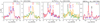 |
Fig. 1. Comparison of the spectra of the water isotopolog transitions. The green, blue, red, and orange solid lines represent the spectra extracted at the position S, M, N, and O, respectively. The dotted lines show velocities of 6.0 km s−1 (blue) and 9.5 km s−1 (red). Considering the synthetic beam sizes and the separation of the N and S components, the extracted spectra are not entirely independent from each other. For the HDO line at 143.7 GHz, the spatial resolution is too low to distinguish O from N and M from S. The x-axis scale is larger for this transition. |
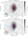 |
Fig. 2. Integrated emission maps of the HDO line at 225.9 GHz (top) and the |

Two velocity components are seen in the line profiles at 203.4 and 225.9 GHz, similarly to Bianchi et al. (2020) and Mercimek et al. (2022) for complex organic molecules. The component at ∼9 km s−1 is brighter at the N and O positions than at the M and S positions. The HDO component at ∼6 km s−1 is slightly brighter at the M position than the N and S positions, while it is less bright at the O position. The high-velocity peak corresponds to the N source or farther to the north, in agreement with Bianchi et al. (2020). The HDO component at 6 km s−1 seems to arise closer to the M position than the S position based on the comparison of the observed line intensities. The double peak created by these two velocity components could then possibly indicate rotation from a disk surrounding the N source. For the HDO line at 143.7 GHz, the spatial resolution is too low (∼2.0–2.5″) compared to the binary separation (0.36″) to observe spectral differences at the four positions (see Fig. 1). The two velocity components are not observed because of the low spectral resolution of the data (4 km s−1).
We used the CASSIS software to check possible blending with other molecules at velocities of both 6 km s−1 and 9 km s−1. The spectroscopic data come from the CDMS and JPL databases (Pickett et al. 1998; Müller et al. 2005). No blending is observed for the component at ∼9 km s−1 either for HDO or  . However, the
  component at ∼6 km s−1 is blended with a CH3OCH3 33, 1, 1–22, 1, 1 line emitted at ∼9 km s−1. A faint line of CH3OCHO 66, 0–55, 0 (emission at 9 km s−1) is observed in the wing of the HDO transition at 225.9 GHz. The HDO line at 143.7 GHz does not seem to be affected by blending.
Integrated emission maps of the HDO 225.9 GHz and  203.4 GHz lines are shown in Fig. 2. The water emission is compact (less than 70 AU in diameter), as also seen for complex organic molecules (Bianchi et al. 2020). As expected, the HDO component at 9 km s−1 (in red) peaks close to the N position, while the one at 6 km s−1 (in blue) peaks closer to the M position. A similar distribution is seen for the
  component at 9 km s−1. However, the one at 6 km s−1 peaks closer to the N position. This can be explained by the blending with the CH3OCH3 line, which is emitted at a velocity of 9 km s−1. It consequently means that the CH3OCH3 emission contributes significantly to the flux observed at 6 km s−1. The HDO and
  emission sizes were estimated with circular Gaussian fitting of the lines in the (u,v)-plane. We found approximate source sizes of 0.35″ and 0.45″ for the components at 6 and 9 km s−1, respectively (see Table A.3).
To determine the water deuteration for the two velocity components, we used the HDO 225.9 GHz and  203.4 GHz lines. We focused our analysis on the spectra extracted at the position of the N source for the component at 9 km s−1 and the spectra extracted at the position M (between N and S) for the component at 6 km s−1. The line fluxes of the two components were collected by fitting the HDO and
  lines with double Gaussian profiles with the Levenberg–Marquardt fitter (see Fig. A.1). The results of the fits are presented in Table A.2. Adding a third Gaussian for the CH3OCHO peak does not affect the HDO flux within the uncertainties. The Gaussian fluxes also do not differ if we fix the same FWHM and vLSR for the HDO and
  lines. Based on the Gaussian fits, we calculated the column densities of each isotopolog assuming local thermodynamic equilibrium (LTE), following the formalism of Goldsmith et al. (1999) and Mangum & Shirley (2015). Then we derived the HDO/H2O ratios assuming a 16O/18O ratio equal to 560 (Wilson & Rood 1994). We considered a range of excitation temperatures, Tex, between 100 and 300 K, which are characteristic of hot corinos (e.g., Jørgensen et al. 2018). Source sizes of 0.35″ and 0.45″ were assumed for M and N, respectively. The lines are optically thin (τ ≤ 0.23 for HDO and τ ≤ 0.15 for
  ) in both cases. Figure B.2 shows the variation in the HDO/H2O ratio as a function of the excitation temperature. The extreme values found for the HDO/H2O ratio are listed in Table 2. The ratio varies between (1.6 ± 0.6) × 10−3 and (2.1 ± 0.8) × 10−3 for the component at 9 km s−1. Only a lower limit of > 0.3 × 10⁻³ can be derived for the component at 6 km s−1 given the blending of the
  line with CH3OCH3. Using a different size does not significantly affect the HDO/H2O ratio (see Appendix B.1). Non-LTE analysis also leads to similar results (see Appendix B.2).
Column densities and HDO/H2O ratio in L1551 IRS5 for different excitation temperatures.
As the fluxes of the two components at 6 and 9 km s−1 are not disentangled in the HDO observation at 143.7 GHz, we could not use it to derive the HDO/H2O ratios. However, it can help us constrain the excitation temperatures of HDO. The analysis described in Appendix B.3 shows that a model with an excitation temperature for N equal to or lower than 220 K cannot reproduce the flux of the 143.7 GHz line within 20%. The HDO/H2O ratio derived for Tex = 300 K should consequently be considered more reliable than the value obtained for Tex = 100 K.
4. Discussion
Figure 3 shows a comparison of the HDO/H2O ratio of L1551 IRS5 with the values previously found in protostars and comets. For the component at 9 km s−1, the HDO/H2O ratio is similar to those measured in isolated Class 0 protostars (Jensen et al. 2019) and in the disk of the Class I V883 Ori (Tobin et al. 2023), and significantly higher than the previously studied clustered sources. At 6 km s−1, the lower limit does not provide sufficient constraints to discriminate between the two categories.
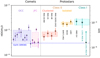 |
Fig. 3. Comparison of HDO/H2O ratios in comets and protostars. The values and references can be found in Table C.1. The equivalent D/H ratio is indicated on the right axis. For L1551 IRS5 N (vLSR ∼ 9 km s−1), the ratio is plotted for an excitation temperature of 300 K. |
Water observed in the warm inner regions of protostellar objects results from the thermal desorption of the icy grain mantles. Deuteration takes place early in the star formation process when the temperature is low and the density is relatively high. As a result, the gas phase HDO/H2O ratio observed in the warm regions of Class 0 objects should reflect those of the icy grain mantles. Consequently, the observed deuterium fractionation ratio at the Class I stage should either be similar to the Class 0 stage or decrease if water is partially reprocessed in the hot corino. In the latter case the deuteration process would not be efficient enough to increase or maintain the overall deuteration level. From the HDO/H2O ratio found in the high-velocity component of L1551 IRS5 we can conclude that the HDO/H2O ratio does not decrease and is still quite high, similarly to what is found for V883 Ori (Tobin et al. 2023) and SVS13-A (Codella et al. 2016).
A second conclusion is that the chemistry of L1551 IRS5 appears to be closer to isolated sources than to clustered sources. The similarity with isolated sources can be surprising at first sight, as L1551 IRS5 is part of the Taurus molecular cloud. However, it is located in the LDN 1551 group in the southern part of the cloud (e.g., Roccatagliata et al. 2020). This group shows a lower density of sources than other regions in Taurus (Gomez et al. 1993). The spatial density of sources in the Taurus molecular cloud is also much lower (only a few tens in ∼1 pc3, Gomez et al. 1993) than in Ophiuchus, which contains IRAS 16293−2422, and the NGC 1333 cloud in Perseus (a few 102–103, Bontemps et al. 2001; Jørgensen et al. 2006). As explained in Jensen et al. (2021), the higher water deuteration in isolated sources would be due to either a lower temperature or a longer prestellar phase compared to clustered sources. The environment around L1551 IRS5 could be colder than around IRAS 16293 and the NGC 1333 sources. The dense cores could also have more time to evolve before their collapse if L1551 IRS5 is on the edge of the cloud and if it is surrounded by fewer sources. As a consequence, the water deuteration in L1551 IRS5 would be closer to the Class 0 isolated sources. A similar explanation was proposed for the Class I protostar V883 Ori, which belongs to the Orion molecular cloud, but is in a relatively isolated area (Tobin et al. 2023). The lower values found in comets and in the protostars IRAS 16293−2422, NGC 1333 IRAS2A, IRAS4A, and IRAS4B suggest that our Solar System formed in a relatively dense clustered area. The similarity of the HDO/H2O ratio between the binary L1551 IRS5 and the singly Class I object V883 Ori also seems to indicate that the binarity does not influence the water deuteration.
In conclusion, this study highlights the importance of carrying out water deuteration measurements toward more sources, at different evolutionary stages, and in different environments in order to better understand the water formation and evolution during the formation process of solar-type stars. Investigations of the D2O/HDO ratio in Class I protostars would also be useful to check the similarity with Class 0 sources.
The D/H ratio of water is equal to 1/2 × HDO/H2O due to statistics.
CASSIS (http://cassis.irap.omp.eu/) has been developed by IRAP-UPS/CNRS.
Acknowledgments
The authors thank the IRAM staff, especially Jan Martin Winters and Jérémie Boissier for their help with the data reduction. This study is part of a project that has received funding from the European Research Council (ERC) under the European Union’s Horizon 2020 research and innovation programme under Grant agreement No. 949278 (Chemtrip) and Grant agreement No. 716155 (SACCRED). This work made use of Astropy: (http://www.astropy.org) a community-developed core Python package and an ecosystem of tools and resources for astronomy (Astropy Collaboration 2013, 2018, 2022).
References
- Altwegg, K., Balsiger, H., Bar-Nun, A., et al. 2015, Science, 347, 1261952P [NASA ADS] [CrossRef] [Google Scholar]
- Astropy Collaboration (Robitaille, T. P., et al.) 2013, A&A, 558, A33 [NASA ADS] [CrossRef] [EDP Sciences] [Google Scholar]
- Astropy Collaboration (Price-Whelan, A. M., et al.) 2018, AJ, 156, 123 [Google Scholar]
- Astropy Collaboration (Price-Whelan, A. M., et al.) 2022, ApJ, 935, 167 [NASA ADS] [CrossRef] [Google Scholar]
- Audard, M., Ábrahám, P., Dunham, M. M., et al. 2014, in Protostars and Planets VI, eds. H. Beuther, R. S. Klessen, C. P. Dullemond, & T. Henning, 387 [Google Scholar]
- Bianchi, E., Chandler, C. J., Ceccarelli, C., et al. 2020, MNRAS, 498, L87 [NASA ADS] [CrossRef] [Google Scholar]
- Biver, N., Bockelée-Morvan, D., Crovisier, J., et al. 2006, A&A, 449, 1255 [NASA ADS] [CrossRef] [EDP Sciences] [Google Scholar]
- Biver, N., Moreno, R., Bockelée-Morvan, D., et al. 2016, A&A, 589, A78 [NASA ADS] [CrossRef] [EDP Sciences] [Google Scholar]
- Bockelée-Morvan, D., Gautier, D., Lis, D. C., et al. 1998, Icarus, 133, 147 [CrossRef] [Google Scholar]
- Bockelée-Morvan, D., Biver, N., Swinyard, B., et al. 2012, A&A, 544, L15 [CrossRef] [EDP Sciences] [Google Scholar]
- Bonnarel, F., Fernique, P., Bienaymé, O., et al. 2000, A&AS, 143, 33 [NASA ADS] [CrossRef] [EDP Sciences] [Google Scholar]
- Bontemps, S., André, P., Kaas, A. A., et al. 2001, A&A, 372, 173 [NASA ADS] [CrossRef] [EDP Sciences] [Google Scholar]
- Brown, R. H., Lauretta, D. S., Schmidt, B., & Moores, J. 2012, Planet. Space Sci., 60, 166 [NASA ADS] [CrossRef] [Google Scholar]
- Carr, J. S., Harvey, P. M., & Lester, D. F. 1987, ApJ, 321, L71 [NASA ADS] [CrossRef] [Google Scholar]
- Ceccarelli, C., Caselli, P., Bockelée-Morvan, D., et al. 2014, in Protostars and Planets VI, eds. H. Beuther, R. S. Klessen, C. P. Dullemond, & T. Henning, 859 [Google Scholar]
- Chen, H., Myers, P. C., Ladd, E. F., & Wood, D. O. S. 1995, ApJ, 445, 377 [NASA ADS] [CrossRef] [Google Scholar]
- Cieza, L. A., Casassus, S., Tobin, J., et al. 2016, Nature, 535, 258 [Google Scholar]
- Cleeves, L. I., Bergin, E. A., Alexander, C. M. O. D., et al. 2014, Science, 345, 1590 [NASA ADS] [CrossRef] [Google Scholar]
- Codella, C., Ceccarelli, C., Bianchi, E., et al. 2016, MNRAS, 462, L75 [NASA ADS] [CrossRef] [Google Scholar]
- Connelley, M. S., & Reipurth, B. 2018, ApJ, 861, 145 [NASA ADS] [CrossRef] [Google Scholar]
- Coutens, A., Vastel, C., Caux, E., et al. 2012, A&A, 539, A132 [NASA ADS] [CrossRef] [EDP Sciences] [Google Scholar]
- Coutens, A., Jørgensen, J. K., Persson, M. V., et al. 2014, ApJ, 792, L5 [Google Scholar]
- Cruz-Sáenz de Miera, F., Kóspál, Á., Ábrahám, P., Liu, H. B., & Takami, M. 2019, ApJ, 882, L4 [CrossRef] [Google Scholar]
- Davies, J. K., Roush, T. L., Cruikshank, D. P., et al. 1997, Icarus, 127, 238 [NASA ADS] [CrossRef] [Google Scholar]
- de Laeter, J. R., Böhlke, J. K., Bièvre, P. D., et al. 2003, Pure Appl. Chem., 75, 683 [Google Scholar]
- Fischer, W. J., Hillenbrand, L. A., Herczeg, G. J., et al. 2022, arXiv e-prints [arXiv:2203.11257] [Google Scholar]
- Furuya, K., van Dishoeck, E. F., & Aikawa, Y. 2016, A&A, 586, A127 [NASA ADS] [CrossRef] [EDP Sciences] [Google Scholar]
- Gibb, E. L., Bonev, B. P., Villanueva, G., et al. 2012, ApJ, 750, 102 [NASA ADS] [CrossRef] [Google Scholar]
- Glorian, J.-M., Fernique, P., Allen, M., et al. 2021, in ADASS XXXI Conference Oct 2021 (Cape Town: ASP), ASP Conf. Ser. [Google Scholar]
- Goldsmith, P. F., Langer, W. D., & Velusamy, T. 1999, ApJ, 519, L173 [NASA ADS] [CrossRef] [Google Scholar]
- Gomez, M., Hartmann, L., Kenyon, S. J., & Hewett, R. 1993, AJ, 105, 1927 [NASA ADS] [CrossRef] [Google Scholar]
- Harsono, D., Persson, M. V., Ramos, A., et al. 2020, A&A, 636, A26 [NASA ADS] [CrossRef] [EDP Sciences] [Google Scholar]
- Hartogh, P., Lis, D. C., Bockelée-Morvan, D., et al. 2011, Nature, 478, 218 [Google Scholar]
- Hogerheijde, M. R., Bergin, E. A., Brinch, C., et al. 2011, Science, 334, 338 [Google Scholar]
- Hutsemékers, D., Manfroid, J., Jehin, E., Zucconi, J. M., & Arpigny, C. 2008, A&A, 490, L31 [NASA ADS] [CrossRef] [EDP Sciences] [Google Scholar]
- Jensen, S. S., Jørgensen, J. K., Kristensen, L. E., et al. 2019, A&A, 631, A25 [NASA ADS] [CrossRef] [EDP Sciences] [Google Scholar]
- Jensen, S. S., Jørgensen, J. K., Furuya, K., Haugbølle, T., & Aikawa, Y. 2021, A&A, 649, A66 [NASA ADS] [CrossRef] [EDP Sciences] [Google Scholar]
- Jørgensen, J. K., & van Dishoeck, E. F. 2010, ApJ, 725, L172 [Google Scholar]
- Jørgensen, J. K., Harvey, P. M., Evans, Neal J. I., et al. 2006, ApJ, 645, 1246 [CrossRef] [Google Scholar]
- Jørgensen, J. K., Müller, H. S. P., Calcutt, H., et al. 2018, A&A, 620, A170 [Google Scholar]
- Lis, D. C., Biver, N., Bockelée-Morvan, D., et al. 2013, ApJ, 774, L3 [NASA ADS] [CrossRef] [Google Scholar]
- Lis, D. C., Bockelée-Morvan, D., Güsten, R., et al. 2019, A&A, 625, L5 [NASA ADS] [CrossRef] [EDP Sciences] [Google Scholar]
- Mangum, J. G., & Shirley, Y. L. 2015, PASP, 127, 266 [Google Scholar]
- Meier, R., Owen, T. C., Matthews, H. E., et al. 1998, Science, 279, 842 [NASA ADS] [CrossRef] [Google Scholar]
- Mercimek, S., Codella, C., Podio, L., et al. 2022, A&A, 659, A67 [NASA ADS] [CrossRef] [EDP Sciences] [Google Scholar]
- Müller, H. S. P., Schlöder, F., Stutzki, J., & Winnewisser, G. 2005, J. Mol. Struc., 742, 215 [Google Scholar]
- Mumma, M. J., Weaver, H. A., Larson, H. P., Davis, D. S., & Williams, M. 1986, Science, 232, 1523 [CrossRef] [Google Scholar]
- Mundt, R., Stocke, J., Strom, S. E., Strom, K. M., & Anderson, E. R. 1985, ApJ, 297, L41 [NASA ADS] [CrossRef] [Google Scholar]
- Persson, M. V., Jørgensen, J. K., & van Dishoeck, E. F. 2013, A&A, 549, L3 [NASA ADS] [CrossRef] [EDP Sciences] [Google Scholar]
- Persson, M. V., Jørgensen, J. K., van Dishoeck, E. F., & Harsono, D. 2014, A&A, 563, A74 [NASA ADS] [CrossRef] [EDP Sciences] [Google Scholar]
- Pickett, H. M., Poynter, R. L., Cohen, E. A., et al. 1998, J. Quant. Spectr. Radiat. Transf., 60, 883 [NASA ADS] [CrossRef] [Google Scholar]
- Rivkin, A. S., & Emery, J. P. 2010, Nature, 464, 1322 [NASA ADS] [CrossRef] [Google Scholar]
- Roccatagliata, V., Franciosini, E., Sacco, G. G., Randich, S., & Sicilia-Aguilar, A. 2020, A&A, 638, A85 [NASA ADS] [CrossRef] [EDP Sciences] [Google Scholar]
- Takakuwa, S., Saigo, K., Matsumoto, T., et al. 2020, ApJ, 898, 10 [NASA ADS] [CrossRef] [Google Scholar]
- Taquet, V., López-Sepulcre, A., Ceccarelli, C., et al. 2013, ApJ, 768, L29 [NASA ADS] [CrossRef] [Google Scholar]
- Tobin, J. J., van’t Hoff, M. L. R., Leemker, M., et al. 2023, Nature, 615, 227 [NASA ADS] [CrossRef] [Google Scholar]
- Trigo-Rodríguez, J. M., Rimola, A., Tanbakouei, S., Soto, V. C., & Lee, M. 2019, Space Sci. Rev., 215, 18 [CrossRef] [Google Scholar]
- van der Tak, F. F. S., Black, J. H., Schöier, F. L., Jansen, D. J., & van Dishoeck, E. F. 2007, A&A, 468, 627 [NASA ADS] [CrossRef] [EDP Sciences] [Google Scholar]
- van Dishoeck, E. F., Kristensen, L. E., Mottram, J. C., et al. 2021, A&A, 648, A24 [NASA ADS] [CrossRef] [EDP Sciences] [Google Scholar]
- Villanueva, G. L., Mumma, M. J., Bonev, B. P., et al. 2009, ApJ, 690, L5 [NASA ADS] [CrossRef] [Google Scholar]
- Wilson, T. L., & Rood, R. 1994, ARA&A, 32, 191 [Google Scholar]
- Zucker, C., Speagle, J. S., Schlafly, E. F., et al. 2019, ApJ, 879, 125 [NASA ADS] [CrossRef] [Google Scholar]
Appendix A: Additional tables and figures on observations
Table A.1 lists the calibrators used for the different observations. Gaussian fitting was performed on the spectra to extract the fluxes of the HDO and  lines (see Figure A.1). A summary of the fit results is presented in Table A.2. We also performed circular Gaussian fitting of the emission lines in the (u,v)-plane to estimate the size of the sources. The results of the fits are summarized in Table A.3.
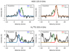 |
Fig. A.1. Gaussian line fits using the CASSIS software. The upper panel shows the spectra of the HDO transition at 225.9 GHz, while the lower panel is for the |

List of calibrators.
Gaussian fitting parameters and fluxes of the water isotopolog lines.
Results from the circular Gaussian fits performed in the (u,v)-plane.
Appendix B: Exploration of the physical parameters and the LTE assumption
B.1. Impact of source size and excitation temperature on HDO/H2O ratio
To investigate the impact of source size and excitation temperature on the HDO/H2O ratio derived for the component at 9 km s−1, we calculated the column densities needed to reproduce the fluxes of the HDO line at 225.9 GHz and the  line at 203.4 GHz for a wide range of excitation temperatures (100–300 K) and sizes (0.10–0.75″). The results of this method, which assumes LTE and optically thin lines, are presented in Figure B.1. The derived HDO/H2O ratio is not very sensitive to the excitation temperature and size as it ranges between 1.5 × 10⁻³ and 2.2 × 10⁻³. An analogous study done by Jørgensen & van Dishoeck (2010) led to similar conclusions.
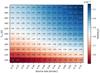 |
Fig. B.1. HDO/H2O ratios (× 10−3) obtained for the component at 9 km s−1 (N) of L1551 IRS5 as a function of different excitation temperatures and sizes assuming optically thin LTE emission. |
Figure B.2 shows how the HDO/H2O ratios of both components vary as a function of the excitation temperature when using the source sizes derived with circular Gaussian fitting of the lines in the (u,v)-plane.
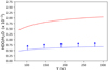 |
Fig. B.2. Evolution of HDO/H2O ratio as a function of excitation temperature assuming source sizes of 0.35″ and 0.45″ for the M and N positions, respectively. The solid red line represents the ratio found for N (component at 9 km s−1), while the blue dashed line is for M (6 km s−1). The arrows indicate lower limits. |
B.2. Non-LTE modeling
The LTE assumption has been tested and approved for the same transitions in other hot corinos (Persson et al. 2014; Coutens et al. 2014). We carried out a similar test for L1551 IRS5 using the non-LTE radiative transfer code RADEX (van der Tak et al. 2007) with the Large Velocity Gradient (LVG) expanding sphere method. We varied the temperature between 100 and 300 K, similarly to the LTE analysis. For the H2 density, we considered a range from 107 to 1011 cm−3. With a non-LTE analysis of three HDO lines, Coutens et al. (2014) derived a H2 density higher than 108 cm−3 in the warm inner regions of the low-mass protostar NGC1333 IRAS2A. The results are shown in Figure B.3. The HDO/H2O ratio derived with RADEX, (1.3 - 1.8) × 10−3 is in agreement with the LTE values within the uncertainties.
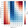 |
Fig. B.3. HDO/H2O ratio (× 10−3) obtained for the component at 9 km s−1 (N) of L1551 IRS5 with the non-LTE radiative transfer code RADEX as a function of the kinetic temperature and the H2 density. |
B.3. Modeling of the HDO line at 143.7 GHz and constraints on the excitation temperatures
The spectral resolution of the HDO transition at 143.7 GHz does not allow us to distinguish between the fluxes coming from the component at 6 km s−1 and the one at 9 km s−1. However, we can use the total flux to constrain the excitation temperatures for the two components. Assuming the source sizes obtained with the fits in the (u,v)-plane, we calculated the column densities of HDO needed to reproduce the two components at 225.9 GHz for various excitation temperatures. Then we predicted the expected flux at 143.7 GHz at 6 and 9 km s−1, and summed the two fluxes before comparing them to the observed flux (see Table A.2). Figure B.4 shows that a good agreement (< 20%) is only found if the excitation temperature for the component at 9 km s−1 is ≳ 240 K. The excitation temperature is not constrained for the component at 6 km s−1.
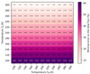 |
Fig. B.4. Percentage errors between the predicted and observed fluxes of the HDO line at 143.7 GHz as a function of excitation temperature for positions M and N. Source sizes of 0.35″ and 0.45″ are assumed for the M and N positions, respectively. |
Appendix C: Previous results on water deuteration
Table C.1 summarizes the HDO/H2O ratios determined in comets and protostars.
Water deuterium fractionation ratios determined in comets and protostars.
All Tables
Column densities and HDO/H2O ratio in L1551 IRS5 for different excitation temperatures.
All Figures
|
Fig. 1. Comparison of the spectra of the water isotopolog transitions. The green, blue, red, and orange solid lines represent the spectra extracted at the position S, M, N, and O, respectively. The dotted lines show velocities of 6.0 km s−1 (blue) and 9.5 km s−1 (red). Considering the synthetic beam sizes and the separation of the N and S components, the extracted spectra are not entirely independent from each other. For the HDO line at 143.7 GHz, the spatial resolution is too low to distinguish O from N and M from S. The x-axis scale is larger for this transition. |
| In the text | |
|
Fig. 2. Integrated emission maps of the HDO line at 225.9 GHz (top) and the |
| In the text | |
|
Fig. 3. Comparison of HDO/H2O ratios in comets and protostars. The values and references can be found in Table C.1. The equivalent D/H ratio is indicated on the right axis. For L1551 IRS5 N (vLSR ∼ 9 km s−1), the ratio is plotted for an excitation temperature of 300 K. |
| In the text | |
|
Fig. A.1. Gaussian line fits using the CASSIS software. The upper panel shows the spectra of the HDO transition at 225.9 GHz, while the lower panel is for the |
| In the text | |
|
Fig. B.1. HDO/H2O ratios (× 10−3) obtained for the component at 9 km s−1 (N) of L1551 IRS5 as a function of different excitation temperatures and sizes assuming optically thin LTE emission. |
| In the text | |
|
Fig. B.2. Evolution of HDO/H2O ratio as a function of excitation temperature assuming source sizes of 0.35″ and 0.45″ for the M and N positions, respectively. The solid red line represents the ratio found for N (component at 9 km s−1), while the blue dashed line is for M (6 km s−1). The arrows indicate lower limits. |
| In the text | |
|
Fig. B.3. HDO/H2O ratio (× 10−3) obtained for the component at 9 km s−1 (N) of L1551 IRS5 with the non-LTE radiative transfer code RADEX as a function of the kinetic temperature and the H2 density. |
| In the text | |
|
Fig. B.4. Percentage errors between the predicted and observed fluxes of the HDO line at 143.7 GHz as a function of excitation temperature for positions M and N. Source sizes of 0.35″ and 0.45″ are assumed for the M and N positions, respectively. |
| In the text | |
Current usage metrics show cumulative count of Article Views (full-text article views including HTML views, PDF and ePub downloads, according to the available data) and Abstracts Views on Vision4Press platform.
Data correspond to usage on the plateform after 2015. The current usage metrics is available 48-96 hours after online publication and is updated daily on week days.
Initial download of the metrics may take a while.