| Issue |
A&A
Volume 677, September 2023
|
|
|---|---|---|
| Article Number | A41 | |
| Number of page(s) | 13 | |
| Section | Atomic, molecular, and nuclear data | |
| DOI | https://doi.org/10.1051/0004-6361/202346967 | |
| Published online | 01 September 2023 | |
Gas phase Elemental abundances in Molecular cloudS (GEMS)
VIII. Unlocking the CS chemistry: The CH + S → CS + H and C2 + S → CS + C reactions
1
Laboratory for Astrophysics, Leiden Observatory, Leiden University,
PO Box 9513,
2300-RA,
Leiden, The Netherlands
2
Instituto de Física Fundamental (IFF-CSIC), C.S.I.C.,
Serrano 123,
28006
Madrid, Spain
e-mail: octavio.roncero@csic.es
3
University of Firat, Department of Physics,
23169
Elazig, Turkey
4
Institute of Physics, Faculty of Physics, Astronomy and Informatics, Nicolaus Copernicus University in Torun,
Grudziadzka 5,
87-100
Torun, Poland
5
Université Paris-Saclay, CEA, AIM, Département d’Astrophysique (DAp),
91191
Gif-sur-Yvette, France
6
Observatorio Astronómico Nacional (IGN),
c/ Alfonso XII 3,
28014
Madrid, Spain
7
Laboratoire d’astrophysique de Bordeaux, Univ. Bordeaux, CNRS,
B18N, allée Geoffroy Saint-Hilaire,
33615
Pessac, France
8
Institut des Sciences Moléculaires (ISM), CNRS, Univ. Bordeaux,
351 cours de la Libération,
33400
Talence, France
9
Sorbonne Université, Observatoire de Paris, Univerité PSL, CNRS, LERMA,
92190
Meudon, France
10
Centre for Astrochemical Studies, Max-Planck-Institute for Extraterrestrial Physics,
Giessenbachstrasse 1,
85748
Garching, Germany
11
Institut de Planétologie et d’Astrophysique de Grenoble (IPAG), Université Grenoble Alpes, CNRS,
38000
Grenoble, France
12
Institut de Radioastronomie Millimétrique (IRAM),
300 Rue de la Piscine,
38406
Saint-Martin-d’Hères, France
Received:
22
May
2023
Accepted:
29
June
2023
Context. Carbon monosulphide (CS) is among the few sulphur-bearing species that have been widely observed in all environments, including in the most extreme, such as diffuse clouds. Moreover, CS has been widely used as a tracer of the gas density in the interstellar medium in our Galaxy and external galaxies. Therefore, a complete understanding of its chemistry in all environments is of paramount importance for the study of interstellar matter.
Aims. Our group is revising the rates of the main formation and destruction mechanisms of CS. In particular, we focus on those involving open-shell species for which the classical capture model might not be sufficiently accurate. In this paper, we revise the rates of reactions CH + S → CS + H and C2 + S → CS + C. These reactions are important CS formation routes in some environments such as dark and diffuse warm gas.
Methods. We performed ab initio calculations to characterize the main features of all the electronic states correlating to the open shell reactants. For CH+S, we calculated the full potential energy surfaces (PESs) for the lowest doublet states and the reaction rate constant with a quasi-classical method. For C2+S, the reaction can only take place through the three lower triplet states, which all present deep insertion wells. A detailed study of the long-range interactions for these triplet states allowed us to apply a statistic adiabatic method to determine the rate constants.
Results. Our detailed theoretical study of the CH + S → CS + H reaction shows that its rate is nearly independent of the temperature in a range of 10–500 K, with an almost constant value of 5.5 × 10⁻¹¹ cm3 s−1 at temperatures above 100 K. This is a factor of about 2–3 lower than the value obtained with the capture model. The rate of the reaction C2 + S → CS + C does depend on the temperature, and takes values close to 2.0 × 10⁻¹⁰ cm3 s−1 at low temperatures, which increase to ~ 5.0 × 10⁻¹⁰ cm3 s−1 for temperatures higher than 200 K. In this case, our detailed modeling - taking into account the electronic and spin states – provides a rate that is higher than the one currently used by factor of approximately 2.
Conclusions. These reactions were selected based on their inclusion of open-shell species with many degenerate electronic states, and, unexpectedly, the results obtained in the present detailed calculations provide values that differ by a factor of about 2–3 from the simpler classical capture method. We updated the sulphur network with these new rates and compare our results in the prototypical case of TMC1 (CP). We find a reasonable agreement between model predictions and observations with a sulphur depletion factor of 20 relative to the sulphur cosmic abundance. However, it is not possible to fit the abundances of all sulphur-bearing molecules better than a factor of 10 at the same chemical time.
Key words: molecular processes / ISM: abundances / ISM: clouds / ISM: molecules
© The Authors 2023
 Open Access article, published by EDP Sciences, under the terms of the Creative Commons Attribution License (https://creativecommons.org/licenses/by/4.0), which permits unrestricted use, distribution, and reproduction in any medium, provided the original work is properly cited.
This article is published in open access under the Subscribe to Open model. Subscribe to A&A to support open access publication.
1 Introduction
Astrochemistry has become a necessary tool for understanding the interstellar medium (ISM) of our Galaxy and external galaxies. Nowadays, we are aware of the existence of nearly 300 molecules in the interstellar and circumstellar medium, as well as of around 70 molecules in external galaxies (for a complete list, see the Cologne Database for Molecular Spectroscopy1). Although the sulphur cosmic elemental abundance is only ten times lower than that of carbon (S/H ≈ 1.5 × 10⁻⁵), only 33 out of the currently detected interstellar molecules contain sulphur atoms. This apparent lack of chemical diversity in astrophysical sulphur-bearing molecules is the consequence of a greater problem in astrochemistry: there is an unexpected paucity of sulphur-bearing species in dense molecular clouds and star-forming regions. In such dense regions, the sum of the observed gas-phase abundances of sulphur-bearing species (the most abundant are SO, SO2, H2S, CS, HCS+, H2CS, C2S, C3S, and NS) constitutes only <1% of the expected amount (Agúndez & Wakelam 2013; Vastel et al. 2018; Rivière-Marichalar et al. 2019; Hily-Blant et al. 2022). One might postulate that most of the sulphur is locked on the icy grain mantles, but a similar trend is encountered within the solid phase, where s-OCS (the prefix “s-” indicates that the molecule is in the solid phase) and s-SO2 are the only sulphur-bearing species detected so far (Palumbo et al. 1995, 1997; Boogert et al. 1997; Ferrante et al. 2008), and only upper limits to the s-H2S abundance have been derived (Jiménez-Escobar & Muñoz Caro 2011). Recent observations with the James Webb Space Telescope (JWST) did not detect s-H2S either (McClure et al. 2023). According to these data, the abundances of the observed icy species account for <5% of the total expected sulphur abundance. This means that 94% of the sulphur is missing in our counting. It has been suggested that this missing sulphur may be locked in hitherto undetected reservoirs in gas and icy grain mantles, or as refractory material (Shingledecker et al. 2020). In particular, laboratory experiments and theoretical work shows that sulphur allotropes, such as S8, could be an important refractory reservoir (Jiménez-Escobar et al. 2014; Shingledecker et al. 2020; Cazaux et al. 2022).
Gas phase Elemental abundances in Molecular CloudS (GEMS) is an IRAM 30 m Large Program designed to estimate the S, C, N, and O depletions and the gas ionization fraction as a function of visual extinction in a selected set of prototypical star-forming filaments in low-mass (Taurus), intermediate-mass (Perseus), and high-mass (Orion) star forming regions (Fuente et al. 2019, 2023; Navarro-Almaida et al. 2020; Bulut et al. 2021; Rodríguez-Baras et al. 2021; Esplugues et al. 2022; Spezzano et al. 2022). Determining sulphur depletion is probably the most challenging goal of this project. The direct observation of the potential main sulphur reservoirs (s-H2S, s-OCS, gas-phase atomic S) remains difficult even in the JWST era. Therefore, the sulphur elemental abundance needs to be estimated by comparing the observed abundances of rarer species, such as CS, SO, HCS+, H2S, SO2, and H2CS, with the predictions of complex gas-grain chemical models. In summary, the above factors mean that the sulphur chemistry in cold dark clouds remains a puzzling problem. The development of accurate and complete sulphur chemical networks is therefore required in order to disentangle the sulphur elemental abundance. Within the context of the GEMS project, we carried out a large theoretical effort to improve the accuracy of key reaction rates of the sulphur chemical network, paying special attention to those associated with the formation and destruction paths of SO and CS, which are the gas-phase sulphur-bearing species observed in more different environments. We estimated the rates of the reactions S + O2 → SO + O (Fuente et al. 2016) and SO + OH → SO2 + H (Fuente et al. 2019) at the low temperatures prevailing in dark clouds. These reactions drive the SO chemistry in these cold environments. Bulut et al. (2021) estimated the rate constant of the CS + O → SO + O reaction, which has been proposed as an efficient CS destruction mechanism in molecular clouds. In the present work, we study two formation reactions of CS, which are thought to be important in regions with a low ionization fraction: CH(2Π) + S(3P) and  . In both cases, the two reactants are radicals presenting several degenerate or quasi-degenerate electronic states: for CH + S, there are 36 degenerate states and for C2 + S, the first excited C2(3Πu) states are only 0.089 eV above the
  ground state. This makes the experimental determination of their rates difficult, because of the low densities in which two radical species are obtained, and because of the possibility of self-reactions. Therefore, the most accurate theoretical determination of the reaction rate constants is desirable in order to place satisfactory constraints on the abundance of CS in chemical models.
The reactions rates currently available for these two reactions were obtained with a classical capture method (Vidal et al. 2017). Dealing with open-shell systems, there are several degenerate electronic states for the reactants, not all of them leading to the desired product, and the crossing among them leads to barriers. All these effects are ignored in the classical capture method. Precise calculations like the ones in this article are needed to improve the accuracy of our chemical networks and to estimate the uncertainties associated with the less demanding classical capture methods.
2 CH+S reaction

presents several rearrangement channels (CS and SH products) with several electronic states in each case. There are 36 degenerate states (neglecting spin-orbit couplings) in the CH(2Π) + S(3P) entrance channel. There are the same number of degenerate states in the SH(X2Π) + C(3P) rearrangement channel, which is only ≈0.08 eV below CH(2Π) + S(3P). The reaction  has already been studied theoretically for the ground 2A′ state (Stoecklin et al. 1988, 1990a,b; Voronin 2004; Song et al. 2016) and for the excited 2A″ state (Zhang et al. 2018).
The 36 degenerate electronic states (neglecting spin-orbit couplings) involved in Eq. (1a) consist of 6 spin states times 6 orbital states. The spin states are quartet and doublets, while the orbital states are split into A′ and A″ states, that is, symmetric or antisymmetric with respect to the inversion through the plane of the molecule. Of all these 36 states, only one doublet (i.e. 2 states) correlates to the CS(X1Σ+) states, which correspond to the ground adiabatic 2A′ states. Reaction (1a) toward the X1Σ+ is exothermic by ≈3.5 eV. However, the excited CS(a3Π) is about 3.42 eV above CS(X1Σ+), and the reaction is nearly thermoneutral.
2.1 Ab initio calculations
Here, to describe the electronic correlation along the reaction, we use the internally contracted multi-reference configuration interaction (ic-MRCI) method (Werner & Knowles l988a,b), including the Davidson correction (hereafter referred to as MRCI+Q; Davidson 1975) and the calculations are performed with the MOLPRO suite of programs (Werner et al. 2012). Three electronic states are calculated for each symmetry, 3 2A′ and 3 2A″, and the same is true for the quartet states.
In these calculations, the molecular orbitals are optimized using a state-averaged complete active space self-consistent field (SA-CASSCF) method, with an active space of ten orbitals (seven a′ symmetry and three a″ symmetry). Five 2,4A′ and four 2,4A″ electronic states are calculated and simultaneously optimized at CASSCF level using a dynamical weighting factor of 10. In all these calculations, the aug-cc-pVTZ (aVTZ) basis set is used (Dunning 1989). For the ic-MRCI calculations, six orbitals are kept doubly occupied, giving rise to ~5 × 10⁶ (382 × 106) contracted (uncontracted) configurations. Checks made with the aug-cc-pVQZ basis gave nearly parallel results along some of the minimum energy paths (MEPs) shown below. For this reason, we kept the aVTZ basis set to build the PES. Nevertheless, to better describe the long-range part, we use a AV5Z basis, as discussed below.
Figure 1 shows the first five A′ and four A″ states for doublet (bottom) and quartet (top) multiplicities calculated at CASSCF level. With no spin-orbit couplings, the six electronic states for each multiplicity are degenerate for long distances of between S(3P) and CH(X2Π), and this asymptote is taken as the origin of energy. When they approach one another, they cross with the excited states correlating to S(3P) + CH(a4Σ−). After the crossing, there are three (two) curves for the doublet (quartet) states that become negative. For the doublets, one of these states correlates to CS(X1Σ+) and two correlate to CS(a3Πr) states.
This degeneracy is recovered in the MRCI+Q calculations shown in Fig. 2. The two degenerate states, 12A′ and 12A″ (and 14A′ and 14A″ for quartets), correspond to the HCS(2Π) radical (and the excited HCS(4Π)) state, which experience Renner-Teller effects, as studied by Senekowitsch et al. (1990). In the case of doublets, the X2A′ state (of 2Π character at collinear geometry) crosses with 22A′ (of 2Σ character at collinear geometry), which correlate with the CS(X1Σ+) state of the products.
The crossing at collinear geometry is a conical intersection between Σ and Π states. As long as the system bends, there are couplings and the crossing is avoided. As a consequence, the ground X2A′ state correlates to the CS(X1Σ+) products, that is, only these two doublets among the 36 states correlating to the CH(2Π)+S(3P) reactants. Therefore, only the ground electronic state is needed to describe the reaction (1). The energy difference between the CH(2Π)+S(3P) and CS(X1Σ+) + H at their corresponding equilibrium geometries is De = 3.52 eV, and D0 = 3.62 eV when including zero-point energy (using the fit described below). As there have been no direct measurements for this reaction, the experimental exothermicity is estimated from the dissociation energies  , using the values reported by Huber & Herzberg (1979), and this D0 is about 10% higher than the present results.
2.2 Long-range interaction
MRCI calculations are not size consistent and the Davidson correction (+Q) is not adequate to describe closely lying electronic states. Therefore, the MRCI+Q method introduces inaccuracies in the long-range region, which need to be described accurately in order to obtain good rate constants at low temperatures. Coupled cluster methods are size consistent and are typically considered to be the best way to describe long-range interactions; however, in the presence of two open shell reactants, even these methods are not expected to yield good accuracy.
Here, as an alternative, we use the CASSCF method with a larger aV5Z basis set (Dunning 1989). Several points have been calculated in Jacobi coordinates, for CH(rCH) = 1.1199 Å and R = 10–50 Å, where R is the distance between the CH center of mass and the S atom as a function of the angle θ, with cos 9 = R · rCH/RrCH. At long distances, the system behaves as a dipole-quadrupole interaction, with the dipole of CH interacting with the quadrupole of a P sulphur atom whose analytical form is (Zeimen et al. 2003)
 (2)
(2)
with MQD(θ) and MQQ(θ) being 3×3 matrices, depending on Legendre polynomials (Zeimen et al. 2003). The eigenvalues of this matrix properly describe the angular dependence of the adiabatic states. Therefore, only two effective parameters are needed to fit the ab initio points, QAdB = 0.293 hartreeÅ−4 and QAQB = 0.092 hartree Å−5. Two families of three states are considered separately, namely 12A″, 12A′, 22A″ and 22A′, 32A′, 32A″, corresponding to the two Π states of CH interacting with the three P states of sulphur. The excellent agreement between calculated and fitted analytical expressions, as shown in Fig. 3, demonstrates the adequacy of the analytical fit in the asymptotic region.
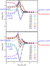 |
Fig. 1 CASSCF energies along the reaction coordinate defined as the RCS-RCH distance difference. The energies shown here are obtained for an angle γSCH = 179.9° for the doublet (bottom panel) and quartet (top panel) states for the CH + S → CS + H reaction. Here, we consider five A′ and four A″ electronic states. |
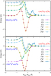 |
Fig. 2 MRCI+Q energies along the reaction coordinate defined as the RCS-RCH distance difference. The energies shown here are obtained for an angle γSCH = 179.9° for the doublet (bottom panel) and quartet (top panel) states, for the CH + S → CS + H reaction. Three A′ and three A″ electronic states are considered in each case. |
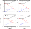 |
Fig. 3 Angular dependence of the long-range interaction between CH and S in the three lower electronic states. Points are the CASSCF(aV5Z) energies (in cm−1) as a function of the Jacobi angle 9 (defined in the text) for rCH = 1.1199 Å and R = 10, 15, 20 and 30 Å, as indicated in each panel, for the 12A″, 12A′, and 22A″ states. Lines correspond to the long-range analytical fit of Eq. (2) taken from Zeimen et al. (2003). |
2.3 Analytical fit of the ground state
The analytical representation of the potential energy surface of the ground 1 2A′ electronic state is described by two terms
 (3)
(3)
where V3B is the three-body term added to the zero-order description provided by the lowest root,  , of the 3×3 reactive force-field matrix defined as (Zanchet et al. 2018; Roncero et al. 2018; Goicoechea et al. 2021)
 (4)
(4)
The diagonal terms describe each of the rearrangement channels, in which VCH(rCH), VCS(rCS), and VSH(rSH) are fitted using the diatomic terms of Aguado & Paniagua (1992). In the reactant channel 1, the long-range term given by Eq. (2) is included. WAB are Morse potentials whose parameters are determined to describe each channel independently. Finally, the nondiagonal terms Vij are built as Gaussian functions  depending on the energy difference between the diagonal terms of the corresponding force-field matrix. The parameter α is determined to fit the transition between rearrangements.
The three-body term V3B in Eq. (3) is described with the method of Aguado & Paniagua (1992) using a modification of the program GFIT3C (Aguado et al. 1998). We included about 7500 ab initio points calculated at MRCI+Q level in the fit. These points are mainly composed of a grid of 22 points for 0.6 ≤ rCH ≤ 8 Å, 27 points for 1 ≤ rCS ≤ 8 Å, and 19 points in the θHCS angle, in intervals of 10°. The points are weighted with a weight of 1 for those with energy up to 1 eV from the entrance CH+S channel at 50 Å, and with a Gaussian function for higher energies, considering a minimum weight of 10−4. The final fit uses polynomials up to order 10, with an overall root-mean-square error of 0.07 eV.
The main features of the potential fit are shown in Fig. 4, where the contour plots for the reactants (bottom panel, for RCH = 1.1199 Å) and products (top panel, for RCS = 1.568 Å, and shifted by 3.526 eV, which is the exoergicity of the reaction) are shown. The CH+S reactant channel (bottom panel) is attractive for RCS < 7 Å, leading to the products channel at RCS ≈ 1.5 Å, with an energy of −5.5 eV. These energies correspond to the CS-H well in the products channel, which is about 2 eV below the CS + H products shown in the top panel of Fig. 4, which have been shifted by 3.526 eV to show the details. At RCH ≈ 2 Å, there is a barrier that arises from the curve crossing discussed above.
2.4 Quasi-classical versus quantum wave packet dynamics in the 12A′ state
To check the validity of the quasi-classical method, we first compare quantum and quasi-classical trajectory (QCT) calculations for total angular momentum J = 0. The quantum wave packet (WP) calculations are performed with the MADWAVE3 code (Zanchet et al. 2009) and the parameters used are listed in Table 1. The WP method is considered numerically exact but is very computationally demanding. The QCT calculations are performed with the MDwQT code (Sanz-Sanz et al. 2015; Zanchet et al. 2016; Ocaña et al. 2017). Initial conditions are sampled with the usual Monte Carlo method (Karplus et al. 1965). In this first set of calculations, CH is in its ground vibrational (v) and rotational state, (υ, j) = (0, 0), and the initial internuclear distance and velocity distributions are obtained with the adiabatic switching method (Grozdanov & Solov’ev 1982; Qu & Bowman 2016; Nagy & Lendvay 2017). We consider an impact parameter b = 0, which corresponds to J = 0. The initial distance between sulfur and the CH center of mass is set to 50 Bohr, and the trajectories are stopped when any internuclear distance is greater than 60 Bohr. For each energy, Ntot = 104 trajectories are run to calculate the reaction probability as PR(E) = Nr/Ntot, where Nr is the number of reactive trajectories.
The WP and QCT reaction probabilities are compared in Fig. 5, and the results from the two methods show very similar behavior: a reaction probability slightly higher than 0.9 at energies below 0.01 eV, decreasing as a function of collision energy down to a probability of lower than 0.2 at 1 eV. In the two cases, there are oscillations, which do not match perfectly but show similar envelopes. As these oscillations are expected to wash out when considering the partial wave summation over total angular momentum, J, we consider this agreement to be satisfactory. This leads us to conclude that the QCT method is sufficiently accurate to determine the reaction rate constant, as described below.
The reaction rate constant for CH(υ = 0 and 1) in the 12A′ electronic state is evaluated according to
 (5)
(5)
where bmax(T) and Pr(T) are the maximum impact parameter and reaction probability at constant temperature, respectively. In this case, about 105 trajectories are run for each temperature, which is also true for translation and rotation degrees of freedom, fixing the vibrational state of CH to υ = 0 or 1.
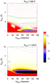 |
Fig. 4 Contour plots of the analytical potential energy surfaces fitted to ab initio points, corresponding to the reactant channel for RCH = 1.1199 Å (bottom panel) and to the products channel for RCS = 1.568 Å (top panel). Energies are in eV. For the products, the energies are shifted by 3.526 eV, so that their point of zero energy corresponds to the CS(req) at an infinite distance from H. The contours correspond to 0 and ± 1 meV in order to show the dependence of the potential at long distances. The units of the color box are eV. |
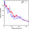 |
Fig. 5 CH+S → CS + H reaction probabilities versus collision energy for J = 0 in the 1 2A′ electronic state using quantum wave packet and quasi-classical trajectory methods. |
Parameters used in the wave packet calculations in reactant Jacobi coordinates.
2.5 Thermal rate
Considering that only the double degenerate 12A′ electronic state reacts to form CS(X1Σ+), the electronic partition function has to be considered. Neglecting the spin-orbit splitting, the electronic partition function would be 2/36, that is, the thermal rate constant is about 1/18 of the reaction rate,  , associated to the 1 2A′ state. Including the spin-orbit splitting of the
  sulphur atom, and assuming that only the lowest two spin-orbit states react (having an individual rate constant equal to
  ), the vibrational selected thermal rate constant is given by
![${K_\upsilon }\left( T \right) = {{2K_\upsilon ^{{1^2}A'}\left( T \right)} \over {4\left[ {5 + 3{\rm{exp}}\left( {{{ - 539.83} \mathord{\left/ {\vphantom {{ - 539.83} T}} \right. \kern-\nulldelimiterspace} T}} \right) + \exp \left( {{{ - 825.34} \mathord{\left/ {\vphantom {{ - 825.34} T}} \right. \kern-\nulldelimiterspace} T}} \right)} \right]}},$](/articles/aa/full_html/2023/09/aa46967-23/aa46967-23-eq15.png) (6)
(6)
and is shown in Fig. 6. In this figure, the red line corresponds to the rate constant (1.4 × 10⁻¹⁰ cm3 s−1) obtained from the KIDA data base, as obtained with a classical capture model (Vidal et al. 2017), using analytical formulas (Georgievskii & Klippenstein 2005; Woon & Herbst 2009) with dipole moments and polarizabilities taken from the literature or calculated using density functional theory.
The  rate constant at 10 K is about 4× 10⁻¹¹ cm3 s−1, increasing to a nearly constant value of ≈5.5× 10⁻¹¹ cm3 s−1 at temperatures above 100 K. This is a factor of between 2 and 3 lower than the value obtained with the capture model (Vidal et al. 2017).
When including the spin-orbit splitting, the rate Kυ=0(T) is larger at 10 K, simply because the populations of the excited sulphur spin-orbit states, JS = 1 and 0, are negligible. As temperature increases, their populations increase, leading to a reduction of the rate constant Kυ=0(T), which decreases tending to  at high temperature. The rate with spin-orbit splittings, Kυ=0(T), is only a factor ≈l/2 smaller than that of KIDA at 10 K, and is considered the most accurate obtained here. The Kυ=0(T) rate constant has been fitted and the parameters are listed in Table 2.
We also show  in Fig. 6. Its contribution at low temperatures is small, because the vibration energy of CH(v = 1) is about 0.337 eV higher than υ = 0, that is, 3916 K. Therefore, Kυ=0(T) is a good approximation of the thermal rate constant, which includes the spin-orbit splitting.
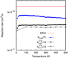 |
Fig. 6 Vibrational-selected rate constant for the CH(X2Π,v = 0) + S(3P) → CS(X1Σ) + H reaction, obtained here according to Eq. (6). |
Parameters used to fit the total reaction rates calculated for CH+S and C2 + S, according to the expression K(T) = A(T/300)Be−C/T
 |
Fig. 7 CASSCF/aVTZ optimized reaction paths for the conversion between C2+S and CS+C, which occurs on several potential energy surfaces of CCS. The reaction coordinate is defined as RCS−RCC, while the valence angle, γCCS, was held fixed at 179.9° in the geometry optimizations. Five A″ and four A′ electronic states of CCS were considered for each multiplicity: triplet (bottom panel), singlet (middle panel), and quintet (top panel). |
3 C2+S reaction

is exothermic by ~ 1 eV (Visser et al. 2019; Reddy et al. 2003). Due to the open-shell nature of the involved atoms [S(3P) and C(3P)], reactant collision and product formation can take place adiabatically on three triplet CCS potential energy surfaces (23A″+13A′); see, for example, Figs. 7 and 8. To the best of our knowledge, there have been no theoretical studies dedicated to this reaction. Vidal et al. (2017) reported a theoretical upper limit for its rate coefficient (k ~ 2 × 10⁻¹⁰ cm3 molecule−1 s−1 at 10 K) using classical capture rate theory. From an experimental viewpoint, presently available techniques for the production of reactant dicarbon often generate a mixture of both  and C2(a3Πu) (Gu et al. 2006; Páramo et al. 2008). It is important to note that this electronically excited state lies only ~ 716 cm−1 above the ground X form, which – together with the expected high reactivity of C and S atoms – make the laboratory characterization of this specific reaction (7) extremely cumbersome.
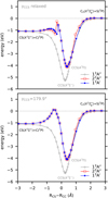 |
Fig. 8 Optimized reaction paths for |

3.1 Ab initio calculations
The methodology we employed to obtain optimized energy paths for the C2 + S → CS + C reaction closely resembles that used for the CH + S system. Our preliminary PES explorations and geometry optimizations were all performed at the SA-CASSCF level of theory, followed by single-point MRCI+Q calculations. The CASSCF active space involves a total of 14 correlated electrons in 12 active orbitals (9a′ + 3a″). For each multiplicity considered (triplet, singlet and quintet), we treated five A″ and four A′ electronic states simultaneously in the SA-CASSCF wave functions. The aVXZ (X = T, Q) basis sets of Dunning and co-workers (Dubernet & Hutson 1994; Kendall et al. 1992) were employed throughout, with the calculations done with MOLPRO.
Our calculated CASSCF/aVTZ optimized path for reaction (7) is shown in the bottom panel of Fig. 7. As seen, the  reactant collision involves only triplet CCS PESs and can happen on two 3A″ and one 3A′ electronic states. Proceeding through the ground-state PES of CCS(13A″), reaction (7) does not encounter any activation barriers for collinear atom-diatom approaches, being exothermic by ~ 0.6 eV at CASSCF/aVTZ level. We note that this process occurs via the formation of a strongly bound intermediate complex corresponding to the linear global minimum of CCS, ℓ-CCS(X3Σ−) (Saito et al. 1987); from this structure, the ground-state CS(X1Σ+) + C(3P) products can be directly accessed, without an exit barrier.
A close look at Fig. 7 (bottom panel) also reveals that the excited 23A″ and 13A′ electronic states are degenerate along C∞υ atom-diatom collisions. These PESs form the Renner-Teller components of the strongly bound ℓ-CCS(A3Π) complex, showing a conical intersection with ℓ-CCS(X3Σ−) at RCS −RCC ≈ +0.5 Å (Riaplov et al. 2003; Tarroni et al. 2007). As opposed to the ground 13A″ state, the conversion from reactants to products as proceeding adiabatically through the 23A and 13A′ PESs entails a large activation barrier (≈ 1 eV at CASSCF/aVTZ level), which is located at RCS − RCC ≈ −0.5 Å; see Fig. 7. As shown, this region of the nuclear configuration space is extremely congested by the existence of several low-lying excited triplet states correlating with C2(a3Πu) + S(3P). We note that the C2(a3Πu) + S(3P) reactants can approach each other in six triplet (33A″ + 33A′), six singlet (31 A″ + 31 A′), and six quintet (35A″ + 35A′) electronic states. For completeness, their corresponding optimized reaction paths toward CS+C formation are also plotted in Fig. 7; see bottom, middle, and top panels therein. Accordingly, when proceeding adiabatically, the reactions involving C2(a3Πu) + S(3P) are all endothermic, ultimately leading to excited-state CS+C products. These are therefore are expected to be highly inefficient at the low temperature regimes envisaged here (unless nonadiabatic transitions play a role) and are not considered further in this work for this reason.
Maintaining our focus on the target  process (reaction (7)) and to better estimate its overall attributes, we performed MRCI+Q/aVQZ//CASSCF/aVQZ calculations along the underlying reaction paths on 13A″, 23A″, and 13A′ electronic states. The results are plotted in Fig. 8. Accordingly, at this level of theory, our best estimate for the exothermicity of reaction (7) is 1.05 eV (without zero-point energy), a value that almost perfectly matches the corresponding experimental estimate of 1.04 eV (Visser et al. 2019; Reddy et al. 2003). The stabilization energies of the ℓ-CCS(X3Σ−) and ℓ-CCS(A3Π) complexes are herein predicted to be −5.3 and −4.2 eV, respectively, relative to the
  reactant channel. Most notably, Fig. 8 (bottom panel) shows that, at MRCI+Q/aVQZ//CASSCF/aVQZ level, the predicted activation barriers along linear C∞υ paths for the 23A″ and 13A′ states are largely reduced with respect to CASSCF/aVTZ values (Fig. 7; bottom panel), going from ≈ 1 to less than 0.1 eV. Indeed, by allowing the valence C−C−S angle (γCCS) to also be freely optimized in the MRCI+Q/aVQZ//CASSCF/aVQZ calculations, Fig. 8 (top panel) unequivocally shows that such barriers actually become submerged, lying below the corresponding
  reactant channel; we note the existence of small discontinuities on the ab initio curves that are associated with abrupt changes in γCCS near the top of these barriers. This clearly indicates that all such PESs (13A″, 23A″, and 13A′) contribute to the overall dynamics and kinetics of reaction (7), even at low temperatures. In the following, we describe the methodology employed to obtain rate coefficients for this target reaction.
3.2 Long-range interactions
Restricting the calculations to the equilibrium distance of  allows us to consider
  and C2(3Π) separately. Under this approximation, the situation simplifies to a closed shell diatom plus an open shell atom for the two asymptotes C2 + S and CS + C. For both cases, let us adopt the Jacobi coordinate system and expansion in terms of orthogonal functions as defined, for example, in Flower & Launay (1977); Dubernet & Hutson (1994):
 (8)
(8)
where  are spherical harmonics in Racah normalization. The θ, ϕ angles correspond to the orientation of diatomic molecules with respect to the vector connecting the center of mass of the diatomic molecule with the atom in a Jacobi frame, while θa, ϕa angles correspond to the orientation of the doubly occupied p orbital of the S and C atom, respectively. The R is the distance between the center of mass of the diatom and the atom. For both systems in Cs symmetry, the solution of the electronic Schrödinger equation is hard, because single-reference methods cannot be used due to the fact that two solutions will always belong to the same irreducible representation, and are nearly degenerate. The situation is simpler in the case of symmetric configurations: C∞υ (linear) for both systems, and C2υ (T-shaped) for C2 + S. For these cases, atom+diatom states belong to distinct irreducible representations: for linear geometry Π and Σ− states, while for C2υ these symmetries are B1, B2, and A2. For these particular configurations of the CCS system, the single-reference gold-standard CCSD(T) method can be used for calculations of interaction energy in each symmetry (Alexander 1998; Klos et al. 2004; Atahan et al. 2006).
Using linear and T-shape geometries, we calculated UCCSD(T) interaction energies in the range of 6–30 Å and converted them to  potentials using the following formula for C2+S,
 (9)
(9)
 (10)
(10)
 (11)
(11)
 (12)
(12)
and the following formula for CS+C,
 (13)
(13)
 (14)
(14)
 (15)
(15)
 (16)
(16)
where, in the latter equation, VΠ,0/VΣ,0 and VΠ,180/VΣ,180 denote the potential for appropriate symmetry in the C−S−C and C− C−S configurations, respectively. The above equations can be obtained by calculating Eq. (8) for θ, ϕ, θa, ϕa, which correspond to symmetric configurations (Flower & Launay 1977).
The  potentials were then carefully fitted to an analytical form in order to obtain the inverse power expansion form. It is important to take into account that collision-induced rotations of CS molecules are driven directly by V100 and V120 terms, while for C2 molecules colliding with atoms, the driving terms are V200 and V220. When the atoms are assumed to be spherically symmetric, the terms V120 and V220 can be ignored. Therefore, hereafter we skip the dependence on θa, ϕa in Eq. (8). Thus, our model of the potential used for the statistical method includes only the isotropic term V000 and the leading anisotropies V100 and V200, which were fitted to analytical forms of van der Waals expansion:
  for V000 and V200, and
  for V100. These potentials can be viewed as averaged over all orientations of P-state atoms. Moreover, for the leading coefficients, we also performed similar calculations using open-shell symmetry adapted perturbation theory (Hapka et al. 2012) and confirm the values for the leading coefficients C6 and C7 of the reactants and products (these agree to within 10%).
The final analytical form of the potential used for C2 + S reads (in atomic units of distance and energy)
 (17)
(17)
with A = −125.8, B = −9.444 × 10³, C = 1.743 × 10⁵, D = −13.66, E = −2.848 × 10³, and F = −1.929 × 10⁵, while for CS+C,
 (18)
(18)
with A = −147.5, B = −207.3, C = −3.834 × 10⁶, D = −2.805 × 10⁸, E = −487.3, F = −4.309 × 10³, G = −2.394 × 10⁷, and H = −1.997 × 10⁹.
3.3 Rate constant calculations
Due to the deep well appearing for the three lowest adiabatic states of the C2 + S reaction, and the large masses of the three atoms involved, this system has a high density of resonances near the thresholds. Therefore, this reaction is expected to be governed by a statistical mechanism. In this work, we use the adiabatic statistical (AS) method (Quack & Troe 1974), using the recently implemented (Gómez-Carrasco et al. 2022) AZTICC code. Here, we use the rigid rotor approach, which is similar to the method used to treat several reactions and inelastic processes (Konings et al. 2021). We consider the experimental exoergic values of  (Huber & Herzberg 1979), which already includes the vibrational zero-point energy (ZPE) of reactants and products. This exothermicity is very close to that shown in the ab initio calculations in Fig. 8, namely of ≈1 eV, which does not include ZPE.
In the rigid rotor approach, the diatomic distances for the diatomic molecules are frozen to their equilibrium values, namely re = 1.2425 and 1.568 Å for C2 and CS, respectively. As C2 is homonuclear, the even and odd rotational channels are not coupled, and are treated independently. The large exothermicity requires the inclusion of vibrational levels for the CS products of up to υ = 15 in order to adequately describe the density of states of the products. To this end, the adiabatic potentials are generated for each final υ independently using the rigid rotor approximation at req with the same long-range potential but shifting the energy using the anharmonic vibration constants, ωe = 0.15933 eV ωeχe = 0.801 meV from Herzberg (1950).
All product ro-vibrational levels are then considered to obtain the square of the S-matrix at each total angular momentum J (see Gómez-Carrasco et al. 2022 for more details). The calculations are done using a body-fixed frame, in which the z-axis is parallel to the Jacobi vector R, joining the diatomic center of mass to the atom, and the three atoms are considered in the body-fixed xz-plane. In the present calculations, a maximum rotational quantum numbers of jmax = 200 and 250 are considered for C2 and CS, respectively, together with a maximum helicity quantum number of Ωmax = 15. The individual state-to-state reactive cross sections are obtained by performing the summation over all J in the partial wave expression up to Jmax = 200.
Finally, integrating over the translational energy according to a Boltzmann energy distribution, and summing over all accessible states, the thermal rate constants, Kα(T), are obtained, with α = 13A″, 13A′, and 13A′. The 23A″ and 13A′ states present a submerged barrier, which could reduce the reactivity; however, here we consider that the three α electronic states have the same reactive rate constant. For this reason, when the spin-orbit splitting of S(3PJ) is included, the final thermal rate constant averaging over the spin-orbit states, KAS(T), is equal to Kα(T), as shown in Fig. 9; the rate constants have been fit to a modified Arrhenius expression and the parameters obtained are listed in Table 2.
The C2 + S → CS + S available in the KIDA data base2 is that of Vidal et al. (2017), and corresponds to a value of KC(T) = 2 10−10 cm3 s−1, which is independent of temperature, and was calculated using a capture method, that is, assuming that the reaction is exothermic, but without considering the deep well described in this work. Such an approach neglects the possibility that the C2S complex formed under the statistical assumption can exit back to C2 + S products. This probability is small because it is proportional to the density of states in each channel, and this density is much lower in the C2 + S due to the exothermicity, the homonuclear symmetry, and the larger rotational constant.
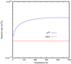 |
Fig. 9 Reactive rate constant for the C2 + S → CS + S collisions obtained with the present AS method and compared to that available in the KIDA database from Vidal et al. (2017). |
4 Discussion
In this section, we evaluate the impact of the new reaction rates on our understanding of interstellar chemistry. This is not straightforward, because the formation and destruction routes of the different species depend on local physical and chemical conditions, as well as the chemical time. We therefore need to consider different environments in order to obtain a comprehensive view of the impact of the new reactions rates on astrochemical calculations, and in particular on our ability to reproduce the abundance of CS.
We performed chemical calculations using Nautilus 1.1 (Ruaud et al. 2016), a three-phase model in which gas, grain surface, and grain mantle phases, and their interactions, are considered. We used the code upgraded as described by Wakelam et al. (2021), with the chemical network of KIDA2, which has been modified to account for the reaction rates estimated by Fuente et al. (2016, 2019), and this paper (reaction rates in Table 2). In Nautilus, desorption into the gas phase is only allowed for the surface species, considering both thermal and nonthermal mechanisms. In the regions where the temperature of grain particles is below the sublimation temperature, nonthermal desorption processes become important when calculating the number of molecules in gas phase. The latter includes desorption induced by cosmic rays (Hasegawa & Herbst 1993), direct (UV field), and indirect (secondary UV field induced by the cosmic-ray flux) photo-desorption, and reactive chemical desorption (Garrod et al. 2007; Minissale et al. 2016). In the following calculations, we use the prescription proposed by Minissale et al. (2016) for ice-coated grains to calculate the reactive chemical desorption. The physical and chemical conditions associated with these three simulations are detailed below:
TMC 1: This case represents the physical and chemical conditions prevailing in molecular cloud complexes where low-mass stars are formed. The physical properties of these regions are typically described with moderate number densities of atomic hydrogen nuclei nH = 3 × 104 cm−3, cold gas and dust temperatures T = 10 K, a moderate visual extinction AV = 20 mag, a cosmic-ray H2 ionization rate of ζH2 = 10−16 s−1 (Fuente et al. 2019, 2023), and an intensity of the far-ultraviolet (FUV) field equal to χ = 5 in Draine units. We assume that sulphur is depleted by a factor of 20 relative to the cosmic abundance as derived by Fuente et al. (2019, 2023) in Taurus and Perseus.
Hot core: This case represents the physical and chemical conditions in the warm interior of young protostars where the gas and dust temperature is > 100 K and the icy grain mantles are sublimated. Typical physical conditions in these regions are: nH = 3 × 106 cm−3, Tk = 200 K, AV = 20 mag, ζH2 = 1.3 × 10⁻¹⁷ s−1, and χ =1 in Draine units. Sulphur depletion in hot cores is not well established. We adopted [S/H]=8×10−7 because this value is commonly used to model massive hot cores (Gerner et al. 2014).
Photon-dominated regions (PDRs) are those environments where the FUV photons emitted by hot stars determin the physical and chemical conditions of gas and dust. PDRs can be found on the surfaces of protoplanetary disks and molecular clouds, globules, planetary nebulae, and starburst galaxies. As representative of the physical and chemical conditions in the PDRs associated with massive star forming regions, we select: nH = 5 × 105 cm−3, Tk = 100 K, AV = 4 mag, ζH2 = 10−16 s−1, and χ = 104 in Draine units. The amount of sulphur in gas phase in PDRs is still an open question. Based on observations of sulphur recombination lines in the Orion Bar, Goicoechea & Cuadrado (2021) obtained that the abundance of sulphur should be close to the solar value in this prototypical PDR. We are aware that sulphur recombination lines arise from PDR layers close to the S+/S transition, at Aυ ~ 4 mag (Simon et al. 1997; Goicoechea et al. 2006) and sulphur depletion might be higher toward more shielded regions from where the emission of most sulphur-bearing molecules comes. In spite of this, we adopt [S/H]=1.5×10−5 for our calculations.
Table 3 shows the fractional abundances of CS, SO, and SO2 predicted using the “old” and “new” chemical network and the physical conditions described above. In regions where the ionization fraction is large, CS is essentially produced from the electronic dissociative recombination of HCS+, where HCS+ is formed by reactions of S+ and CH (Sternberg & Dalgarno 1995; Lucas & Liszt 2002). Vidal et al. (2017) showed that the production of HCS+ with S+ + CH → CS+ + H and CS+ + H2 → HCS+ + H is the most efficient HCS+ formation route at the cloud surface. In more shielded regions, where the sulphur is mainly in neutral atomic form, CS is also produced by neutral-neutral reactions, with significant contributions of the reactions studied in this paper. For dark cloud conditions, the reaction C2 + S forms CS more efficiently than CH + S. At low temperatures, the calculated C2 + S rate is slightly higher than previous values (see Fig. 9). However, its possible effect is canceled by the lower value of the new CH + S reaction rate (see Fig. 6). As a result, the impact of our new rates on the CS abundance for the TMC1 case is negligible. Unsurprisingly, the major impact of the new reaction rates calculated on the CS abundance is observed for the hot core case with variations of about 20% due to the significantly higher C2 + S reaction rate at temperatures >100 K (see Fig. 9). The S + O2 → SO + O and SO + OH → SO2 + H reactions rates published by Fuente et al. (2016, 2019) produce the maximum variations in the case TMC1, with variations of the SO and SO2 abundances of a factor of >2, which demonstrates the need to perform this type of calculation.
TMC 1 (CP) is the astrophysical object for which the highest number of sulphur-bearing species have been detected so far, with more than ten complex sulphur-bearing molecules detected for the first time in the last 3 yr (Cernicharo et al. 2021b; Fuentetaja et al. 2022, Table 4). The large number of atoms in these new species (>5) shows that a rich and complex organo-sulphur chemistry is going on in this dark cloud (Laas & Caselli 2019). Although these large molecules carry a small percentage of the sulphur budget, their detection is useful for testing the predictive power of our chemical network. Table 4 shows a compilation of the observed abundances toward TMC 1 (CP). In order to perform the most uniform and reliable comparison, we recalculated the abundances assuming NH = 3.6 × 1022 cm−2 (Fuente et al. 2019). The abundances of HCS+ and H13CN were estimated by Rodríguez-Baras et al. (2021); here, we recalculated them using the most recent collisional coefficients reported by Denis-Alpizar et al. (2022) and Navarro-Almaida et al. (2023). Following the same methodology explained in Fuente et al. (2019) and Rodríguez-Baras et al. (2021), we assumed X(HCN)/X(H13CN) = 60 to estimate the HCN abundance.
We performed chemical calculations using Nautilus 1.1 and the chemical network modified to account for the reaction rates presented in this paper, Fuente et al. (2016, 2019), and the physical conditions derived by Fuente et al. (2023). These physical conditions are the same as in the TMC1 case in Table 3. Only 17 of the total number of sulphur-bearing species detected toward TMC 1 (CP) are included in our chemical network. Figure 10 shows the chemical predictions for all the sulphur-bearing species observed in this proto-typical source and included in our chemical network. In addition, we show the CO, HCO+, and HCN abundances because these molecules are considered good tracers of the gas ionization degree and C/O ratio (Fuente et al. 2019).
We find reasonable agreement (within a factor of 10) between model and observations for CO, HCO+, HCN, CS, HCS+, H2S, SO, C2S, C3S, C4S, H2CS, HC2S+, HC3S+, H2CCS, NS+, HNCS, and HSCN for times between 0.1 Myr and 1 Myr. However, as mentioned by Bulut et al. (2021) and Wakelam et al. (2021), the chemical time at which we find the best solutions depends on the considered species. The most important restrictions with respect to the chemical time comes for CO and HCO+, whose abundances rapidly decrease for times later than 0.4 Myr. On the contrary, we find that the abundances of HCS+, SO, and C2S are better reproduced for times >1 Myr. Only OCS, C4S, and NS cannot be fitted with chemical times between 0.1 Myr and 1 Myr. We would like to reiterate that the chemical time is not the same as the dynamical time, as various physical phenomena – such as turbulent motions that carry molecules to the cloud surfaces, or shocks – can reset the chemical age of the gas. Sulphur-bearing species are very sensitive to the chemical time, and there are several species whose abundances vary by several orders of magnitude from 0.1 Myr to 1 Myr. Therefore, the chemical time is a critical parameter in fitting them (see Fig.10). In our 0D chemical calculations, the physical conditions remain fixed, which is far from the real case of a collapsing and fragmenting cloud. In forthcoming papers, we will explore the influence that the cloud dynamical evolution can have on the sulphur chemistry.
Model predictions using the old and new reaction rate coefficients.
Chemical abundances in TMC 1 (CP).
5 Summary and conclusions
In this work, we obtained the rate constants for the formation of CS(X1Σ+), CH(2Π) + S(3P), and  ; these are listed in Table 2. These two reactions involve open shell reactants and therefore present several degenerate or nearly degenerate electronic states. We analyzed the role of each initial electronic state in the formation of CS in detail.
For CH(2Π) + S(3P), we find that only the 12A′ can contribute to CS(X1Σ+) formation through an exothermic barrierless mechanism, that is, 2 states of the doublet among the 36 degenerate electronic states correlating to the CH(2Π) + S(3P) asymptote. When the spin-orbit splitting is taken into account, at the low temperatures of 10 K, the electronic partition function becomes 2/9, tending to 2/36 at high temperature. Surprisingly, the rate constant obtained with a capture model (Vidal et al. 2017) is only a factor of two higher than the present result at 10 K, and this difference increases very little with increasing temperature up to 500 K.
For the  reaction, the three triply degenerate states connect to the CS(X1Σ+) products. We find that three states present a deep insertion well, with depths of between 5.5 and 4 eV. The ground electronic state proceeds with no barrier, while the two excited states have a barrier in the product channel, which becomes submerged in a bent configuration. The presence of the deep insertion well justifies the use of an adiabatic statistical method to calculate the reactive rate constant, which in turn is very similar to that obtained with a capture model (Vidal et al. 2017) at 10 K. The difference increases with temperature, and the present results become 2.5 times larger than the constant value obtained 2 ×10⁻¹⁰ cm3 s−1 at 500 K.
The present results corroborate those obtained with classical capture models at low temperatures, differing by a factor of 2.5 at most. However, it should be noted that this is due to different factors for the two reactions studied here. For open shell reactants, such as those treated here, for which experiments are difficult, a detailed analysis of the reactivity of all initial degenerate electronic states of the reactants is required before generalizing these findings.
The new rates have been implemented in a chemical network to compare with the observations of sulphur-bearing species toward TMC 1(CP). Model predictions are in reasonable agreement with observations for most of the sulphur-bearing species, except for OCS and NS, which cannot be fitted with our model. However, it is not possible to fit all of them with a unique chemical time, which suggests that dynamical effects are important for sulphur chemistry.
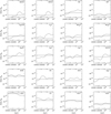 |
Fig. 10 Comparison between Nautilus predictions obtained using our updated chemical network and the abundances observed toward TMC 1 (CP; see Table 4). Gray regions indicate the observed values. We assume an uncertainty of a factor of 2 in the measured abundances. The physical and chemical conditions used in our calculations are: nH = 3 × 104 cm−3, Tk = 10 K, AV = 20 mag, |

Acknowledgements
The research leading to these results has received funding from MICIN (Spain) under grant PID2021-122549NB-C21 and from the European Union’s Horizon 2020 research and innovation program under the Marie Sklodowska-Curie grant agreement No 894321. N.B. is grateful for support from the Polish National Agency for Academic Exchange (NAWA) Grant and also acknowledges TUBITAK’s 2219-Program by scholarship no. 1059B192200348. P.S.Z. is grateful to National Science Centre of Poland for funding the project No 2019/34/E/ST4/00407. A.F. and P.R.M. are grateful to Spanish MICIN for funding under grant PID2019-106235GB-I00. J.R.G. thanks the Spanish MCINN for funding support under grant PID2019-106110GB-I00. J.E.P. was supported by the Max-Planck Society. D.N.A. acknowledges funding support from Fundación Ramón Areces through its international postdoc grant program. R.L.G. would like to thank the “Physique Chimie du Milieu Interstellaire” (PCMI) programs of CNRS/INSU for their financial supports.
References
- Adande, G. R., Halfen, D. T., Ziurys, L. M., Quan, D., & Herbst, E. 2010, ApJ, 725, 561 [NASA ADS] [CrossRef] [Google Scholar]
- Aguado, A., & Paniagua, M. 1992, J. Chem. Phys., 96, 1265 [NASA ADS] [CrossRef] [Google Scholar]
- Aguado, A., Tablero, C., & Paniagua, M. 1998, Comput. Phys. Commun., 108, 259 [NASA ADS] [CrossRef] [Google Scholar]
- Agúndez, M., & Wakelam, V. 2013, Chem. Rev., 113, 8710 [Google Scholar]
- Alexander, M. H. 1998, J. Chem. Phys., 108, 4467 [NASA ADS] [CrossRef] [Google Scholar]
- Atahan, S., Kłos, J., Zuchowski, P. S., & Alexander, M. H. 2006, Phys. Chem. Chem. Phys., 8, 4420 [NASA ADS] [CrossRef] [Google Scholar]
- Boogert, A. C. A., Schutte, W. A., Helmich, F. P., Tielens, A. G. G. M., & Wooden, D. H. 1997, A&A, 317, 929 [NASA ADS] [Google Scholar]
- Bulut, N., Roncero, O., Aguado, A., et al. 2021, A&A, 646, A5 [NASA ADS] [CrossRef] [EDP Sciences] [Google Scholar]
- Cazaux, S., Carrascosa, H., Muñoz Caro, G. M., et al. 2022, A&A, 657, A100 [NASA ADS] [CrossRef] [EDP Sciences] [Google Scholar]
- Cernicharo, J., Lefloch, B., Agúndez, M., et al. 2018, ApJ, 853, L22 [CrossRef] [Google Scholar]
- Cernicharo, J., Cabezas, C., Endo, Y., et al. 2021a, A&A, 646, A3 [Google Scholar]
- Cernicharo, J., Cabezas, C., Endo, Y., et al. 2021b, A&A, 650, A14 [Google Scholar]
- Davidson, E. R. 1975, J. Comp. Phys., 17, 87 [NASA ADS] [CrossRef] [Google Scholar]
- Denis-Alpizar, O., Quintas-Sánchez, E., & Dawes, R. 2022, MNRAS, 512, 5546 [NASA ADS] [CrossRef] [Google Scholar]
- Dubernet, M. L., & Hutson, J. 1994, J. Chem. Phys., 101, 1939 [NASA ADS] [CrossRef] [Google Scholar]
- Dunning, T. H., Jr. 1989, J. Chem. Phys., 90, 1007 [NASA ADS] [CrossRef] [Google Scholar]
- Esplugues, G., Fuente, A., Navarro-Almaida, D., et al. 2022, A&A, 662, A52 [NASA ADS] [CrossRef] [EDP Sciences] [Google Scholar]
- Ferrante, R. F., Moore, M. H., Spiliotis, M. M., & Hudson, R. L. 2008, ApJ, 684, 1210 [NASA ADS] [CrossRef] [Google Scholar]
- Flower, D. R., & Launay, J. M. 1977, J. Phys. B: At. Mol. Phys., 10, 3673 [NASA ADS] [CrossRef] [Google Scholar]
- Fuente, A., Cernicharo, J., Roueff, E., et al. 2016, A&A, 593, A94 [NASA ADS] [CrossRef] [EDP Sciences] [Google Scholar]
- Fuente, A., Navarro, D. G., Caselli, P., et al. 2019, A&A, 624, A105 [NASA ADS] [CrossRef] [EDP Sciences] [Google Scholar]
- Fuente, A., Rivière-Marichalar, P., Beitia-Antero, L., et al. 2023, A&A, 670, A114 [NASA ADS] [CrossRef] [EDP Sciences] [Google Scholar]
- Fuentetaja, R., Agúndez, M., Cabezas, C., et al. 2022, A&A, 667, A4 [Google Scholar]
- Garrod, R. T., Wakelam, V., & Herbst, E. 2007, A&A, 467, 1103 [NASA ADS] [CrossRef] [EDP Sciences] [Google Scholar]
- Georgievskii, Y., & Klippenstein, S. J. 2005, J. Chem. Phys., 122, 194103 [Google Scholar]
- Gerner, T., Beuther, H., Semenov, D., et al. 2014, A&A, 563, A97 [NASA ADS] [CrossRef] [EDP Sciences] [Google Scholar]
- Goicoechea, J. R., & Cuadrado, S. 2021, A&A, 647, A7 [NASA ADS] [CrossRef] [EDP Sciences] [Google Scholar]
- Goicoechea, J. R., Pety, J., Gerin, M., et al. 2006, A&A, 456, 565 [NASA ADS] [CrossRef] [EDP Sciences] [Google Scholar]
- Goicoechea, J. R., Aguado, A., Cuadrado, S., et al. 2021, A&A, 647, A10 [EDP Sciences] [Google Scholar]
- Gómez-Carrasco, S., Félix-González, D., Aguado, A., & Roncero, O. 2022, J. Chem. Phys., 157, 084301 [CrossRef] [Google Scholar]
- Gratier, P., Majumdar, L., Ohishi, M., et al. 2016, ApJS, 225, 25 [Google Scholar]
- Grozdanov, T. P., & Solov’ev, E. A. 1982, J. Phys. B, 15, 1195 [NASA ADS] [CrossRef] [Google Scholar]
- Gu, X., Guo, Y., Zhang, F., Mebel, A. M., & Kaiser, R. I. 2006, Faraday Discuss., 133, 245 [NASA ADS] [CrossRef] [Google Scholar]
- Hapka, M., Zuchowski, P. S., Szczęśniak, M. M., & Chałasiński, G. 2012, J. Chem. Phys., 137, 164104 [NASA ADS] [CrossRef] [Google Scholar]
- Hasegawa, T. I., & Herbst, E. 1993, MNRAS, 261, 83 [NASA ADS] [CrossRef] [Google Scholar]
- Herzberg, G. 1950, Molecular Spectra and Molecular Structure. I. Spectra of Diatomic Molecules (New Yok: van Nostrand Reinhold Co.) [Google Scholar]
- Hily-Blant, P., des Forêts, G. P., Faure, A., & Lique, F. 2022, A&A, 658, A168 [NASA ADS] [CrossRef] [EDP Sciences] [Google Scholar]
- Huber, K. P., & Herzberg, G. 1979, Molecular Spectra and Molecular Structure, IV. Constants of Diatomic Molecules (Toronto: Van Nostrand) [CrossRef] [Google Scholar]
- Jiménez-Escobar, A., & Muñoz Caro, G. M. 2011, A&A, 536, A91 [Google Scholar]
- Jiménez-Escobar, A., Muñoz Caro, G. M., & Chen, Y. J. 2014, MNRAS, 443, 343 [Google Scholar]
- Karplus, M., Porter, R. N., & Sharma, R. D. 1965, J. Chem. Phys., 43, 3259 [NASA ADS] [CrossRef] [Google Scholar]
- Kendall, R. A., Dunning, T. H., & Harrison, R. J. 1992, J. Chem. Phys., 96, 6796 [NASA ADS] [CrossRef] [Google Scholar]
- Klos, J., Szczesniak, M. M., & Chalasinski, G. 2004, Int. Rev. Phys. Chem., 23, 541 [NASA ADS] [CrossRef] [Google Scholar]
- Konings, M., Desrousseaux, B., Lique, F., & Loreau, J. 2021, J. Chem. Phys., 155, 104302 [NASA ADS] [CrossRef] [Google Scholar]
- Laas, J. C., & Caselli, P. 2019, A&A, 624, A108 [NASA ADS] [CrossRef] [EDP Sciences] [Google Scholar]
- Lucas, R., & Liszt, H. S. 2002, A&A, 384, 1054 [NASA ADS] [CrossRef] [EDP Sciences] [Google Scholar]
- McClure, M. K., Rocha, W. R. M., Pontoppidan, K. M., et al. 2023, Nat. Astron., 7, 431 [NASA ADS] [CrossRef] [Google Scholar]
- Minissale, M., Dulieu, F., Cazaux, S., & Hocuk, S. 2016, A&A, 585, A24 [NASA ADS] [CrossRef] [EDP Sciences] [Google Scholar]
- Nagy, T., & Lendvay, G. 2017, J. Phys. Chem. Lett., 8, 4621 [Google Scholar]
- Navarro-Almaida, D., Le Gal, R., Fuente, A., et al. 2020, A&A, 637, A39 [NASA ADS] [CrossRef] [EDP Sciences] [Google Scholar]
- Navarro-Almaida, D., Bop, C. T., Lique, F., et al. 2023, A&A, 670, A110 [NASA ADS] [CrossRef] [EDP Sciences] [Google Scholar]
- Ocaña, A. J., Jiménez, E., Ballesteros, B., et al. 2017, ApJ, 850, 28 [CrossRef] [Google Scholar]
- Palumbo, M. E., Tielens, A. G. G. M., & Tokunaga, A. T. 1995, ApJ, 449, 674 [NASA ADS] [CrossRef] [Google Scholar]
- Palumbo, M. E., Geballe, T. R., & Tielens, A. G. G. M. 1997, ApJ, 479, 839 [NASA ADS] [CrossRef] [Google Scholar]
- Páramo, A., Canosa, A., Le Picard, S. D., & Sims, I. R. 2008, J. Phys. Chem. A, 112, 9591 [Google Scholar]
- Qu, C., & Bowman, J. M. 2016, J. Phys. Chem. A, 120, 4988 [NASA ADS] [CrossRef] [Google Scholar]
- Quack, M., & Troe, J. 1974, Ber. Bunsenges. Phys. Chem, 78, 240 [CrossRef] [Google Scholar]
- Reddy, R. R., Nazeer Ahammed, Y., Rama Gopal, K., & Baba Basha, D. 2003, Astrophys. Space Sci., 286, 419 [NASA ADS] [CrossRef] [Google Scholar]
- Riaplov, E., Wyss, M., Maier, J. P., et al. 2003, J. Mol. Spectrosc., 222, 15 [NASA ADS] [CrossRef] [Google Scholar]
- Rivière-Marichalar, P., Fuente, A., Goicoechea, J. R., et al. 2019, A&A, 628, A16 [Google Scholar]
- Rodríguez-Baras, M., Fuente, A., Riviére-Marichalar, P., et al. 2021, A&A, 648, A120 [NASA ADS] [CrossRef] [EDP Sciences] [Google Scholar]
- Roncero, O., Zanchet, A., & Aguado, A. 2018, Phys. Chem. Chem. Phys., 20, 25951 [NASA ADS] [CrossRef] [Google Scholar]
- Ruaud, M., Wakelam, V., & Hersant, F. 2016, MNRAS, 459, 3756 [Google Scholar]
- Saito, S., Kawaguchi, K., Yamamoto, S., et al. 1987, ApJ, 317, L115 [NASA ADS] [CrossRef] [Google Scholar]
- Sanz-Sanz, C., Aguado, A., Roncero, O., & Naumkin, F. 2015, J. Chem. Phys., 143, 234303 [NASA ADS] [CrossRef] [Google Scholar]
- Senekowitsch, J., Carter, S., Rosmus, P., & Werner, H.-J. 1990, Chem. Phys., 147, 281 [NASA ADS] [CrossRef] [Google Scholar]
- Shingledecker, C. N., Lambers, T., Laas, J. C., et al. 2020, ApJ, 888, 52 [NASA ADS] [CrossRef] [Google Scholar]
- Simon, R., Stutzki, J., Sternberg, A., & Winnewisser, G. 1997, A&A, 327, L9 [NASA ADS] [Google Scholar]
- Song, Y.-Z., Zhang, L.-L., Gao, S.-B., & Meng, Q.-T. 2016, Scientific Rep., 6, 37734 [NASA ADS] [CrossRef] [Google Scholar]
- Spezzano, S., Fuente, A., Caselli, P., et al. 2022, A&A, 657, A10 [NASA ADS] [CrossRef] [EDP Sciences] [Google Scholar]
- Sternberg, A., & Dalgarno, A. 1995, ApJS, 99, 565 [NASA ADS] [CrossRef] [Google Scholar]
- Stoecklin, T., Halvick, P., & Rayez, J. C. 1988, J. Mol. Struct. (Theochem), 163, 267 [CrossRef] [Google Scholar]
- Stoecklin, T., Rayez, J. C., & Duguay, B. 1990a, Chem. Phys., 148, 381 [NASA ADS] [CrossRef] [Google Scholar]
- Stoecklin, T., Rayez, J. C., & Duguay, B. 1990b, Chem. Phys., 148, 399 [NASA ADS] [CrossRef] [Google Scholar]
- Tarroni, R., Carter, S., & Handy, N. C. 2007, Mol. Phys., 105, 1129 [NASA ADS] [CrossRef] [Google Scholar]
- Vastel, C., Quénard, D., Le Gal, R., et al. 2018, MNRAS, 478, 5514 [Google Scholar]
- Vidal, T. H. G., Loison, J.-C., Jaziri, A. Y., et al. 2017, MNRAS, 469, 435 [Google Scholar]
- Visser, B., Beck, M., Bornhauser, P., et al. 2019, Mol. Phys., 117, 1645 [NASA ADS] [CrossRef] [Google Scholar]
- Voronin, A. I. 2004, Chem. Phys., 297, 49 [NASA ADS] [CrossRef] [Google Scholar]
- Wakelam, V., Dartois, E., Chabot, M., et al. 2021, A&A, 652, A63 [NASA ADS] [CrossRef] [EDP Sciences] [Google Scholar]
- Werner, H. J., & Knowles, P. J. 1988a, J. Chem. Phys., 89, 5803 [NASA ADS] [CrossRef] [Google Scholar]
- Werner, H. J., & Knowles, P. J. 1988b, Chem. Phys. Lett., 145, 514 [NASA ADS] [CrossRef] [Google Scholar]
- Werner, H. J., Knowles, P. J., Knizia, G., Manby, F. R., & Schütz, M. 2012, WIREs Comput. Mol. Sci., 2, 242 [CrossRef] [Google Scholar]
- Woon, D. E., & Herbst, E. 2009, ApJS, 185, 273 [Google Scholar]
- Zanchet, A., Roncero, O., González-Lezana, T., et al. 2009, J. Phys. Chem. A, 113, 14488 [CrossRef] [PubMed] [Google Scholar]
- Zanchet, A., Roncero, O., & Bulut, N. 2016, Phys. Chem. Chem. Phys., 18, 11391 [NASA ADS] [CrossRef] [Google Scholar]
- Zanchet, A., del Mazo, P., Aguado, A., et al. 2018, PCCP, 20, 5415 [NASA ADS] [CrossRef] [Google Scholar]
- Zeimen, W. B., Klos, J., Groenenboom, G. C., & van der Avoird, A. 2003, J. Chem. Phys., 118, 7340 [NASA ADS] [CrossRef] [Google Scholar]
- Zhang, L. L., Song, Y. Z., Gao, S. B., & Meng, Q. T. 2018, J. Phys. Chem. A, 122, 4390 [NASA ADS] [CrossRef] [Google Scholar]
All Tables
Parameters used to fit the total reaction rates calculated for CH+S and C2 + S, according to the expression K(T) = A(T/300)Be−C/T
All Figures
|
Fig. 1 CASSCF energies along the reaction coordinate defined as the RCS-RCH distance difference. The energies shown here are obtained for an angle γSCH = 179.9° for the doublet (bottom panel) and quartet (top panel) states for the CH + S → CS + H reaction. Here, we consider five A′ and four A″ electronic states. |
| In the text | |
|
Fig. 2 MRCI+Q energies along the reaction coordinate defined as the RCS-RCH distance difference. The energies shown here are obtained for an angle γSCH = 179.9° for the doublet (bottom panel) and quartet (top panel) states, for the CH + S → CS + H reaction. Three A′ and three A″ electronic states are considered in each case. |
| In the text | |
|
Fig. 3 Angular dependence of the long-range interaction between CH and S in the three lower electronic states. Points are the CASSCF(aV5Z) energies (in cm−1) as a function of the Jacobi angle 9 (defined in the text) for rCH = 1.1199 Å and R = 10, 15, 20 and 30 Å, as indicated in each panel, for the 12A″, 12A′, and 22A″ states. Lines correspond to the long-range analytical fit of Eq. (2) taken from Zeimen et al. (2003). |
| In the text | |
|
Fig. 4 Contour plots of the analytical potential energy surfaces fitted to ab initio points, corresponding to the reactant channel for RCH = 1.1199 Å (bottom panel) and to the products channel for RCS = 1.568 Å (top panel). Energies are in eV. For the products, the energies are shifted by 3.526 eV, so that their point of zero energy corresponds to the CS(req) at an infinite distance from H. The contours correspond to 0 and ± 1 meV in order to show the dependence of the potential at long distances. The units of the color box are eV. |
| In the text | |
|
Fig. 5 CH+S → CS + H reaction probabilities versus collision energy for J = 0 in the 1 2A′ electronic state using quantum wave packet and quasi-classical trajectory methods. |
| In the text | |
|
Fig. 6 Vibrational-selected rate constant for the CH(X2Π,v = 0) + S(3P) → CS(X1Σ) + H reaction, obtained here according to Eq. (6). |
| In the text | |
|
Fig. 7 CASSCF/aVTZ optimized reaction paths for the conversion between C2+S and CS+C, which occurs on several potential energy surfaces of CCS. The reaction coordinate is defined as RCS−RCC, while the valence angle, γCCS, was held fixed at 179.9° in the geometry optimizations. Five A″ and four A′ electronic states of CCS were considered for each multiplicity: triplet (bottom panel), singlet (middle panel), and quintet (top panel). |
| In the text | |
|
Fig. 8 Optimized reaction paths for |
| In the text | |
|
Fig. 9 Reactive rate constant for the C2 + S → CS + S collisions obtained with the present AS method and compared to that available in the KIDA database from Vidal et al. (2017). |
| In the text | |
|
Fig. 10 Comparison between Nautilus predictions obtained using our updated chemical network and the abundances observed toward TMC 1 (CP; see Table 4). Gray regions indicate the observed values. We assume an uncertainty of a factor of 2 in the measured abundances. The physical and chemical conditions used in our calculations are: nH = 3 × 104 cm−3, Tk = 10 K, AV = 20 mag, |
| In the text | |
Current usage metrics show cumulative count of Article Views (full-text article views including HTML views, PDF and ePub downloads, according to the available data) and Abstracts Views on Vision4Press platform.
Data correspond to usage on the plateform after 2015. The current usage metrics is available 48-96 hours after online publication and is updated daily on week days.
Initial download of the metrics may take a while.