| Issue |
A&A
Volume 677, September 2023
Solar Orbiter First Results (Nominal Mission Phase)
|
|
|---|---|---|
| Article Number | A25 | |
| Number of page(s) | 16 | |
| Section | The Sun and the Heliosphere | |
| DOI | https://doi.org/10.1051/0004-6361/202345859 | |
| Published online | 31 August 2023 | |
Stereoscopic disambiguation of vector magnetograms: First applications to SO/PHI-HRT data
1
Max-Planck-Institut für Sonnensystemforschung, Justus-von-Liebig-Weg 3, 37077 Göttingen, Germany
e-mail: This email address is being protected from spambots. You need JavaScript enabled to view it.
; This email address is being protected from spambots. You need JavaScript enabled to view it.
2
Instituto de Astrofísica de Andalucía (IAA-CSIC), Apartado de Correos 3004, 18080 Granada, Spain
e-mail: This email address is being protected from spambots. You need JavaScript enabled to view it.
3
Sorbonne Université, École polytechnique, Institut Polytechnique de Paris, Université Paris Saclay, Observatoire de Paris-PSL, CNRS, Laboratoire de Physique des Plasmas (LPP), 75005 Paris, France
4
Université Paris-Saclay, CNRS, Institut d’Astrophysique Spatiale, 91405 Orsay, France
5
Instituto Nacional de Técnica Aeroespacial, Carretera de Ajalvir, km 4, 28850 Torrejón de Ardoz, Spain
6
Universitat de València, Catedrático José Beltrán 2, 46980 Paterna-Valencia, Spain
7
Institut für Datentechnik und Kommunikationsnetze der TU Braunschweig, Hans-Sommer-Str. 66, 38106 Braunschweig, Germany
8
University of Barcelona, Department of Electronics, Carrer de Martí i Franquès, 1 – 11, 08028 Barcelona, Spain
9
Instituto Universitario “Ignacio da Riva”, Universidad Politécnica de Madrid, IDR/UPM, Plaza Cardenal Cisneros 3, 28040 Madrid, Spain
10
Leibniz-Institut für Sonnenphysik, Schöneckstr. 6, 79104 Freiburg, Germany
11
Institut für Astrophysik, Georg-August-Universität Göttingen, Friedrich-Hund-Platz 1, 37077 Göttingen, Germany
Received:
7
January
2023
Accepted:
9
July
2023
Abstract
Contact. Spectropolarimetric reconstructions of the photospheric vector magnetic field are intrinsically limited by the 180° ambiguity in the orientation of the transverse component. So far, the removal of such an ambiguity has required assumptions about the properties of the photospheric field, which makes disambiguation methods model-dependent.
Aims. The successful launch and operation of Solar Orbiter have made the removal of the 180° ambiguity possible solely using observations of the same location on the Sun obtained from two different vantage points.
Methods. The basic idea is that the unambiguous line-of-sight component of the field measured from one vantage point will generally have a nonzero projection on the ambiguous transverse component measured by the second telescope, thereby determining the “true” orientation of the transverse field. Such an idea was developed and implemented as part of the stereoscopic disambiguation method (SDM), which was recently tested using numerical simulations.
Results. In this work we present a first application of the SDM to data obtained by the High Resolution Telescope (HRT) on board Solar Orbiter during the March 2022 campaign, when the angle with Earth was 27 degrees. The method was successfully applied to remove the ambiguity in the transverse component of the vector magnetogram solely using observations (from HRT and from the Helioseismic and Magnetic Imager) for the first time.
Conclusions. The SDM is proven to provide observation-only disambiguated vector magnetograms that are spatially homogeneous and consistent. A discussion on the sources of error that may limit the accuracy of the method, and strategies to remove them in future applications, is also presented.
Key words: Sun: magnetic fields / Sun: photosphere / methods: observational
© The Authors 2023
 Open Access article, published by EDP Sciences, under the terms of the Creative Commons Attribution License (https://creativecommons.org/licenses/by/4.0), which permits unrestricted use, distribution, and reproduction in any medium, provided the original work is properly cited.
This article is published in open access under the Subscribe to Open model.
Open access funding provided by Max Planck Society.
1. Introduction
The solar photospheric magnetic field can be inferred from spectropolarimetric observations by parametrically matching the measured Stokes spectra with synthetic profiles based on radiative transfer in atmospheric models (see, e.g., Lites 2000). Such a technique (called inversion) can only provide a partial knowledge of the vector field, namely the amplitude and orientation of the field component along the line of sight (LoS) of the observer and the amplitude and direction of the field component perpendicular to the LoS. However, no information is provided about the orientation along the transverse direction of the field, resulting in an ambiguity of the transverse component: two orientations of the transverse component that differ by 180° are indistinguishable from each other. Such an ambiguity is due to the invariance of the Stokes vector to a 180° rotation of the reference system about the LoS axis. Therefore, the 180° ambiguity in the orientation of the transverse field component is an intrinsic limitation of remote sensing that cannot be eliminated by improving spectropolarimetric measurements. On the other hand, solving the 180° ambiguity (disambiguation) corresponds to the determination of the sign of the transverse component in each pixel of the image plane, and it is therefore a parity problem (Semel & Skumanich 1998).
The importance of a correct disambiguation of vector magnetograms can hardly be overestimated. Besides its implication for a proper description of the evolution of the photospheric magnetic field, the orientation of the transverse component enters the computation of the electric currents that are injected into the upper layers of the solar atmosphere. It is only after disambiguation that the observed magnetic field components can be re-projected in the physical radial, toroidal, and poloidal components (Gary & Hagyard 1990; Sun 2013) that are used to compute physically relevant quantities such as radial currents. In turn, such currents are the origin of the free magnetic energy that powers coronal activity (see, e.g., Forbes et al. 2006; Aulanier et al. 2013), from flares to coronal mass ejections, contributing to coronal heating as well as to the variability of the heliospheric environment.
Several empirical methods propose solutions for removing the 180° ambiguity (see Metcalf et al. 2006 for a review and Leka et al. 2009 for additional comparisons). A common limitation of all traditional disambiguation methods is that, in order to compensate for the incomplete information about the transverse magnetic field, they must necessarily rely on assumptions in order to constrain its orientation. Such assumptions may vary from simply choosing the orientation of the transverse field that is closer to the corresponding potential field, to more complex criteria that involve minimizing a weighted combination of vertical electric currents and the divergence of the magnetic field. Typically, such criteria are formulated as a minimization problem, and Table 1 in Leka et al. (2009) lists the quantity to be minimized for several methods. However, as reasonable as they can be, such simplifying assumptions might not always be satisfied, especially in highly complex magnetic field regions that are often the source of space-weather-relevant flare events.
A new possibility for the solution of the 180° ambiguity is offered by the successful launch and operation of Solar Orbiter (Müller 2020; Zouganelis et al. 2020) and its onboard magnetograph, the Polarimetric and Helioseismic Imager (SO/PHI; Solanki et al. 2020). The orbit of Solar Orbiter allows for remote-sensing observations from different vantage points away from the Sun-Earth line. The combination of information on the magnetic field orientation from different viewpoints of the same area on the Sun can now be used to remove the ambiguity observationally (Solanki et al. 2015; Rouillard et al. 2020).
Regardless of the employed method, either single-view or stereoscopic, disambiguation is a step that is affected by the accuracy of the input information. The optical quality of the observations, the limitations and accuracy of the employed inversion technique used to deduce the magnetic vector from spectropolarimetric data, and the accuracy of any geometrical transformation that may be needed for the application of the chosen disambiguation method are all factors that can influence the success of the disambiguation. Such factors should be regarded as influencing, but not being intrinsically part of, the disambiguation method. As mentioned above, single-view methods require additional hypotheses to remove the ambiguity but have the advantage of dealing with such problems for one instrument only. On the other hand, any stereoscopic method is confronted with the additional complication of bringing together information from two different instruments, which prominently entails differences in calibrations, resolution, and (generally) inversion techniques, in addition to requiring a sensitive geometrical procedure for combining views from different vantage points.
Valori et al. (2022, hereafter Paper I), introduced the stereoscopic disambiguation method (SDM), which solves the 180° ambiguity by combining information from two vantage points. Unlike traditional, single-viewpoint methods, the SDM solves the ambiguity based on observations only, without any assumption about the magnetic field. Paper I also used numerically simulated vector magnetograms to show that the SDM can remove the ambiguity with great accuracy over a large range of stereoscopic angles.
In this article we present the very first application of the SDM to real observations. We use co-temporal observations from the SO/PHI High Resolution Telescope (SO/PHI-HRT; Gandorfer et al. 2018) and from the Helioseismic and Magnetic Imager (HMI; Scherrer et al. 2012; Schou et al. 2012) on board the Solar Dynamics Observatory (SDO; Pesnell et al. 2012).
The SDM and its application are described in Sect. 2. In Sect. 3 we provide details of the data sets used in the presented tests, both from SO/PHI-HRT and from two distinct SDO/HMI-data product series. The results of two SDM disambiguations of the same SO/PHI-HRT vector magnetogram but using the two SDO/HMI data series are presented in Sects. 4 and 5. In Sect. 6 we discuss possible sources of error and future improvements of the SDM, and Sect. 7 summarizes our conclusions.
2. The stereoscopic disambiguation method
The stereoscopic disambiguation of vector magnetograms can be split into two independent steps: first, the solution of the geometrical problem of relating the components of a same vector magnetic field as seen from two different vantage points (Sect. 2.1). Second, the practical application of the method to real observations (Sect. 2.2) and its numerical implementation (Sect. 2.3).
2.1. SDM: The geometrical problem
Paper I derives the equations to determine the sign ζ = ±1 of the transverse component in each pixel of the image planes of two telescopes. For each telescope, for example for the telescope A, a SDM reference system SA is defined by three unit-vectors: the direction of the LoS ( ), the common normal (
 ) to the plane through the telescopes A and B and the center of the Sun, and their normal vector (
 ; see Fig. 1 in Paper I). We note the change in notation
  with respect to Paper I, adopted here to avoid any possible confusion with the component of the field normal to the solar surface). In
  the magnetic field, B, is written as
 (1)
(1)
where  is the (signed) LoS component and
 (2)
(2)
with the polar angle αA defined in [0, π] and  is the (positive-defined) amplitude of the transverse component. Analogous expressions hold for the reference system
  of the telescope B, namely
 (3)
(3)
with
 (4)
(4)
In practice, SA (respectively, SB) is a rotation of the detector reference system by an angle θA (respectively, θB) around the LoS such that the detector y direction is parallel to  . Since by construction
  is the same for SA and SB, and since both αA and αB are restricted between 0 and π, it follows that the
  components on SA and SB are identical regardless of the ambiguity, namely
  (and the sign function ζ is the same in Eq. (1) and Eq. (3); see in particular Eq. (8) in Paper I for a proof). The property that
  is used in Sect. 4.2.2 as a consistency criteria for the application of the SDM.
Using the above representation, Paper I shows that the sign of the transverse component, ζ, is given by either of the two geometrically equivalent formulae,
 (5)
(5)
 (6)
(6)
where γ is the separation angle between the two telescopes A and B, defined as counterclockwise around  from the direction of telescope A.
In Eq. (5) the Bw components of both telescopes A and B appear, while in Eq. (6) only  does. In other words, Eq. (6) can be applied to disambiguate the transverse component on telescope A even if only the LoS component on telescope B is available (see Sect. 5 for an application of this particular case).
2.2. SDM: Application to observations
Equations (5) and (6) can be applied in several ways to data from SO/PHI-HRT and SDO/HMI. First, one can disambiguate A magnetograms using information from B (the “direct” case of Sect 3.3.1 in Paper I), or vice versa (the “reverse” case). Second, the sign ζ of the transverse component can be determined by either Eq. (5) or Eq. (6), or a combination of the two (see Sect. 3.3.2 in Paper I in particular). Finally, different SDO/HMI data series can be used as input for the SDM.
In this paper we consider the disambiguation of the SO/PHI-HRT data set using two different SDO/HMI series (Sect. 3.2). In the terminology of Paper I, this case corresponds to the reverse application of the SDM with the associations A = SO/PHI-HRT and B = SDO/HMI. In this first application we do not consider disambiguation of SDO/HMI using SO/PHI-HRT because of the unfavorable position of the target active region (AR) on the solar disk (see Sect. 3).
2.3. SDM: Numerical implementation
In order to use Eqs. (5) and (6) in real applications, the observed vector magnetic field from each telescope must be first transformed from the image plane to the corresponding SDM reference system. In this section we provide an example of the SDM workflow for the reverse applications presented in the following sections. The SDM software is developed using the SolarSoft suite of programs (Freeland & Handy 2012). The following steps are performed to apply the SDM to a given SO/PHI-HRT data set:
SDO/HMI data selection (1). The SDO/HMI magnetogram should be chosen as the one closest in time to the considered SO/PHI-HRT observation. However, due to the generally smaller distance of Solar Orbiter from the Sun, the difference in light travel-time between Solar Orbiter and SDO must be considered. Hence, the selected SDO/HMI data set is chosen as the closest in time (as specified by the T_OBS FITS keyword; see Couvidat et al. 2016) to the time at which the light measured by SO/PHI-HRT would have reached Earth. The latter is readily provided by the FITS keyword DATE_EAR in the FITS header of the SO/PHI-HRT data set. No further time adjustments is considered at this stage.
Image co-registration (2). This step is crucial for the application of the SDM, which intrinsically requires the alignment between images to have subpixel accuracy. Currently, the World Coordinate System (WCS; Thompson 2006) keywords in SO/PHI-HRT do not match the SDO/HMI ones to such a degree of accuracy; therefore, a co-registration step is unavoidable. The co-registration is performed using the field strength as comparison when possible, which is ideally independent of the viewing angle, unless only Blos is available (as in Sect. 5).
The SDO/HMI image is first remapped onto the SO/PHI-HRT detector frame, then a sub-domain of co-registration is chosen. The remapping includes the (bi-linear) interpolation of the SDO/HMI image onto the SO/PHI-HRT uniform grid. The co-registration technique is a simple but fast and accurate Fourier matching technique that provides the co-registration shifts to apply to the SO/PHI-HRT reference pixel identified by the WCS keywords CRPIX1 and CRPIX2. The remapping/co-registration steps are repeated, each time using the newly updated SO/PHI-HRT WCS keywords, until convergence is reached to the desired precision (to better than 1/100th of a pixel, in the application here). We verified that, for the SO/PHI-HRT data set considered here, the correction to the WCS keyword CROTA, representing the rotation angle of the detector with respect to solar north, is negligible. The co-registration procedure is in principle independent of the sub-domain where the SDM is applied, although here we use the same field of view (FoV) for both.
Remapping of the SDO/HMI Cartesian magnetic field components on the SO/PHI-HRT detector frame (3). This step uses the co-registered SO/PHI-HRT WCS information as updated in step 2. The remapping entails a (bi-linear) interpolation of the SDO/HMI magnetogram (upscaling SDO/HMI to the SO/PHI-HRT resolution in the cases presented here).
Computation of the separation angle, γ, and the SDM rotation angles θA and θB (4). These angles are directly computed from the observer Carrington coordinates as included in the FITS headers of the considered SO/PHI-HRT and SDO/HMI data set.
Re-projection of the SO/PHI-HRT and SDO/HMI vector magnetic fields on the SDM reference systems, SA and SB respectively (5). This step produces the representation of the vector magnetic field according to Eqs. (1, 3), with the azimuth of both fields renormalized to be within [0, π].
Application of the relevant SDM equation (either Eq. (5) or Eq. (6)) to compute the sign function, ζ (6). In order to constrain ζ to the nominal ±1 values, we then build a parity map by taking the sign of ζ (see also Sect. 4.2.1).
Disambiguation (7). The parity map is then applied to the SO/PHI-HRT transverse component to remove the ambiguity. Once disambiguated, the SO/PHI-HRT field is re-projected back to the detector reference system for ease of comparison.
3. Observations and data preparation
We considered the observation of NOAA AR12965 taken by SO/PHI-HRT and SDO/HMI on March 17, 2022, when Solar Orbiter was at 0.38 AU from the Sun and the separation angle with SDO was γ = 26.53°. The Carrington longitude and latitude of the target AR were (271.5° ,22.5° ), respectively. Figure 1 shows the LoS magnetic field (Blos) of the chosen data sets on the full image planes of the two telescopes. The rationale behind this choice amongst those available in the first months of the science mission phase of Solar Orbiter is that it contains a well-formed AR within the FoV, and that observations are taken when the two telescopes are well within the range of stereoscopic angles, that is, far enough from both quadrature and inferior conjunction (see also Sect. 4.4 in Paper I). The AR contains two compact sunspots of positive polarities (see also Fig. 2) close to each other, and a more dispersed, following negative-polarity region. The two positive sunspots in the AR are of particular interest for this first application of the SDM because they allow for some qualitative considerations about the expected orientation of the transverse component. The same AR was also studied in Li & Long (2023), where observations from the Extreme Ultraviolet Imager (Rochus et al. 2020) on board Solar Orbiter were exploited to study oscillations in coronal loops.
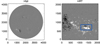 |
Fig. 1. Blos on March 17, 2022, on the image planes of SDO/HMI (left, at 03:46:35.5 UT) and SO/PHI-HRT (right, at 03:44:09 UT). The blue rectangle on the SO/PHI-HRT image shows the sub-domain that is used for co-registration (see step 2 in Sect. 2.3) and SDM application. The images are not rotated, meaning that solar north is approximately down in SDO/HMI (left) and up in SO/PHI-HRT (right). In both panels, axes are in pixels. |
While the above criteria identified the chosen data set as the only suitable one available at the time of writing, it is still not ideal. First, because the AR was relatively close to the limb of SDO/HMI (see the left panel in Fig. 1), it is therefore affected by strong foreshortening effects. Second, the separation angle γ is also not very large, which is expected to adversely impact the accuracy of the method: according to the tests on numerical simulations discussed in Paper I, the SDM accuracy at γ ≊ 27° is close to 100% in smooth field areas (see, e.g., Fig. 10c in Paper I), while it can be significantly lower in quiet-sun regions (see, e.g., Fig. 10e in Paper I, where SDM yields the correct disambiguation in 75% of the pixels in that test). We note the specific combination of γ and spacecraft distance from the Sun presented here are not explicitly included in any of the tests presented in Paper I, so the comparison between numerical tests and application to observations can only be indicative.
3.1. SO/PHI-HRT
On March 17, the SO/PHI-HRT observed the target AR for 30 min with a high-cadence program (the Nanoflare-Solar Orbiter Observation Plan in Zouganelis et al. 2020). The data set used in this work has Data IDentification (DID) number 0243170227 with observation time 03:44 UT. At the distance of 0.38 AU, the SO/PHI-HRT pixel scale at disk center is equal to 137.2 km. The 24 polarization images used to build the Stokes vector were acquired with a fast accumulation mode lasting 60 s.
The spectropolarimetric observations were calibrated, and the inversion of the radiative transfer equation (RTE) followed Sinjan et al. (2022). In short, dark-current and flat-field corrections are first applied. The flat field is preliminary corrected using unsharp masking with a Gaussian amplitude of 69 pixels. Since the SO/PHI-HRT image stabilization system (Volkmer et al. 2012) was not in operation during the acquisition, a co-registration of the polarization images is also applied (see also Calchetti et al. 2023).
After demodulation and cross-talk correction, the RTE inversion is performed using the CMILOS code (Orozco Suárez & Del Toro Iniesta 2007), which assumes a Milne-Eddington atmosphere and employs analytical response functions to build the synthetic profiles that are used in the minimization process. The filling factor is assumed to be unity. A detailed description of the above steps is found in Sinjan et al. (2022). The above constitutes the currently standard version of the SO/PHI-HRT pipeline, and no additional processing was applied to the data. In particular, the employed data have not been reconstructed and aberration-corrected, as described by Kahil et al. (2023; see our Sect. 6.1 for further details).
In addition to the disambiguation using the SDM, we also performed a disambiguation of the same data set using a classical method that, unlike the SDM, only uses data from a single telescope. The disambiguation that we applied, hereafter ME0, is an adaptation of the disambiguation code in the SDO/HMI pipeline (Hoeksema et al. 2014), which, in turn, implements the “minimal energy method” (Metcalf 1994; Metcalf et al. 2006). The parameters used for the ME0 disambiguation are similar to those used in the HMI pipeline, and no particular attempt was made to optimize them. However, the ME0 method requires the definition of a noise mask to determine where to apply annealing. This was built as a linear mask with the corresponding parameters bthresh1 = 300 G and bthresh2 = 400 G, which represent upper levels of noise on the transverse component of the field at disk center and at the limb, respectively.
In order to fix bthresh1,2, the noise level on the SO/PHI-HRT magnetogram is estimated in two ways: first, as the standard deviation of the Gaussian fit of the histogram distribution of transverse field values in quiet Sun areas. Such an estimation results in a noise level on the transverse component equal to 64 G (and of 8.47 G on Blos; see also Sinjan et al. 2023). Second, with a similar method as the above, the noise on the Stokes components are found to be (1.73, 1.27, 1.34)×10−3 for (Q, U, V)/Ic, respectively. Using these values in the magnetographic formulae for classical calibration as given by Eq. (4) in Martínez Pillet (2007), we find a second estimate for the noise on the transverse component equal to 147 G (and 8.89 G on Blos). The employed values for bthresh1 and bthresh2 correspond to approximately three times the average of such noise estimations, for observations at center of disk and limb, respectively.
3.2. SDO/HMI
The SDO/HMI magnetograms used for the SDM application are chosen to match as close as possible the SO/PHI-HRT observation time corrected for the difference in light-travel time (step 1 in Sect. 2.3).
Two SDO/HMI data sets from two different SDO/HMI data product series are considered. The first data set is the SDO/HMI vector magnetogram with the observation date of March 17, 2022, 03:46:35.5 from the hmi.ME_720s_fd10 series (corresponding to the observation time as registered by the FITS keyword T_OBS = 03:47:21 UT). For the considered data sets, the difference in light travel time between Solar Orbiter and SDO is 307.6 s. The hmi.ME_720s_fd10 series provides vector magnetograms (inclination, ambiguous azimuth, and field strength) at a cadence of 720 s resulting from averages of observations taken over 20 min (Hoeksema et al. 2014), and produced by the very fast inversion of the Stokes vector Milne-Eddington code (VFISV; Borrero et al. 2011; Hoeksema et al. 2014). The price to pay for having the vector information is that, due to the averaging procedure, the observation are generally more difficult to match in time with SO/PHI-HRT observations.
The second data set is the SDO/HMI magnetogram obtained on March 17, 2022, at 03:48:28.0 from the 45 s data series, hmi.m_45s. For this data set, T_OBS = 17-Mar-2022 03:48:51 UT. The hmi.m_45s data series provides the LoS magnetic field only but, thanks to its high-cadence, the SDO/HMI observation time can be chosen to be very close to the time of the SO/PHI-HRT data set. The hmi.m_45s data series employs an “MDI-like” inversion method (Couvidat et al. 2012) that is based on a discrete Fourier expansion of the solar neutral iron line, corrected for the SDO/HMI filter transmission profile (Hoeksema et al. 2014; Couvidat et al. 2016). Hoeksema et al. (2014) showed that, in areas where |B|> 300 G, the values obtained by the RTE inversion in the hmi.ME_720s_fd10 series are larger than those obtained by the MDI-like algorithm used for the hmi.m_45s data series (see Fig. 17 in Hoeksema et al. 2014).
In addition to the above, we also considered a data set from the hmi.ME_90s series, which is a series similar to the hmi.ME_720s_fd10 series but with a cadence of 90 s instead of 720 s. Data products for such a series are available on demand, and were not readily available for the relevant date. For this reason, we do not employ the hmi.ME_90s series in this article, although the results from a few ancillary tests made using that series are presented in Sect. 6.
4. SDM disambiguation using the hmi.ME_720s_fd10 series
In this section we present the results of the disambiguation of the SO/PHI-HRT vector magnetogram using the SDM and the hmi.ME_720s_fd10 data series as input (i.e., the reverse case, with A = SO/PHI-HRT and B = SDO/HMI; see Sect. 2.2). First, steps 2 and 3 of the procedure in Sect. 2.3 were performed, using the field strength as the co-registration field. The sub-domain used for co-registration (and SDM application) is the blue rectangle in the right panel of Fig. 1. As a result, the SDO/HMI magnetogram is co-registered with, re-projected onto, and remapped on the SO/PHI-HRT image plane, to which we refer hereafter as the “remapped-SDO/HMI” magnetogram. For the nominal helioprojective coordinates of the reference pixel CRVAL1,2 = (416.36,1281.19), the co-registered reference pixel values are found to be CRPIX1,2 = (1230.72, 983.07). The images co-registration is then the same for the two applications in Sects. 4.1 and 4.4. A qualitative check of the co-registration procedure obtained using the field strength is given by Fig. 2a,b, which show the continuum intensity of the remapped SDO/HMI and SO/PHI-HRT, respectively, with the isolines of the SDO/HMI continuum overlaid on both images. The co-registration of the two data sets is globally very accurate, with a (Pearson) correlation coefficient of the field strength equal to 0.97.
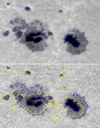 |
Fig. 2. Continuum images on the SO/PHI-HRT image plane of (a) remapped SDO/HMI and (b) SO/PHI-HRT data sets. The continuum intensity is normalized by its median value and shown between 0.5 and 1.2. In both panels, the isocontours of the SDO/HMI continuum intensity at [15.,25.,35.] × 103 DN s−1 (corresponding to [0.37, 0.62, 0.86] in normalized units) are drawn as solid blue lines. In panel b, the 400 G isoline of the SO/PHI-HRT |Blos| is drawn as a solid yellow line. |
In order to quantitatively further describe the co-registration accuracy, we divided the co-registration sub-domain into tiles of 64 × 64 pixels and recomputed the co-registration shifts between the remapped SDO/HMI and the (co-registered) SO/PHI-HRT images in each tile separately, following the same iterative procedure as step 2 in Sect. 2.3. This results in the maps of residual misalignment shown in Fig. 3a,b, which shows that, with few exceptions, all residual shifts are within ±2 pixels. The residual shifts are, however, often of variable magnitude and different sign, even between adjacent tiles. As discussed more extensively in Sect. 6.1, this can likely be attributed to uncorrected aberrations in the employed SO/PHI-HRT data set.
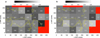 |
Fig. 3. Residual cross-correlation shifts after co-registration, computed in tiles of 64 × 64 pixels, in the x (panel a) and y direction (panel b). The number at the center of each tile is the co-registration shift for that tile, in units of SO/PHI-HRT pixels. Tiles where the cross-correlation procedure did not converge are marked in red. In both panels, the 400 G isoline of the SO/PHI-HRT |Blos| is drawn as a solid yellow line. |
Next, either Eq. (5) or Eq. (6) is applied to remove the ambiguity of the SO/PHI-HRT transverse field.
4.1. First observation-based disambiguation
We first consider the application of Eq. (5). Following steps 3–7 in Sect. 2.3, a parity map is produced that takes in each SO/PHI-HRT pixel the value −1 (respectively, +1) where the transverse component is (respectively, is not) to be reversed. Applying the parity map to the SO/PHI-HRT ambiguous transverse component we obtain the first SDM-disambiguated vector magnetogram, shown in Fig. 4a. On a qualitative level, the SDM disambiguation of the SO/PHI-HRT magnetogram is remarkably successful. In particular, the transverse component has the expected orientation, namely it is pointing radially outward in positive flux concentrations. The transverse component is also smoothly distributed almost everywhere on the main polarities. This is true also for the bottom part of the AR, where projection effects shorten the amplitude of the transverse component considerably. Such properties are remarkable if one recalls that, in order to produce the SDM-disambiguated transverse field, no assumption about the transverse field is made: the disambiguation in Fig. 4 solely results from combining information from two points of view (two telescopes) in each SO/PHI-HRT pixel separately. Localized areas where the orientation of the transverse component is different from that expected are discussed in Sect. 4.2, whereas general accuracy considerations are summarized in Sect. 6.
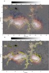 |
Fig. 4. First observation-based SDM-disambiguated vector magnetogram. The SO/PHI-HRT vector magnetogram is disambiguated using SDO/HMI information from the (ambiguous) hmi.ME_720s_fd10 data series and Eq. (5). Panel a: background image representing Blos on the SO/PHI-HRT image plane, saturated at ±1500 G in grayscale; red and blue arrows represent the transverse field at positive and negative Blos, respectively. The 400 G isoline of |Blos| is drawn as a solid yellow line. Panel b: same as panel a but in remapped Stonyhurst coordinates, with the magnetic field re-projected in radial, poloidal, and toroidal components. In this panel, the background image represents the radial component Br saturated at ±1500 G in grayscale, and red and blue arrows represent the horizontal field at positive and negative Br, respectively. The 400 G isoline of |Br| is drawn as a solid yellow line. |
4.2. Disambiguation diagnostic
Besides the overall consistency of the disambiguation in Fig. 4, there are specific locations where the orientation of the transverse component is suspicious. Two such areas follow the polarity inversion line of Blos (PILLoS) in the penumbral areas, highlighted by the orange rectangles at (x, y)≃(180, 170) and (x, y)≃(340, 130) in Fig. 5b. While in most places the blue arrows continue pointing away from the spots, as expected in the crossing of the PILLoS in the penumbra (i.e., where arrows change color from red to blue), at these locations, the blue arrows point in the opposite direction to the red arrows and are seemingly interlaced with them.
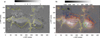 |
Fig. 5. Application of the SDM using the hmi.ME_720s_fd10 series and Eq. (5). Panel a: sign function ζ saturated at ±5. Panel b: corresponding SDM-disambiguated vector magnetogram, with Blos saturated at ±1500 G in grayscale and red and blue arrows representing the transverse field at positive and negative Blos (same as Fig. 4a). The rectangles in panel b indicate the areas of suspicious disambiguations discussed in Sect. 4.2 (black) and Sect. 4.2.1 (orange and green). In both panels, the 400 G isoline of the SO/PHI-HRT |Blos| is drawn as a solid yellow line. |
Another two areas of suspicious disambiguation lie along linear features at (x, y)≃(180, 110) and (x, y)≃(330, 80) (highlighted by black rectangles in Fig. 5b), where the arrows representing the transverse field are left-oriented, opposite in orientation to those right above and below that line but of similar amplitude, and, therefore, arguably pointing in the wrong direction.
The real orientation of the transverse component in Fig. 4 is not known, and a quantitative assessment of the SDM accuracy (as well as of any other method) is not possible in such a case. However, and in contrast to traditional single-view methods, the SDM offers diagnostic tools that help assess at which specific locations the method is likely to be less accurate.
The evaluation of the correctness of the disambiguation is customarily performed writing the field in the “heliographic” (Gary & Hagyard 1990) radial, toroidal, and poloidal components (or, more precisely, in heliocentric spherical coordinates; see Thompson 2006; Sun 2013). In addition, in order to compensate for foreshortening effects, the field is remapped (i.e., interpolated) onto the Stonyhurst coordinates (Thompson 2006). The resulting vector magnetogram in heliographic projection is shown in Fig. 4b. The polarity inversion line, not drawn, is the line separating blue from red arrows. One can clearly see how some of the suspicious areas discussed above affect the re-projected field shown in Fig. 4b. In particular, the black boxes in Fig. 5b correspond to areas (slightly shifted downward by the re-projection) where the radial field is smaller than in their surroundings, yielding darker (but still of positive value) structures in the cores of the spots. Even more remarkably, a true reversal of the radial component can be seen in correspondence of the penumbral area highlighted by the right-orange box in Fig. 5b: here the horizontal field is drawn in blue arrows, meaning that corresponds to negative values of the radial component. Such effects are a clear example of how errors in the disambiguation of the transverse field component can heavily affect all (physically relevant) field components in the local frame. On the other hand, the areas marked by the left-orange and green box in Fig. 5b are not readily recognizable as suspicious in Fig. 4b.
In our identification of suspicious areas, the assumption that the transverse component is smooth across neighboring pixels is implicitly made, which has some similarities with the hypothesis that underlies the ME0 method. However, such an assumption does not enter at any point the derivations of Eqs. (5) and (6). Moreover, in the following we introduce diagnostic quantities that are able to identify exactly such areas as locations of potentially wrong disambiguations regardless of any continuity assumption. Since such diagnostic quantities are defined in the image plane rather than in the heliographic plane, we prefer to discuss them primarily in the former rather than remap them onto the latter, thereby avoiding the loss of the pixel-by-pixel connection to the observed quantities appearing in Eqs. (5) and (6).
4.2.1. The sign function ζ
In principle, the sign function ζ in Eq. (5) (as well as in Eq. (6)) should take only the values ±1. However, since ζ is determined as a combination of field components from different instruments, fluctuations due to noise or any difference in observation time, instrument calibration, RTE inversion, or co-registration would produce departures from the nominal values. Conversely, the departure of Eq. (5) from the nominal ±1 values can be used as a diagnostic metric for the SDM.
The application of Eq. (5) results in the map of ζ that is shown in Fig. 5a, where large departures from the nominal ±1 values show up as black/white pixels, mostly, but not exclusively, in low-field, quiet-sun areas outside the 400 G yellow isoline. Discarding the latter, the most prominent area of errors is around (x, y)≃(280, 80), marked by the green rectangle in Fig. 5b, which was recognized to be an area of low-signal in the SO/PHI-HRT linear polarization yielding difficulties in the inversion.
Other locations where the sign function ζ significantly departs from the nominal values is the PILLoS of Blos, indeed where the orange rectangles in Fig. 5b indicates suspicious disambiguations. At this PILLoS, the transverse field is relatively large. However, the LoS component is not, and may fluctuate due to noise, or difficulties in the inversion from atypical Stokes V profiles (see Solanki & Montavon 1993). Since Blos is the only term at the numerator of Eq. (5), such fluctuations can easily be the origin of the “salt and pepper” large values of ζ found in these areas.
In addition, we notice the roughly horizontal separation line between −1 (bottom) and +1 (top) values across the main polarity concentrations (before disambiguation, all arrows point upward because of αA being restricted to [0; π]). Such a line is not a “special” place in any physical sense: it is ultimately determined by the mutual orientation and locations of the spacecraft (via θA and θB) and the particular distribution of the observed field (via αA). However, the horizontal transition line between ζ = +1 and ζ = −1 is spatially correlated to the linear distribution of suspicious arrows above.
4.2.2. The Bv components
In order to have a more quantitative analysis of the above disambiguation result we exploit the property of the SDM that the Bv component of SO/PHI-HRT and the Bv component of the remapped-SDO/HMI should be identical (see Sect. 2.1). Such a property should be considered a prerequisite for application of the SDM, and pixels where the property is not fulfilled are expected to be more prone to disambiguation errors. On the other hand, it is necessary condition for the application of the SDM that involves only the transverse components, meaning that disambiguation errors that are originated from the LoS components only can still occur even if the two Bv component are identical. Hence, we can use the metric
 (7)
(7)
as a measure of how well the assumptions of the SDM are fulfilled in the practical application. Since Bv is by construction positive, δBv varies between −1 and +1, and takes the value zero where the two components are identical.
We notice that a metric similar to Eq. (7) can be equally constructed using the field strength, |B|, which is also theoretically independent of the point of view. Tests not reported here show, however, that no information that is relevant to the SDM result is really gained in this way: differences in field strength between SO/PHI-HRT and SDO/HMI are relatively small, as documented by Sinjan et al. (2023), and do not discriminate the role of the azimuth in any way.
The relative difference, δBv, is shown in Fig. 6a. Except for purely quiet-sun areas, δBv is indeed found to be close to zero everywhere, which indicates that most of the considered FoV fulfills the requirements for the application of the SDM. However, a remarkable double stripe of opposite δBv unitary values is evident around y ≃ 100. This double-stripe structure in δBv is due to an apparent shift in the vertical direction of the two Bv distributions. The apparent shift is confirmed by the plot of the Bv components in the upper panel of Fig. 6b, which is taken along the purple slit in Fig. 6a. The shift is about 8 SO/PHI-HRT pixels in Fig. 6b, and varies between 5 and 9 pixels, depending where the slit is placed on the double-stripe structure. The SDO/HMI-Bv component (in green in the upper panel) is smoother than the SO/PHI-HRT one because of the averaging procedure employed in the production of the data set, and because the SDO/HMI image is upscaled when remapped to the SO/PHI-HRT detector plane (SO/PHI-HRT resolution being 2.6 times higher than SDO/HMI in the given spacecraft configuration).
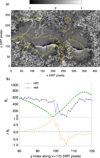 |
Fig. 6. Relative difference, δBv, on the SO/PHI-HRT image plane (see Eq. (7)). Panel a: spatial distribution of δBv. The 400 G isoline of the SO/PHI-HRT |Blos| is drawn as a solid yellow line; the purple slit at x = 170 corresponds to the location of the one-dimensional plot in panel b. Panel b, upper: profiles of the Bv components along the purple slit in panel a, for the remapped SDO/HMI (green) and SO/PHI-HRT (purple). Panel b, lower: corresponding δBv along the purple slit in panel a. |
Additional minor differences can be seen in isolated pixels of Fig. 6a (including the area around (280, 80) already noted above), and may be due to differences in calibration and RTE inversion (see the discussion in Sect. 6.1). Similarly, isolines close to unity of 1-pixel width connecting the left sunspot to the upper area are visible in the area around (100, 180). These correspond to locally vanishing values of the remapped-SDO/HMI Bv component, and should be labeled as locations of potential inaccuracy of the disambiguation in specific pixels. However, besides such smaller differences, a clear and more significant shift in the location of Bv = 0 between the two maps is incontrovertible, which shows that the assumption for a meaningful application of the SDM are violated in the double-stripe area.
To understand the consequences of the δBv double stripe on the accuracy of the SDM, we should recall the employed polar representation of the transverse component from Sect. 2.1. First, Bv is defined by Eq. (2) as a sine-function, and does not enter either Eq. (5) or Eq. (6). On the other hand, the Bw component enters both equations, and, since it is defined as a cosine function, it has large jumps at the same locations where Bv = 0, that is, at the ends of the polar angle interval of definition [0, π]. Since the difference between the Bw components estimated from each telescope enters the denominator of Eq. (5), errors in the Bw components close to location where Bv = 0 are amplified by the discontinuous character of the Bw components there, thereby heavily affecting the SDM accuracy at such locations. Indeed, the double stripe exactly corresponds to the locations of suspicious disambiguations marked by the black rectangles in Fig. 5b. A discussion of the possible origin of the double stripe is presented in Sect. 6.1.
4.3. Comparison with ME0
Next, we compared the SDM disambiguation with the standard, single-view ME0 disambiguation obtained as described in Sect. 3.1. While this is not a test for the SDM for the reason explained in Sect. 3.1, it is useful to show where differences are located that deserves further investigation.
In the comparison between the two disambiguation methods we exclude pixels where the SO/PHI-HRT transverse field is not annealed by the ME0 method, or where the transverse component is below 400 G (i.e., below the threshold set by the noise on the transverse component; see Sect. 3.1). The rate of agreement of SDM and ME0 disambiguations in this domain is 84.4%. Figure 7a render visually the spatial distribution of this agreement, where in black are represented pixels where the two methods agree, in white where they do not, and in gray pixels that are excluded from the comparison according to the criteria above.
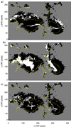 |
Fig. 7. Comparison of SDM and ME0 disambiguations on the SO/PHI-HRT image plane. The SDM is applied using information from the hmi.ME_720s_fd10 series and: Eq. (5) (panel a; see Sect. 4.1), Eq. (6) (panel b; see Sect. 4.4), and a combination of both Eqs. (5) and (6) (panel c; see Sect. 6.2). Agreement is indicated in black disagreement in white, whereas gray indicates pixels that are not considered in the comparison because the SO/PHI-HRT transverse field falls below the noise threshold; the 400 G isoline of the SO/PHI-HRT |Blos| is drawn as a solid yellow line; axes units are SO/PHI-HRT pixels. |
The SDM and ME0 disambiguations agree in most of the analyzed domain, with two exceptions: first, on the location of the double-stripe structure of Fig. 6a and, second, along the PILLoS in the northern penumbral areas. The former disagreement area is expected from the violation of the δBv = 0 necessary condition. The latter disagreement is also expected because the sign function ζ has values largely departing from the nominal ones in that area (Fig. 6a). We notice that, according to our interpretation in Sect. 4.2.1, these errors are due to fluctuations of the sign of Blos close to its PILLoS, which occur even though δBv = 0 there. Hence, both disagreements are expected from the discussion above, and they are likely true but remediable errors of the SDM (see Sects. 6 and 6.2 in particular).
4.4. Comparison of disambiguations using Eqs. (5) and (6)
In this section we consider the SDM disambiguation that is obtained by applying Eq. (6) instead of Eq. (5) to the same data and procedure as in Sect. 4.1. In this case, from the hmi.ME_720s_fd10 series, only the LoS information is used in Eq. (6). On the other hand, since the input data are the same, the co-registration and remapping procedure is identical to the one in Sect. 4.1.
The sign function ζ obtained by the application of Eq. (6) is shown in Fig. 8a, with the corresponding disambiguated magnetogram in Fig. 8b. Figure 8a shows that, in comparison with the result from Eq. (5) in Fig. 5a, there are larger areas where ζ is very different from the nominal value, ±1, with corresponding larger areas of obviously wrong disambiguation (see Fig. 8b), in particular on a relatively large patch around (x, y)≃(115, 115) and, to a smaller extent, around (x, y)≃(290, 110). The incorrect disambiguation on such areas determines a reversal of the radial component when the vector magnetogram is re-projected in heliographic coordinates (see Fig. A.1a).
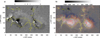 |
Fig. 8. SDM-disambiguated vector magnetograms using the hmi.ME_720s_fd10 series and Eq. (6). Panel a: sign function ζ, saturated at ±5. Panel b: vector magnetogram on the SO/PHI-HRT image plane, with Blos saturated at ±1500 G in grayscale and red and blue arrows representing the transverse field at positive and negative Blos. In both panels, the 400 G isoline of the SO/PHI-HRT |Blos| is drawn as a solid yellow line. The corresponding vector magnetogram in heliographic projection is shown in Fig. A.1a. |
The mechanism by which errors in Eq. (6) occur is analogous to Eq. (5) but involves the difference between the LoS components in the numerator of Eq. (6). Arguably, results are worse for Eq. (6) than for Eq. (5) because the angle γ is relatively small and differences between the two Blos are more affected by errors, but see also Sect. 6.1 for further discussion.
The comparison with the ME0 disambiguation is shown in Fig. 7c,d. The agreement between the two methods in this case is lower than for Eq. (5), being equal to 71%. The lower level of agreement is understood as the result of the larger areas where ζ is more strongly departing from the nominal values ±1 with respect to the case in Fig. 5a.
On the other hand, some of the penumbral areas to the north and west of the sunspots (at the location of the orange rectangles in Fig. 5b) are consistently agreeing with ME0 results, differently from what happens for Eq. (5) (cf. the two top panels in Fig. 7). Indeed, the sign obtained by Eq. (6) in these areas is homogeneously close to the nominal value, yielding a consistent disambiguation also along the PILLoS of the (SO/PHI-HRT) Blos. The reason for this improvement is that Eq. (6) involves a difference between the two Blos, which, due to the different views, have PILLoS at different locations, and is therefore less affected by fluctuations of the individual LoS components at the correspondent PILLoS. We return to this complementarity of results in Sect. 6.2.
5. SDM disambiguation using the hmi.m_45s series
In this section we use the hmi.m_45s series as input to the SDM, instead of the hmi.ME_720s_fd10 series as in Sect. 4. The hmi.m_45s data series provides the LoS magnetic field only, at a cadence of 45 s. In principle, given the shorter integration time of the hmi.m_45s data series with respect to the hmi.ME_720s_fd10 data series, the latter is more similar to the SO/PHI-HRT observation, which has 60 s integration time. This speculation is indeed confirmed by the higher correlation coefficient between the LoS components of SO/PHI-HRT and SDO/HMI found by Sinjan et al. (2023, see in particular their Table 3). The question is then if such an increased temporal homogeneity between SO/PHI-HRT and SDO/HMI inputs to the SDM is reflected in an increased accuracy of the resulting disambiguation.
On the other hand, changing to the hmi.m_45s data series has also some unavoidable consequences. First, while the availability of Blos only is not an obstacle for the application of the SDM, in such a case the co-registration procedure (step 2 in Sect. 2.3) is in principle less accurate, especially at large separation angles γ, because the different viewing angles lead to different Blos. Such an effect can indeed be a serious limitation to application of SDM when one telescope provides only LoS information and the separation angle γ is large. An accurate co-registration must be provided in other ways in such cases. Alternatively, the continuum intensity can be used instead of the magnetic field in the co-registration procedure. However, taking the comparison of Fig. 2a,b as an example, we can clearly see how the continuum intensity is also affected by both projection effects, even at relatively small separation angles, and by the difference in the resolution of the telescopes. For these reasons, we prefer to use the magnetic field for the co-registration procedure in this work, when possible. Indeed, this very topic, namely the center-to-limb variation of continuum intensity observations, is now studied using the multi-view opportunity offered by Solar Orbiter (see for instance Albert et al. 2023 and references therein).
Second, since only the LoS component is available in the hmi.m_45s series, then Eq. (6) is the only equation that can be used, given that Eq. (5) requires information about the transverse component of the field obtained from both telescopes. Therefore, insofar as the SDM equation is concerned, the case presented in this section is similar to the one discussed in Sect. 4.4, where the same Eq. (6) was applied using the LoS information from the hmi.ME_720s_fd10 data series.
The employed SDO/HMI input to the SDM procedure in Sect. 2.3 is the LoS magnetogram with the observation date March 17, 2022, 03:48:28 from the hmi.m_45s series (corresponding to T_OBS = 03:48:51 UT). The co-registration procedure using Blos associates the nominal CRVAL1,2 with CRPIX1,2 = (1232.21, 983.04), which, thanks to the relative small γ, are comparable to the co-registration shifts of Sect. 4.
Figure 9 summarizes the application of Eq. (6) to this case. Globally, the sign ζ in Fig. 9a has a very similar spatial distribution as in Fig. 8a, but shows weaker departures from the nominal ±1 values. The same is true for the disambiguated vector magnetogram (Fig. 9b) that has obvious errors in similar locations as in Fig. 8b. More in details, the areas of departures from the nominal values of the sign function ζ (in particular around (x, y)≃(115, 115) and (x, y)≃(290, 110)) appear to be slightly smaller in Fig. 9a than in Fig. 8a. Correspondingly, also the areas where a reversal of the radial component is present as a consequence of disambiguation errors are smaller, as can be seen by comparing Fig. A.1b to Fig. A.1a. Some of these differences can arguably be ascribed to the different inversion methods that the hmi.m_45s and hmi.ME_720s_fd10 data series employ (see Sect. 3.2 and also Sinjan et al. 2023, for the cross-calibration of the LoS field component between SO/PHI-HRT and the two SDO/HMI data series).
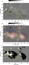 |
Fig. 9. SDM-disambiguated vector magnetogram using information from the hmi.m_45s series (see Sect. 5) on the SO/PHI-HRT image plane. Panel a: sign function ζ from Eq. (5), saturated at ±5. Panel b: vector magnetogram, with Blos saturated at ±1500 G in grayscale and red and blue arrows representing the transverse field at positive and negative Blos. Panel c: comparison of SDM and ME0 disambiguations, with agreement indicated in black, disagreement in white, and gray indicating pixels that are not considered in the comparison because the SO/PHI-HRT transverse field falls below the noise threshold. In all panels, the 400 G isoline of the SO/PHI-HRT |Blos| is drawn as a solid yellow line. The corresponding vector magnetogram in heliographic projection is shown in Fig. A.1b. |
Finally, from the point of view of the analysis of the results, since the transverse component of the SDO/HMI observation is not available in this case, then no diagnostic of the transverse component Bv is of course possible, in contrast to what is done in Sect. 4.2.2. The comparison with ME0 gives a marginally better agreement (in 73% of the selected domain) than in Sect. 4.4, with an analogous spatial distribution of the agreement/disagreement areas (cf. Fig. 9c,d with the corresponding Fig. 7c,d).
In summary, using a higher-cadence Blos magnetogram instead of a lower-cadence and longer-averaged one does improve marginally the accuracy of the SDM (ζ closer to the nominal values), but the spatial distribution of ζ is essentially the same.
6. Sources of error and future improvements
Sections 4 and 5 describe the first applications to observed data of the SDM that Paper I presented and validated using numerical simulations. Broadly speaking, the SDM produces largely spatially homogeneous and consistent disambiguations. The comparison with the ME0 method shows an agreement between SDM and ME0 that ranges from 84% (Sect. 4.3) to 71% (Sect. 4.4) of the pixels in the considered sub-domain of the FoV.
Single-viewpoint methods, such as ME0, are routinely applied (e.g., in the SDO/HMI-pipeline and in the in-development SO/PHI-pipeline), and are not restricted to the stereoscopic range of applicability as the SDM is. On the other hand, single-viewpoint methods are invariably based on assumptions, and a validation that is based on observed data only is highly desirable. We show here that the SDM, besides its direct application, may become such a reliable verification tool of single-view disambiguation methods. Our long-term goal is to attain an accuracy that allows for such verifications.
One advantage of the SDM is that it provides consistency tests to assess the quality of the obtained disambiguation in each pixel independently: first, the computed sign function ζ, which should nominally be equal to either +1 or to −1, whereas Eqs. (5) and (6) provide a continuous value that depend on observed quantities; second, the difference between the Bv components of the two telescopes, δBv, which should be zero for perfectly compatible observations. In the previous sections we positively associate anomalous values of such quantities with apparent possible errors in the SDM disambiguations. Here we discuss how such errors may arise, which tests have been made to identify their sources, and which strategies can be taken to remove them.
6.1. Possible sources of error
First of all, the SDM relies on a direct comparison of quantities observed by different instruments. The values that are compared are the product of the combined processes of spectropolarimetric data calibration and RTE inversion. Despite a relative similarity between SO/PHI-HRT and SDO/HMI, for example in terms of observed spectral line and spectral sampling (see, e.g., Solanki et al. 2020), the two telescopes have different resolutions, which affect the retrieved magnetic field (see, e.g., Stenflo 1985; Leka & Barnes 2012; Pietarila et al. 2013; DeRosa et al. 2015). Hence, a precise cross-calibration must eventually be included in the data preparation, and progress in this direction is underway (see Sinjan et al. 2023). This should also include the effect of stray light and filling factor (see, e.g., Liu et al. 2022; Leka et al. 2022), which might be different for SO/PHI-HRT and SDO/HMI. The effect of stray light is particularly important in sunspots, where it may lead to underestimations of the magnetic field strength (LaBonte 2004). In addition, the RTE inversion of the SO/PHI-HRT data set employed here (Sinjan et al. 2022) produces field maps of very high quality with a low level of noise. However, further improvements may still be possible. For instance, an RTE inversion of the SO/PHI-HRT data set using the same inversion code but different weights of the Stokes components in the fitting algorithm produced a slightly better ζ map (with a slight better agreement with ME0 of 88.7% for the case in Sect. 4) but presented some minor inversion artifacts in localized regions. On the other hand, other RTE inversions (with different parameters as well as with a different inversion code) consistently gave worse results. In other words, applications of the SDM, as of any other disambiguation method, are sensitive to the quality of RTE inversions of spectropolarimetric observations of both employed telescopes, and are expected to improve as refined inversion strategies will be developed.
Second, the SDM is based on a pixel-by-pixel comparison of observations with different resolutions and from different vantage points. This implies that the employed remapping procedure (see Sect. 2.3) must attain sub-pixel accuracy. Hence, while a co-registration of the images is not required by the SDM per se, it is unlikely that the accuracy of the pointing information of both instruments can consistently reach such a precision, and co-registration will always be necessary. The accuracy of our remapping procedure was tested using different, independently developed routines, which produced the same co-registration shifts within a fraction of a SO/PHI-HRT pixel. Figure 3 proves that residual co-registration errors are within ±2 pixels. Therefore, residual co-registration errors cannot be the origin of the double stripe in δBv that is discussed in Sect. 4 (see in particular Fig. 6b), which is on the order of 8 pixels in width. The 8-pixel shift is also larger than the amplitude of interpolation errors that could be expected by the difference in spatial resolution between SO/PHI-HRT and SDO/HMI (which is a factor of 2.6). This was verified by using different numerical schemes for the interpolation involved in the co-registration and remapping procedures. On the grounds of such tests and considerations, we tend to exclude co-registration inaccuracies as the possible origin of disambiguation errors, and of the double-stripe structure in δBv in particular.
Third, the hmi.ME_720s_fd10 series that is used as input to the SDM in Sect. 4 is the result of a relatively long average (of about 20 min, but of co-registered and properly de-rotated images) in comparison with the integration time of the SO/PHI-HRT data set (60 s), and one may wonder if that difference could ultimately generate the shift seen in δBv. However, Sect. 5 shows that similar results are obtained using the two series hmi.ME_720s_fd10 and hmi.m_45s, with the latter providing slightly better agreement with the results from applying ME0 (possibly because of the better co-temporality of the employed data sets). In a similar spirit, we applied the SDM using the hmi.ME_90s, which is a series similar to the hmi.ME_720s_fd10 series but with a cadence of 90 s instead of 720 s. Unfortunately, the hmi.ME_90s series is not readily available for all observing times, in particular not for the March 17, 2022. However, a different SO/PHI-HRT observation (March 7, 2022, described in Calchetti et al. 2023; Sinjan et al. 2023) has also a corresponding hmi.ME_90s data set, which can be used as input to the SDM. The observation date corresponds to when Solar Orbiter crossed the Earth-Sun line. While such a time is not suitable for stereoscopy (γ = 3.2°), it was still possible to study the resulting δBv, and we found a very similar double-stripe structure as for the hmi.ME_720s_fd10 series presented in this paper. Hence, from such tests, we can equally exclude that the amount of temporal averaging employed in the SDO/HMI input magnetogram plays any substantial role in the generation of the apparent misalignment of Bv components, and of the related SDM local inaccuracies. Incidentally, the presence of the double stripe also at co-alignment (and with both SO/PHI-HRT and SDO/HMI basically oriented along the solar north-south direction) also excludes that the remapping procedure plays any substantial role in generating the double stripe.
Fourth, a subtler reason for a local mismatch between observations from different viewpoints might be related to the effective depth of formation of the line seen from the two different vantage points. In short, the signal registered by two instruments pointing at the same physical location on the Sun may not come from the same parcel of plasma, due to the different optical path that the light follows in the two different directions. Such an effect is extensively discussed, and tested on numerical simulations, in Sect. 5 of Paper I. However, such an effect should decrease the more the observatories are aligned. The above-mentioned observations at Sun-Earth line crossing offered the possibility to verify the importance of this effect, and we found no significant difference in the δBv double-stripe structure. Similarly, Fig. 2 shows the presence of a horizontal light-bridge across the AR polarities, qualitatively similar to the spatial distribution of the double stripe in δBv of Fig. 6b. Due to the unmagnetized character of the plasma in the light bridge with respect to the surroundings, one could wonder if a similar optical-path effect is somehow affecting the SDM accuracy at the light-bridge location, thereby generating the double stripe in δBv. However, Fig. 10 shows that there is a clear separation between the location of the light-bridge and the δBv double stripe. Hence, the apparent misalignment is not likely to be due to such an optical-path effect.
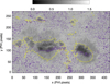 |
Fig. 10. Continuum intensity of SO/PHI-HRT (same background image as Fig. 2b) with |δBv| = 0.85 overlaid as a purple contour. The yellow solid curve represents the |Blos| = 400 G isoline. |
Fifth, the SO/PHI-HRT data that are used in this article were inverted using a standard version of the SO/PHI-HRT pipeline. In particular, as clearly visible in Fig. 2b, optical aberrations introduced by thermal effects on the entrance window and geometrical distortions are not corrected for. A procedure was recently developed to remove the former, which employs a point-spread function obtained from phase-diversity analysis, convolved with the instrument’s theoretical Airy disk. We refer the reader to Kahil et al. (2022, 2023) for more information on the phase-diversity analysis and the SO/PHI-HRT point-spread function, and to Sinjan et al. (2023), Calchetti et al. (2023) for applications that implement such a procedure. Regarding the geometrical distortion, the procedure developed to correct for it is based on a spherical distortion model retrieved from on-ground data calibration only. Concerning the SDM application considered here, some moderate increase in the noise occurs as a result of the removal of the optical aberration, which requires a fine-tuning of the ME0 disambiguation parameters for optimal performances, an effort that goes beyond the scope of this work. As a result, the SDM application is not improved by such corrections, while at the same time complicating the comparison with the ME0 method, and is not included here. However, geometrical distortions might indeed be one of the prime candidates for generating the mismatch in the Bv components associated with SDM errors, and progress in this direction is expected to significantly improve SDM results soon.
Sixth, SDO/HMI observations are affected by an uncompensated Doppler line-shift due to the spacecraft radial velocity (Hoeksema et al. 2014; Couvidat et al. 2016; Schuck et al. 2016). The employed SDO/HMI data sets are taken when the SDO radial velocity is about 2.4 km s−1, a velocity that has significant impact on the retrieved magnetic field parameters (see in particular Fig. 18 in Couvidat et al. 2016). Such an effect may impact negatively the SDM accuracy, in particular when the sign function ζ is computed using Eq. (6) as in Sects. 4.4 and 5, and even more so at relatively small γ values such as that considered here. We suspect that such an effect may contribute to the apparently worse results that are obtained in the application of Eq. (6) with respect to Eq. (5) to the particular SO/PHI-HRT data set employed here. At the time of writing, it was not possible to find SDO/HMI observations that were co-temporal with SO/PHI-HRT data and recorded at a time when the effect of the radial SDO velocity is minimal. However, new Solar Orbiter observing campaigns are planned that will provide plenty of observations at different separation angles γ, and at times when SDO/HMI radial velocity is close to zero. Such forthcoming observations will allow the ultimate effect of the SDO/HMI radial velocity on SDM accuracy to be assessed.
6.2. The best – so far – observation-based disambiguation
Finally, improvements will come from more systematic applications of the SDM itself. As already studied in Paper I, the geometrical equivalence of Eqs. (5) and (6) allows the two to be combined: in each pixel, one is free to choose for the SDM disambiguation the equation that has a higher level of reliability at that specific location. Such a decision requires practical criteria based on measurable quantities.
For instance, one can prescribe that in, each pixel, the equation that is applied is the one that yields a value of ζ that is closer to the nominal value, ±1. By applying such a criterion to the data in Sect. 4, we indeed found an improvement of the overall SDM disambiguation, with a ζ map that is, by construction, closer to the nominal values. The resulting SDM-disambiguated vector magnetogram is shown in Fig. 11a, which shows the best observation-based disambiguation obtained so far. We notice in particular that the inconsistencies around PILLoS in the penumbral areas (orange rectangles in Fig. 5b) are for the most part removed, as well as a reduced effect of the errors related to the double stripe in δBv (in the areas highlighted by the black rectangles in Fig. 5b). Similar conclusions can be drawn by comparing the disambiguated vector magnetogram in heliographic projection obtained in this case, Fig. 11b, with the correspondent magnetograms in Fig. 4b (discussed in Sect. 4.1) and Fig. A.1a,b (discussed in Sects. 4.4 and 5, respectively). Again, the combined application of Eqs. (5) and (6) yields a very significant reduction of areas of where the SDM disambiguation is suspicious, and no unexpected reversal of the radial component is present. Figure 7c shows that this combined disambiguation strategy also yields better agreement with ME0 (86.6%), especially in the eastern part of the strong field area (where Eq. (6) is selected).
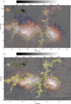 |
Fig. 11. Best – so far – observation-based SDM-disambiguated vector magnetogram. The SO/PHI-HRT vector magnetogram is disambiguated using SDO/HMI information from the (ambiguous) hmi.ME_720s_fd10 data series and a combination of Eqs. (5) and (6) (see Sect. 6.2 for details). Panel a: background image representing Blos on the SO/PHI-HRT image plane, saturated at ±1500 G in grayscale, and red and blue arrows representing the transverse field at positive and negative Blos, respectively. The 400 G isoline of |Blos| is drawn as a solid yellow line. Panel b: same as panel a but in remapped Stonyhurst coordinates, with the magnetic field re-projected in radial, poloidal, and toroidal components. In this panel, the background image represents the radial component Br saturated at ±1500 G in grayscale, and red and blue arrows represent the horizontal field at positive and negative Br, respectively. The 400 G isoline of |Br| is drawn as a solid yellow line. |
In short, the development of a quantitative criterion to combine Eqs. (5) and (6) is a promising way to further improve the accuracy and reliability of the SDM. However, before attempting a general formulation of the required decision criteria, some of the systematic errors discussed above should first be removed.
7. Conclusions
We applied the SDM to SO/PHI-HRT observations for the first time, demonstrating its viability for application to measured data beyond the proof of concept presented in Paper I. This first test employed a data set that was selected from the limited existing sample of SO/PHI-HRT observations from the first months of the science phase of Solar Orbiter. Despite the fact that the available data sets are not yet completely favorable for an optimum performance of the SDM, we provide here the first-ever observation-based, ambiguity-resolved magnetogram (Fig. 11). The intrinsic 180° ambiguity of vector magnetograms has for the first time been removed solely thanks to stereoscopic observations, without making any assumption about the properties of the photospheric magnetic field. We have proven the feasibility of the SDM approach in real applications, with very promising results overall. The best disambiguation, both in quantitative terms (i.e., the sign function ζ) and qualitative terms (smoothness and expected orientation of the transverse field component), was obtained by choosing separately in each pixel which of the two geometrically equivalent SDM formulae, Eq. (5) or Eq. (6), is closer to the nominal value, ζ = ±1.
There is nonetheless room for improvement, as localized areas of errors are also found. Such areas are associated with measurable diagnostic quantities, and we have presented several strategies for improvement.
In addition, we have presented a preliminary comparison of SDM results with a standard, single-viewpoint disambiguation method (the ME0 method from Metcalf 1994). Since standard methods are approximate insofar as they require assumptions to be made about the properties of the magnetic field, this is not a test for the SDM. However, the comparison is instructive (Fig. 7c): differences between the two disambiguations are visible at some locations close to the PILLoS of Blos in penumbral areas, which are very interesting for further studies. A very characteristic area of disagreement in the core of the sunspots is likely due to residual uncorrected geometrical distortions in SO/PHI-HRT. The currently underway improvement in the reduction of SO/PHI-HRT data is expected to greatly help reduce such artifacts.
In conclusion, the SDM fulfills the need for tools to exploit Solar Orbiter potentials for novel science, namely the stereoscopic disambiguation of vector magnetograms based on observed data only. In this way, unbiased benchmarking of single-view vector magnetograms, as well as the investigation of fundamental solar properties such as a disambiguation-independent estimation of photospheric currents that are injected in upper coronal layers, are becoming possible.
Acknowledgments
We wish to thank the referee for their competent and constructive comments that helped us improve the article. The authors thank Marco Stangalini for providing the co-registration routine, Bill Thompson for the development of the WCS routines that are part of the SolarSoft analysis package, and Pradeep Chitta for his insightful comments. E.P. acknowledges financial support from the French national space agency (CNES) through the APR program. E.P. was also supported by the French Programme National PNST of CNRS/INSU co-funded by CNES and CEA. Solar Orbiter is a space mission of international collaboration between ESA and NASA, operated by ESA. We are grateful to the ESA SOC and MOC teams for their support. The German contribution to SO/PHI is funded by the BMWi through DLR and by MPG central funds. The Spanish contribution is funded by AEI/MCIN/10.13039/501100011033/ and European Union “NextGenerationEU/PRTR” (RTI2018-096886-C5, PID2021-125325OB-C5, PCI2022-135009-2,PCI2022-135029-2) and ERDF “A way of making Europe”; “Center of Excellence Severo Ochoa” awards to IAA-CSIC (SEV-2017-0709, CEX2021-001131-S); and a Ramón y Cajal fellowship awarded to DOS. The French contribution is funded by CNES. The HMI data are courtesy of NASA/SDO and the HMI science team.
References
- Albert, K., Krivova, N. A., Hirzberger, J., et al. 2023, A&A, submitted [Google Scholar]
- Aulanier, G., Démoulin, P., Schrijver, C. J., et al. 2013, A&A, 549, A66 [NASA ADS] [CrossRef] [EDP Sciences] [Google Scholar]
- Borrero, J. M., Tomczyk, S., Kubo, M., et al. 2011, Sol. Phys., 273, 267 [Google Scholar]
- Calchetti, D., Stangalini, M., Jafarzadeh, S., et al. 2023, A&A, 674, A109 (SO Nominal Mission Phase SI) [NASA ADS] [CrossRef] [EDP Sciences] [Google Scholar]
- Couvidat, S., Rajaguru, S. P., Wachter, R., et al. 2012, Sol. Phys., 278, 217 [NASA ADS] [CrossRef] [Google Scholar]
- Couvidat, S., Schou, J., Hoeksema, J. T., et al. 2016, Sol. Phys., 291, 1887 [Google Scholar]
- DeRosa, M. L., Wheatland, M. S., Leka, K. D., et al. 2015, ApJ, 811, 107 [NASA ADS] [CrossRef] [Google Scholar]
- Forbes, T. G., Linker, J. A., Chen, J., et al. 2006, Space Sci. Rev., 123, 251 [Google Scholar]
- Freeland, S. L., & Handy, B. N. 2012, Astrophysics Source Code Library [record ascl:1208.013] [Google Scholar]
- Gandorfer, A. M., Grauf, B., Staub, J., et al. 2018, SPIE Conf. Ser., 10698, 1403 [Google Scholar]
- Gary, G. A., & Hagyard, M. J. 1990, Sol. Phys., 126, 21 [Google Scholar]
- Hoeksema, J. T., Liu, Y., Hayashi, K., et al. 2014, Sol. Phys., 289, 3483 [Google Scholar]
- Kahil, F., Gandorfer, A., Hirzberger, J., et al. 2022, SPIE Conf. Ser., 12180, 121803F [NASA ADS] [Google Scholar]
- Kahil, F., Gandorfer, A., Hirzberger, J., et al. 2023, A&A, 675, A61 (SO Nominal Mission Phase SI) [NASA ADS] [CrossRef] [EDP Sciences] [Google Scholar]
- LaBonte, B. 2004, Sol. Phys., 221, 191 [NASA ADS] [CrossRef] [Google Scholar]
- Leka, K. D., & Barnes, G. 2012, Sol. Phys., 277, 89 [NASA ADS] [CrossRef] [Google Scholar]
- Leka, K. D., Barnes, G., Crouch, A. D., et al. 2009, Sol. Phys., 260, 83 [Google Scholar]
- Leka, K. D., Wagner, E. L., Griñón-Marín, A. B., Bommier, V., & Higgins, R. E. L. 2022, Sol. Phys., 297, 121 [NASA ADS] [CrossRef] [Google Scholar]
- Li, D., & Long, D. M. 2023, ApJ, 944, 8 [NASA ADS] [CrossRef] [Google Scholar]
- Lites, B. W. 2000, Rev. Geophys., 38, 1 [Google Scholar]
- Liu, Y., Griñón-Marín, A. B., Hoeksema, J. T., Norton, A. A., & Sun, X. 2022, Sol. Phys., 297, 17 [NASA ADS] [CrossRef] [Google Scholar]
- Martínez Pillet, V. 2007, ESA Spec. Pub., 641, 27 [Google Scholar]
- Metcalf, T. R. 1994, Sol. Phys., 155, 235 [Google Scholar]
- Metcalf, T. R., Leka, K. D., Barnes, G., et al. 2006, Sol. Phys., 237, 267 [Google Scholar]
- Müller, D., St Cyr, O. C., Zouganelis, I., et al. 2020, A&A, 642, A1 [Google Scholar]
- Orozco Suárez, D., & Del Toro Iniesta, J. C. 2007, A&A, 462, 1137 [NASA ADS] [CrossRef] [EDP Sciences] [Google Scholar]
- Pesnell, W. D., Thompson, B. J., & Chamberlin, P. C. 2012, Sol. Phys., 275, 3 [Google Scholar]
- Pietarila, A., Bertello, L., Harvey, J. W., & Pevtsov, A. A. 2013, Sol. Phys., 282, 91 [NASA ADS] [CrossRef] [Google Scholar]
- Rochus, P., Auchère, F., Berghmans, D., et al. 2020, A&A, 642, A8 [NASA ADS] [CrossRef] [EDP Sciences] [Google Scholar]
- Rouillard, A. P., Pinto, R. F., Vourlidas, A., et al. 2020, A&A, 642, A2 [NASA ADS] [CrossRef] [EDP Sciences] [Google Scholar]
- Scherrer, P. H., Schou, J., Bush, R. I., et al. 2012, Sol. Phys., 275, 207 [Google Scholar]
- Schou, J., Scherrer, P. H., Bush, R. I., et al. 2012, Sol. Phys., 275, 229 [Google Scholar]
- Schuck, P. W., Antiochos, S. K., Leka, K. D., & Barnes, G. 2016, ApJ, 823, 101 [NASA ADS] [CrossRef] [Google Scholar]
- Semel, M., & Skumanich, A. 1998, A&A, 331, 383 [NASA ADS] [Google Scholar]
- Sinjan, J., Calchetti, D., Hirzberger, J., et al. 2022, SPIE Conf. Ser., 12189, 121891J [NASA ADS] [Google Scholar]
- Sinjan, J., Calchetti, D., Hirzberger, J., et al. 2023, A&A, 673, A31 (SO Nominal Mission Phase SI) [NASA ADS] [CrossRef] [EDP Sciences] [Google Scholar]
- Solanki, S. K., & Montavon, C. A. P. 1993, A&A, 275, 283 [NASA ADS] [Google Scholar]
- Solanki, S. K., del Toro Iniesta, J. C., Woch, J., et al. 2015, IAU Symp., 305, 108 [NASA ADS] [Google Scholar]
- Solanki, S. K., del Toro Iniesta, J. C., Woch, J., et al. 2020, A&A, 642, A11 [NASA ADS] [CrossRef] [EDP Sciences] [Google Scholar]
- Stenflo, J. O. 1985, Sol. Phys., 100, 189 [NASA ADS] [CrossRef] [Google Scholar]
- Sun, X. 2013, ArXiv e-prints [arXiv:1309.2392] [Google Scholar]
- Thompson, W. T. 2006, A&A, 449, 791 [NASA ADS] [CrossRef] [EDP Sciences] [Google Scholar]
- Valori, G., Löschl, P., Stansby, D., et al. 2022, Sol. Phys., 297, 12 [NASA ADS] [CrossRef] [Google Scholar]
- Volkmer, R., Bosch, J., Feger, B., et al. 2012, SPIE Conf. Ser., 8442, 84424P [NASA ADS] [Google Scholar]
- Zouganelis, I., De Groof, A., Walsh, A. P., et al. 2020, A&A, 642, A3 [NASA ADS] [CrossRef] [EDP Sciences] [Google Scholar]
Appendix A: Vector magnetograms in heliographic projection
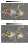 |
Fig. A.1. SDM-disambiguated vector magnetograms remapped in Stonyhurst coordinates, with the magnetic field re-projected in radial, poloidal, and toroidal components, corresponding to the cases in Fig. 8b and Fig. 9b, respectively. In both panels, the background image represents the radial component Br saturated at ±1500 G in grayscale, and red and blue arrows represent the horizontal field at positive and negative Br, respectively. The 400 G isoline of |Br| is drawn as a solid yellow line. |
All Figures
|
Fig. 1. Blos on March 17, 2022, on the image planes of SDO/HMI (left, at 03:46:35.5 UT) and SO/PHI-HRT (right, at 03:44:09 UT). The blue rectangle on the SO/PHI-HRT image shows the sub-domain that is used for co-registration (see step 2 in Sect. 2.3) and SDM application. The images are not rotated, meaning that solar north is approximately down in SDO/HMI (left) and up in SO/PHI-HRT (right). In both panels, axes are in pixels. |
| In the text | |
|
Fig. 2. Continuum images on the SO/PHI-HRT image plane of (a) remapped SDO/HMI and (b) SO/PHI-HRT data sets. The continuum intensity is normalized by its median value and shown between 0.5 and 1.2. In both panels, the isocontours of the SDO/HMI continuum intensity at [15.,25.,35.] × 103 DN s−1 (corresponding to [0.37, 0.62, 0.86] in normalized units) are drawn as solid blue lines. In panel b, the 400 G isoline of the SO/PHI-HRT |Blos| is drawn as a solid yellow line. |
| In the text | |
|
Fig. 3. Residual cross-correlation shifts after co-registration, computed in tiles of 64 × 64 pixels, in the x (panel a) and y direction (panel b). The number at the center of each tile is the co-registration shift for that tile, in units of SO/PHI-HRT pixels. Tiles where the cross-correlation procedure did not converge are marked in red. In both panels, the 400 G isoline of the SO/PHI-HRT |Blos| is drawn as a solid yellow line. |
| In the text | |
|
Fig. 4. First observation-based SDM-disambiguated vector magnetogram. The SO/PHI-HRT vector magnetogram is disambiguated using SDO/HMI information from the (ambiguous) hmi.ME_720s_fd10 data series and Eq. (5). Panel a: background image representing Blos on the SO/PHI-HRT image plane, saturated at ±1500 G in grayscale; red and blue arrows represent the transverse field at positive and negative Blos, respectively. The 400 G isoline of |Blos| is drawn as a solid yellow line. Panel b: same as panel a but in remapped Stonyhurst coordinates, with the magnetic field re-projected in radial, poloidal, and toroidal components. In this panel, the background image represents the radial component Br saturated at ±1500 G in grayscale, and red and blue arrows represent the horizontal field at positive and negative Br, respectively. The 400 G isoline of |Br| is drawn as a solid yellow line. |
| In the text | |
|
Fig. 5. Application of the SDM using the hmi.ME_720s_fd10 series and Eq. (5). Panel a: sign function ζ saturated at ±5. Panel b: corresponding SDM-disambiguated vector magnetogram, with Blos saturated at ±1500 G in grayscale and red and blue arrows representing the transverse field at positive and negative Blos (same as Fig. 4a). The rectangles in panel b indicate the areas of suspicious disambiguations discussed in Sect. 4.2 (black) and Sect. 4.2.1 (orange and green). In both panels, the 400 G isoline of the SO/PHI-HRT |Blos| is drawn as a solid yellow line. |
| In the text | |
|
Fig. 6. Relative difference, δBv, on the SO/PHI-HRT image plane (see Eq. (7)). Panel a: spatial distribution of δBv. The 400 G isoline of the SO/PHI-HRT |Blos| is drawn as a solid yellow line; the purple slit at x = 170 corresponds to the location of the one-dimensional plot in panel b. Panel b, upper: profiles of the Bv components along the purple slit in panel a, for the remapped SDO/HMI (green) and SO/PHI-HRT (purple). Panel b, lower: corresponding δBv along the purple slit in panel a. |
| In the text | |
|
Fig. 7. Comparison of SDM and ME0 disambiguations on the SO/PHI-HRT image plane. The SDM is applied using information from the hmi.ME_720s_fd10 series and: Eq. (5) (panel a; see Sect. 4.1), Eq. (6) (panel b; see Sect. 4.4), and a combination of both Eqs. (5) and (6) (panel c; see Sect. 6.2). Agreement is indicated in black disagreement in white, whereas gray indicates pixels that are not considered in the comparison because the SO/PHI-HRT transverse field falls below the noise threshold; the 400 G isoline of the SO/PHI-HRT |Blos| is drawn as a solid yellow line; axes units are SO/PHI-HRT pixels. |
| In the text | |
|
Fig. 8. SDM-disambiguated vector magnetograms using the hmi.ME_720s_fd10 series and Eq. (6). Panel a: sign function ζ, saturated at ±5. Panel b: vector magnetogram on the SO/PHI-HRT image plane, with Blos saturated at ±1500 G in grayscale and red and blue arrows representing the transverse field at positive and negative Blos. In both panels, the 400 G isoline of the SO/PHI-HRT |Blos| is drawn as a solid yellow line. The corresponding vector magnetogram in heliographic projection is shown in Fig. A.1a. |
| In the text | |
|
Fig. 9. SDM-disambiguated vector magnetogram using information from the hmi.m_45s series (see Sect. 5) on the SO/PHI-HRT image plane. Panel a: sign function ζ from Eq. (5), saturated at ±5. Panel b: vector magnetogram, with Blos saturated at ±1500 G in grayscale and red and blue arrows representing the transverse field at positive and negative Blos. Panel c: comparison of SDM and ME0 disambiguations, with agreement indicated in black, disagreement in white, and gray indicating pixels that are not considered in the comparison because the SO/PHI-HRT transverse field falls below the noise threshold. In all panels, the 400 G isoline of the SO/PHI-HRT |Blos| is drawn as a solid yellow line. The corresponding vector magnetogram in heliographic projection is shown in Fig. A.1b. |
| In the text | |
|
Fig. 10. Continuum intensity of SO/PHI-HRT (same background image as Fig. 2b) with |δBv| = 0.85 overlaid as a purple contour. The yellow solid curve represents the |Blos| = 400 G isoline. |
| In the text | |
|
Fig. 11. Best – so far – observation-based SDM-disambiguated vector magnetogram. The SO/PHI-HRT vector magnetogram is disambiguated using SDO/HMI information from the (ambiguous) hmi.ME_720s_fd10 data series and a combination of Eqs. (5) and (6) (see Sect. 6.2 for details). Panel a: background image representing Blos on the SO/PHI-HRT image plane, saturated at ±1500 G in grayscale, and red and blue arrows representing the transverse field at positive and negative Blos, respectively. The 400 G isoline of |Blos| is drawn as a solid yellow line. Panel b: same as panel a but in remapped Stonyhurst coordinates, with the magnetic field re-projected in radial, poloidal, and toroidal components. In this panel, the background image represents the radial component Br saturated at ±1500 G in grayscale, and red and blue arrows represent the horizontal field at positive and negative Br, respectively. The 400 G isoline of |Br| is drawn as a solid yellow line. |
| In the text | |
|
Fig. A.1. SDM-disambiguated vector magnetograms remapped in Stonyhurst coordinates, with the magnetic field re-projected in radial, poloidal, and toroidal components, corresponding to the cases in Fig. 8b and Fig. 9b, respectively. In both panels, the background image represents the radial component Br saturated at ±1500 G in grayscale, and red and blue arrows represent the horizontal field at positive and negative Br, respectively. The 400 G isoline of |Br| is drawn as a solid yellow line. |
| In the text | |
Current usage metrics show cumulative count of Article Views (full-text article views including HTML views, PDF and ePub downloads, according to the available data) and Abstracts Views on Vision4Press platform.
Data correspond to usage on the plateform after 2015. The current usage metrics is available 48-96 hours after online publication and is updated daily on week days.
Initial download of the metrics may take a while.