| Issue |
A&A
Volume 676, August 2023
|
|
|---|---|---|
| Article Number | A80 | |
| Number of page(s) | 27 | |
| Section | Atomic, molecular, and nuclear data | |
| DOI | https://doi.org/10.1051/0004-6361/202346436 | |
| Published online | 10 August 2023 | |
Overview of desorption parameters of volatile and complex organic molecules
A systematic dig through the experimental literature
1
Space Research & Planetary Sciences, Physics Institute, University of Bern,
3012
Bern, Switzerland
e-mail: This email address is being protected from spambots. You need JavaScript enabled to view it.
2
Aix Marseille Univ., CNRS, PIIM,
13013
Marseille, France
e-mail: This email address is being protected from spambots. You need JavaScript enabled to view it.
Received:
16
March
2023
Accepted:
8
June
2023
Abstract
Context. Many molecules observed in the interstellar medium are thought to result from the thermal desorption of ices. Parameters such as the desorption energy and pre-exponential frequency factor are essential in describing the desorption of molecules. Experimental determinations of these parameters are missing for many molecules, including those found in the interstellar medium.
Aims. The objective of this work is to expand the number of molecules for which desorption parameters are available, by collecting and re-analysing experimental temperature programmed desorption data that are present in the literature.
Methods. We used transition state theory (TST) in combination with the Redhead equation to determine the desorption parameters. Experimental data and molecular constants (e.g. mass, moment of inertia, etc.) were collected and given as input.
Results. Using the Redhead-TST method, the desorption parameters for 133 molecules were determined. The Redhead-TST method is found to provide reliable results that agree well with desorption parameters determined on the basis of more rigorous experimental methods. The importance of using accurately determined pre-exponential frequency factors to simulate desorption profiles is highlighted here. The large amount of data allows us to look for trends, with the most important being the relationship log10(v) = 2.65ln(m) + 8.07, where ν is the pre-exponential frequency factor and m is the mass of the molecule.
Conclusions. The data collected in this work allow for the thermal desorption of molecules to be modeled, with the aim of helping improve our understanding of changes in the chemical and elemental composition of interstellar environments.
Key words: astrochemistry / molecular data / methods: laboratory: solid state / methods: laboratory: molecular / solid state: volatile
© The Authors 2023
 Open Access article, published by EDP Sciences, under the terms of the Creative Commons Attribution License (https://creativecommons.org/licenses/by/4.0), which permits unrestricted use, distribution, and reproduction in any medium, provided the original work is properly cited.
This article is published in open access under the Subscribe to Open model. This email address is being protected from spambots. You need JavaScript enabled to view it. to support open access publication.
1 Introduction
The desorption of molecules from and adsorption of gaseous species on surfaces play a pivotal role in regulating physical processes and setting the chemical composition of environments in the interstellar medium (ISM), as well as regions hosting star and planet formation and Solar System objects. For example, the chemical composition of hot core and corinos, which are compact regions of warm and molecule-rich gas surrounding protostars, are largely explained by the desorption of species from ice-coated dust grains (e.g. Ligterink et al. 2018b, 2020, 2021, 2022; Bøgelund et al. 2019; Gorai et al. 2020; Yang et al. 2021; Hsu et al. 2022; Nazari et al. 2022; Bianchi et al. 2022; Zhang et al. 2023). The temperature of interstellar grains and their ice mantles dictates which molecules adsorb and consequently take part in chemical reactions (Jin & Garrod 2020; Garrod et al. 2022). The molecular composition of comets such as 67P/Churyumov-Gerasimenko is largely set by which species have remained frozen since its formation or have frozen-out on its surface since (e.g. Mumma & Charnley 2011; Goesmann et al. 2015; Altwegg et al. 2016; Rubin et al. 2019). Frozen molecules are found on the surfaces of planets and moons in the Solar System, where seasonal changes alter sublimation rates and in turn affect atmospheric processes and chemical composition (Fray & Schmitt 2009), for example, on Triton (Bertrand et al. 2022) or Pluto (Johnson et al. 2021). To interpret the observational data and model physical and chemical processes, empirical equations are employed to describe the desorption and adsorption process. For these equations, the molecule-specific parameters need to be known.
The theoretical framework and experimental methods for thermal desorption studies are well described in astrophysical and astrochemical literature (see reviews by Burke & Brown 2010; Minissale et al. 2022). In short, to simulate the desorption rate, the Polanyi-Wigner equation is generally used:
 (1)
(1)
where νn represents the pre-exponential frequency factor with value expressed in molecules1−n s−1 (also often denoted as An and where n is the desorption order with n = 0, 1, 2), N is the surface coverage in molecules cm−2 (also often denoted as θ), n (= 0, 1, 2) is the order of desorption, Edes is the desorption energy in K, and T is the temperature of the surface. The order of desorption is given as zeroth, first, or second. The zeroth order desorption is associated with multilayer desorption, while first-order desorption involves (sub)monolayer desorption. The desorption energy can also be given in Joule by changing the exponent to Edes  (kB = Boltzmann constant) or in Joule mol−1 by changing the exponent to Edes R−1 (R = ideal gas constant). Second-order desorption is possible, and is, for example, observed with processes such as recombinative desorption, where two species react to form the desorbing product. However, as this type of desorption is hardly encountered within the astrochemical literature, second-order desorption is ignored in the remainder of this publication.
There are a variety of experimental methods to determine the desorption parameters n, v, and Edes, most of them based on the temperature programmed desorption (TPD) technique or a variation thereof. In a typical TPD experiment, a surface held at low temperature under vacuum conditions is exposed and covered with a given adsorbate. Next, the temperature of the surface is linearly increased. At some point the adsorbate will start des-orbing and continues to do so until the adsorbate is fully removed from the surface. The release of adsorbate to the gas-phase can be traced with a variety of instruments, but usually a mass spectrometry technique is employed. The measured desorption trace can be analysed to find the desorption parameters, for example, via leading edge, Redhead, heating variation, inversion, or Arrhenius analysis (e.g. King 1975; De Jong & Niemantsverdriet 1990a,b; Tait et al. 2005a).
There are a number of limitations to the experimental determination of desorption parameters, specifically related to experimental efforts and safety. Currently, the number of molecules detected in the interstellar medium is about 2701,2 (McGuire 2022) and more are detected every year. Because experiments are time consuming, it is challenging to keep up with the number of detections and provide desorption parameters for all species. Furthermore, some molecules are difficult to work with, either because they are chemically unstable (e.g. PH2COOH, CH3OOH, c-C3H4O) or highly toxic (e.g. HCN, CH3NCO, H2P(O)OH). To bridge the gap between the availability of experimentally determined desorption parameters and the needs of the community, alternative approaches are needed. Computational techniques such as machine learning (Villadsen et al. 2022), Bayesian inference (Heyl et al. 2022), DFT calculations (Ferrero et al. 2022; Piacentino & Öberg 2022), or quantum mechanical methods (Germain et al. 2022; Bovolenta et al. 2022; Tinacci et al. 2022) help fill the gap. However, there also exists a rich experimental literature of TPD experiments that have been used for the identification of molecules produced in experiments that simulate chemical processes in extraterrestrial ice (known for brevity as ‘chemical TPDs’), but not to assess their desorption parameters. Because this type of data is in essence the same as what is used for the determination of desorption parameters, it raises the question of whether chemical TPD traces can be used to determine pre-exponential factors and desorption energies and, in this way, contribute more of these essential parameters to the literature.
In this study, chemical TPD traces are collected from laboratory literature and analysed with a combination of transition state theory and the Redhead method (Redhead-TST) to determine the pre-factor and desorption energies of 133 molecules. The methods are presented in Sect. 2 and the resulting data are given in Sect. 3. The implications for astrophysical and astrochemical studies are discussed in Sect. 4.
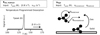 |
Fig. 1 Visual summary of the Redhead-TST method. The pre-exponential frequency factor (ν) is determined with Transition State Theory (TST). The main input are the translational ( |


2 Methods
This work makes use of an analysis method based on the Redhead equation and transition state theory, and is indicated as the Redhead-TST method throughout this manuscript. Furthermore, desorption energies and pre-exponential factors were obtained from TPD data that are used for molecule identification. The Redhead-TST method and the data set are introduced in the following sections and a visual summary is presented in Fig. 1.
2.1 Redhead-TST formalism
To determine the desorption energies of molecules from TPD data, the Redhead equation is used (Redhead 1962; King 1975):
 (2)
(2)
This equation takes the peak of the desorption trace (Tpeak, K) in combination with the heating rate (β, K s−1) and a pre-exponential factor (v, s−1) to determine Edes in K energy units. This equation only applies to first-order desorption, which generally applies to (sub)monolayer coverage. It is not used for zeroth order desorption processes, which is usually the case for multilayer desorption. Redhead (1962) showed that for v/β values of 108−1013 K−1, the relation between Edes and Tpeak is nearly linear, within a ±1.5% accuracy. For values of v/β > 1013 K−1, we verified that this relationship holds by comparing literature results with those retrieved from the Redhead equation where the same parameters are used (see Sect. 3.2). While the Redhead equation is not the most accurate analysis method for determining desorption energies (De Jong & Niemantsverdriet 1990b,a), the simplicity of this equation makes it very suitable for the analysis of TPD data that have been recorded for other purposes, such as the molecule identification, rather than their desorption parameters. Data of this type can be low in terms of the signal-to-noise ratio (SIN) or have a poorly defined desorption trace shape, which make other methods, such as the leading edge analysis (De Jong & Niemantsverdriet 199Ob,a) less suitable for their analysis.
The value for v used in the Redhead equation is usually assumed and taken to be 1012−1013 s−1. While these values are suitable for small molecules and atoms, they significantly underestimate the pre-exponential factor for larger species with more degrees of freedom. In this work, the pre-exponential factor is therefore calculated by TST, following the equation:
 (3)
(3)
where kB is the Boltzmann constant and h is the Planck constant. This formalism is adopted from Minissale et al. (2022), which is, in turn, based on work by Tait et al. (2005b). In short, TST takes the difference in rotational and translational degrees of freedom between the adsorbed and transition state into account. In Eq. (3),  and
and  are the 2D translational partition function and the 3D rotational partition function, respectively. The 2D translational partition function, because the dimension orthogonal to the surface is assumed to be common to both adsorbed and desorbed molecules.
  is given by:
 (4)
(4)
The parameter A is the surface area of each adsorbed molecule, which is fixed to 10−19 m2 and is the inverse of the generally assumed number of binding sites (that is, 1 × 1015 cm−2). For large molecules, this value could be different, but for simplicity we adopted a uniform value. Then, Λ is the thermal wavelength of the molecule and calculated as:
 (5)
(5)
In this equation, mmolecule is the mass of the particle in kg. Finally, the rotational partition function,  is given as:
 (6)
(6)
Here, σ is the symmetry factor of the molecule and indicates the number of indistinguishable orientations of the particle. Also, Ix, Iy, and Iz are the principal moments of inertia for rotation of the particle. The moments of inertia are determined using a rigid rotor approximation and chemical structures from the ChemSpider3 database. These structures are calculated with a Dreiding force field-based geometry optimisation, which is not a full quantum mechanical treatment. For a handful of molecules, their structures were not available in this database and they have been calculated with the Avogadro4 software. These equations are only applicable to molecules consisting of more than two atoms. Tait et al. (2005b) noted that this TST method gives a good approximation of the pre-exponential factor, but can overestimate the value. Adsorbates are assumed to be immobile on the surface and therefore have no rotational or translational degrees of freedom when bound (in other words qads = 1). Since some molecules are found to migrate on the surface to sites with higher binding energies, they have some degrees of freedom on the surface, which results in qads > 1. With a mobile adsorbate,  will therefore be lower, thus lowering the pre-exponential factor.
We stress that TST suffers from some limitations. One of the main approximations is that all molecules in the transition state reach the Boltzmann distribution. This could not be the case for large molecules and it is one the reasons why the TST could fail to treat large molecules. It is not easy to quantitatively define ‘large’ in this context, but based on the results of the present work and on Minissale et al. (2022), we can tentatively claim that TST starts to fail when the molecule presents more than 20 atoms. Moreover, TST neglects quantum effects, which is important at low temperatures or when the chemical reaction involves tunnelling. We point out that this a second order limitation since (except for H2 or D2 or other peculiar cases) desorption occurs at temperature where classical effects overcome of some orders of magnitude quantum effects.
Several of the species considered in this work are salt complexes, which consist of two molecules that have engaged in an acid-base reaction and are present as a cation-anion pair. For these species, it is generally not possible to determine the moments of inertia and subsequently its pre-exponential factor with TST. To determine the desorption energies of these salts, we take their pre-factor as the sum of the pre-factors of the individual acid and base. The following values are used for individual components: 4.96 × 10¹⁵ s−1 for H2O, 1.63 × 10¹⁷ s−1 for HCN, and 1.94 × 10¹⁵ s−1 for NH3 (Minissale et al. 2022) as well as 2.9 × 10¹⁷ s−1 for HNCO, 3.9 × 10¹⁷ s−1 for CH3NH2, 6.9 × 10¹⁹ s−1 for NH2COOH, 2.0 × 10¹⁸ s−1 for HCOOH, 1.3 × 10¹⁹ s−1 for CH3COOH, and 1.7 × 10²¹ s−1 for the acetaldehyde ammonia trimer (AAT, this work).
2.2 Data set
The data used in this paper have been collected from a wide variety of publications in the laboratory astrochemistry and surface science literature. All these publications make use of TPD experiments in combination with a mass spectrometry technique, such as the quadrupole mass spectrometer (QMS) or time-of-flight MS (TOF-MS) to detect and identify molecules.
To determine ERedhead and vTST, the peak desorption temperature, Tpeak, and heating rate, β, are collected and presented in Table A.2. Table A.1 lists the relevant molecular constants mass, σ, Ix, Iy, and Iz. The heating rate is usually indicated in the publication, but in cases where β is not provided, it is set to 1 K min−1. This matches with most heating rates applied in astrochemical laboratory work, but we note that heating rates in this data set range from 0.1 K min−1 to over 1 K s−1. Peak desorption temperatures can textually be indicated in the publication or be determined by eye from TPD traces presented in the figures. The absolute uncertainty on the recorded temperature is generally 0.5–2.0 K, depending on the measurement technique used (e.g. thermocouple, diode). However, a by-eye analysis of TPD data is inherently more inaccurate and the Tpeak uncertainty is therefore uniformly set to ±5 K. Combined with the uncertainties of the equations used, we applied a uniform uncertainty of ± 10% on all the determined desorption energies.
Table A.2 also list details on the substrate material, precursor molecules (i.e. starting molecule or mixture of molecules), and the ice processing source. We note that most data are collected for molecules that are formed in situ, instead of as pure or mixed deposited ices. This means that while compositions of the ice at the beginning of the experiment are given, by the time the TPD is started, this composition has changed because new molecules have been formed. In fact, some of the listed molecules may form in reactions that are promoted by heating during the TPD. This makes characterising the binding environment of a molecule challenging, as the target molecule does not only interact with the substrate or surrounding precursor species, but potentially with a host of molecules that are formed during the processing of the ice. Therefore, when the ice is processed and the target species is formed in situ, the binding environment is assumed to consist of a combination of the substrate material (e.g. metal, carbon, etc) and a residue that is a mix of different and undefined organic molecules. All molecules are assumed to be present at (sub)monolayer coverage (1 ML ≈ 1 × 10¹⁵ molecules cm−2), unless there is clear mention that multilayer quantities (≫1 ML) of product are formed, for example, those determined from IR spectroscopic measurements, in which case the molecule is excluded from the dataset.
It is possible that the molecule under investigation is co-desorbed with another matrix species, namely, either a precursor molecule or a new species that is abundantly formed during the processing of the ice. Because co-desorbing species have a peak desorption temperature that is governed by the matrix molecule instead of the binding of the targeted species to the surface, these molecules are excluded from the data set. For precursor molecules (e.g. H2O, CH3OH) desorption temperatures are often known and therefore any target molecule that has a Tpeak close to this is considered to be co-desorbing and excluded. However, during processing new molecules that act as co-desorption matrix can be formed. Because the full molecular inventory is not always described, it is difficult to identify co-desorption in these cases. It is only if there is mention or a strong suspicion that co-desorption is occuring that the entry would be omitted.
A variety of ice processing techniques are used, ranging from UV and X-ray processing to hydrogenation and electron or ion bombardment. We note that thermal processing is also a possibility, but this is only listed when it is explicitly mentioned as a step in the molecule formation process. The TPD process itself is not considered as thermal processing.
Finally, data on (sub)monolayer desorption studies presented in the literature have also been collected and presented in Table A.2 as well. In some cases, only vlit and Elit are presented, while in other cases sufficient information is available (i.e. Tpeak and β) that vTST and ERedhead can also be determined.
3 Results and discussion
In Table A.2, data on 133 molecules from 132 publications have been collected, for a total of 328 entries. Information on the CHNOPS elemental composition, functional groups, and binding surfaces in the data set are presented in Fig. 2. The vast majority of molecules contain one or more carbon and hydrogen atoms, while a substantial fraction contain at least one oxygen atom. About one-third of the molecules included contain at least one nitrogen atom, while phosphorus and sulfur are present in a minor percentage of the data set. In terms of functional groups, we find that mostly alchols, aldehydes or ketones, and amines are covered in the data set. Contrary to what is found in the ISM (e.g. Cernicharo et al. 2020, 2022; McGuire et al. 2020; Marcelino et al. 2021; Lee et al. 2021b,a, 2022; Loomis et al. 2021), cyanides only make up a small portion of this data set and ethers and formates represent the smallest fraction of the functional groups.
This figure highlights the large availability of experimental data on oxygen-bearing molecules, but relatively few molecules are covered that contain nitrogen, phosphorus, or sulfur atoms. There are two primary explanations for this. First, many precursor molecules with N, P, or S, such as HCN, PH3, and H2S, are more difficult to work with in the laboratory or toxic – therefore experimental researchers tend to avoid them. In turn, a lesser amount of TPD data on the formation of molecules containing these kinds of atoms is available. At the same time the limited amount of data available on N, P, and S-bearing species may also indicate that ice chemistry is less efficient at forming such molecules or that molecules containing these atoms are refractory and do not desorb at temperature ≤300 K.
Finally, the cold surfaces for these studies are dominated by metallic ones (e.g. Au, Ag, Pt). Surfaces that are more relevant to the ISM, such as crystalline or amorphous water, highly oriented pyrolytic graphite (HOPG), graphene, silica (SiO2), and silicates ( ) make up a smaller percentage of the data set. Only a few ice chemistry experiments have made use of surfaces that are not metallic (e.g. Potapov et al. 2022). Since many molecules in the data set are obtained from such experiments, this explains the dominance of metallic surfaces in the data set. However, as mentioned earlier in this paper, these molecules are produced in situ, likely together with a mixture of other complex organic molecules that can remain on the surface at temperatures ≥300 K. Consequently, the binding surface of the target molecule will be a combination of the metallic surface and an organic molecular residue. This environment be a relevant analogue to dust grains in the ISM, which are presumably coated in a layer of organic molecules once water-ice is removed from their surfaces. In the following sections, a deeper look will be taken at the Redhead-TST method performance and collected desorption energy and pre-exponential factor data.
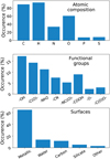 |
Fig. 2 Occurrences of CHNOPS atoms (top panel), functional groups (middle panel), and binding surfaces (bottom panel) of the entries present in the data set used in this paper. The category labelled ‘other’ in the bottom panel includes surfaces such as KBr and MgF2 windows. |
3.1 Influence of TPD data on the Redhead-TST output
The Redhead-TST method relies on TPD data, which can show major differences in Tpeak between experiments. Consequently, this influences the derived vTST and Eredhead−TST values. Examples of this are shown in Fig. 3, where vTST and Eredhead−TST of all entries of CH3CH2CHO (propionaldehyde), CH3COCOCH3 (2,3-butanedione), NH2OH (hydroxylamine), (CH2OH)2 (ethyleneglycol), HOCHCHOH (1,2-ethenediol), HOCH2CH(OH)CHO (glyceraldehyde), and HOCH(CH2OH)2 (glycerol) are shown. In all cases, marginal variations of at most one order of magnitude are seen in the pre-exponential factors for each molecule. Variations on this level will have a negligible effect on the simulated desorption profiles. However, in several cases, large shifts in the retrieved desorption energy are found, with the most extreme scatter seen in CH3COCOCH3 values, which range from 6920 to 12 690 K. These shifts are directly correlated with the peak desorption temperature used as input for the Redhead equation.
The scatter in peak desorption temperatures and, thus, desorption energies, can be explained through several scenarios. First and foremost, the coverage of a species of interest is not known in the majority of cases; therefore, molecules can span a wide range of (sub)monolayer coverages. At a lower coverage, molecules have a tendency to settle in deeper binding sites, which have higher desorption energies. Consequently, there is a correlation between coverage and desorption temperature, where lower coverage results in a shift of desorption to higher temperature (see e.g. Smith et al. 2016; He et al. 2016). This effect is more pronounced on rough surfaces, which have a broad range of binding sites, such as amorphous solid water (ASW) or the organic residue that is presumably formed in the experiments included in this work.
The surface on which the experiment is conducted can also play a role. Almost all entries depicted in Fig. 3 are measured on a metallic surface, but this classification groups many different materials, such as Au, Ag, and Cu, as well as structures such as rough Pt(111) or Mo(110) together. Each metal and surface structure will result in different desorption energies, which in turn shift the value of Tpeak. This shift is exacerbated when other categories of surfaces are used, such as water ice or carbon. For the selected molecules, a clear example is seen for NH2OH. One entry is measured on graphite (Ioppolo et al. 2014) and its retrieved desorption energy is a clear outlier with respect to the other entries of this molecule. Similarly, the type of organic residue formed on a surface during an experiment can also influence the desorption characteristics. This is highlighted by CH3COCOCH3, for which all entries are measured on the same type of Ag surface, but produced with different irradiated precursors, such as CH3CHO, CH3CHO:CH3COCOCH3, and H2O:CH3CHO.
Since the desorption parameters of molecules covered in this study have (in most cases) not been reported, the values listed in this work can be used as an approximation of the pre-factor and desorption energy, for example, in chemical models. However, it is important to be aware that the provided values are limited by the quality of the TPD input data.
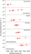 |
Fig. 3 Values of vTST and Eredhead−TST of all the entries of H3CH2CHO (propionaldehyde), CH3COCOCH3 (2,3-butanedione), NH2 OH (hydroxylamine), (CH2OH)2 (ethyleneglycol), HOCHCHOH (1,2-ethenediol), HOCH2CH(OH)CHO (glyceraldehyde), and HOCH(CH2OH)2 (glycerol). Symbols indicate a metallic surface (squares) or carbon surface (pentagon, NH2OH panel). |
3.2 Redhead-TST method performance
In Fig. 4, the Redhead-TST and literature Edes and v values are compared for a number of publications where both these values are available. The top panel of this figure shows the pre-factors values, which are colored based on whether the difference Δ(νΤSΤ − vLit) is smaller than +3 orders of magnitude (red squares) or larger than +3 orders of magnitude (blue circles). The literature v values that are in close agreement with their TST counterpart are found to derive from studies that employ more rigorous methods to determine the pre-factor (e.g. Tait et al. 2005b; Chaabouni et al. 2018; Behmard et al. 2019; Tylinski et al. 2020), although a number of data points are also derived from studies that in fact employ the same TST to calculate v (Ulbricht et al. 2006). To some extent, the large differences in pre-factors are not surprising, as in many studies v is assumed to be 1012 or 1013 s−1. This tendency is visible in the top panel of Fig. 4. We conclude that the TST method gives accurate approximations of the pre-exponential factor value.
The subsequent effect of the adopted v on the desorption energy is visible in the bottom panel of Fig. 4. The data points in the bottom panel are again labeled according to the difference in pre-factor values. When the difference in v is ≤3 decades, the desorption energies are in good agreement and fall on the parity line. Contrary, when there is a large difference between vlit and vTST there is a prominent difference between ERedhead and Elit. Because in all these cases, the literature pre-factor is lower than vTST, the corresponding desorption energy is also lower. This comparison shows that the Redhead-TST method gives accurate desorption parameters that are in good agreement with those derived in experiments, provided these experimental parameters are determined with rigorous laboratory and analysis methods.
We could argue that the large discrepancies between ERedhead−TST and Elit when vlit is assumed will not actually affect the simulated desorption behaviour, as in either case the best-fit parameters are generated. An example of this is shown in Fig. 5, where the data of the molecules CH3NCO (methyl isocyanate), CH3C(0)NH2 (acetamide), and NH2C(O)NH2 (carbamide) are analysed with the Redhead-TST method (red lines) and the Redhead method, while assuming v = 1013 s−1. The dashed lines show the simulated desorption profiles at a heating rate of 5 K min−1, the same temperature ramp as used in the studies where the TPD data of these molecules are taken from (Ligterink et al. 2017, 2018a). The peak desorption temperatures determined with a TST and assumed prefactor are found to be identical and match with the Tpeak value determined in the laboratory. However, if the heating rate is changed to 1 K century−1, a value that is applicable to interstellar environments, the peak desorption temperatures show a substantial deviation. The simulated profiles with the assumed v value, which are lower than the value determined with TST, underestimate the peak desorption temperature by about 10%. This example highlights the importance of determining desorption parameters, including the pre-exponential factor, as accurately as possible. However, it is important to be aware of the nuances of heating in interstellar environments. Grains can be heated by photons and in the case of very small particles and energetic photons, the grains can be flash heated at rates on the order of K s−1. In these cases, desorption energies with assumed pre-exponential factors might be just as applicable, as shown by Fig. 5. In general, it is recommended that as accurate a value as possible be used.
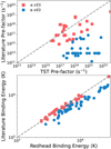 |
Fig. 4 Comparison between v (top panel) and Edes (bottom panel) values obtained from literature sources, but which have also been analysed with the Redhead-TST method. Red squares indicate entries for which the difference between vTST and vlit is smaller than three orders of magnitude, whereas the blue circles indicate those with a difference larger than three orders of magnitude. |
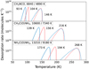 |
Fig. 5 Desorption traces of CH3NCO, CH3C(0)NH2, and NH2C(O)NH2 with desorption parameters obtained with the Redhead-TST method (red) and the Redhead method, assuming a pre-exponential factor of 1013 s−1 (blue). Peak desorption temperatures are indicated in the plot for each species. The desorption profile is simulated with a first-order Polanyi-Wigner equation, surface coverage of 1×10¹⁵ molecules cm2, and heating rate of 1 K century−1 (solid lines), which is appropriate for the ISM, or the heating rate of 5 K min−1 (dashed lines) used in these experiments. |
3.3 Data trends
Due to the large amount of collected data, it is possible to investigate trends in pre-factor values and desorption energies. In Fig. 6, Edes (top panels) and v (bottom panels) are plotted against the molecule mass in amu (left column) and number of atoms of the molecule (right column). Data points obtained with the Redhead-TST method are indicated in red, while those taken from literature are presented in blue. In addition, the recommended desorption parameters of molecules from various surfaces listed in Minissale et al. (2022) have been added in green points (data from their Tables 2 and 3). Each data point is labelled by its surface castegory, which includes metallic (squares), carbon (pentagons), silicate (triangles), and water-ice (circles).
Both Redhead-TST and literature desorption energies show a general tendency to increase with increasing molecule mass or number of atoms. However, most striking is the large spread in desorption energy values for a given molecular mass or number of atoms, which often spans more than 5000 K (top panels Fig. 6). This spread makes it difficult to retrieve any empirical relationship between the parameters. Even when only data of a specific surface or containing certain functional groups are selected (not shown), no trend or relationship is found.
The situation is different for the pre-exponential factors. While the laboratory literature data is affected by the tendency to assume v = 1013 s−1, there is a clear trend in the TST data showing a relationship between vTST and the molecule mass. These data are fitted with an equation of the form log10(v) = a·ln(m) + b, where m is the mass of the molecule in amu (atomic mass units, and the best-fit values are found to be a = 2.65 and of b = 8.07. Because both studied make use of TST to determine the pre-factor, the data points of both this work (red) and those of Minissale et al. (2022; green) are used for the fit. The TST data points show a scatter of about one decade around the best-fit line, an uncertainty that has a marginal effect on any simulated desorption profile. The recommended values presented by Minissale et al. (2022) are in good agreement with the found equation and show that the equation can also be used for lower mass molecules. This empirical relationship can be used to estimate the pre-exponential factor of a molecule solely based on its mass. This may find use when analysing laboratory data to determine Edes values or as an easy way to determine pre-factors for molecules in astrochemical models (see also Sect. 4.1).
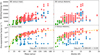 |
Fig. 6 Desorption energy (top row) and pre-exponential factor (bottom row) plotted against molecule mass (left column) and number of atoms (right column). Values derived with the Redhead-TST method are coloured in red, recommended desorption parameters adopted from Minissale et al. (2022) in green, and other literature sources are presented in blue. Marker symbol indicates whether a molecule is desorbing from a metallic (squares), water (circles), silicate (triangle), or carbon (pentagon) surface. |
3.4 Desorption parameters and caveats
For several molecules, a large number of entries of the same species have been collected in Table A.2. This amount of data can be useful in several cases, such as to analyse the influence of the desorption surface. However, often a single v and Edes value is desired, for example, to be used chemical models. The mean values for v and Edes for molecules analysed in this work with the Redhead-TST method are presented Table 1.
It is important to note several caveats of the data provided in Table 1. First, these desorption parameters are the mean of the available data. Monolayer desorption is a more nuanced process and desorption energies will differ depending on coverage and available binding sites. The mean values presented in this table should only be used when no data is available from more rigorous studies and only for specific applications, such as input for astrochemical models.
Second, binding environments are grouped together, but one has to be aware that the desorption energies of these molecules will be different when, for example, amorphous water ice or graphite are considered. The most prominent source of desorption parameter data comes from experiments that make use of metallic surfaces (e.g. Au, Ag, and Pt substrates). Often the molecule is formed in situ together with other species, and there the binding surface can be seen as a combination of metallic and a refractory organic residue, which makes these environments more realistic.
In connection to the above points, it is important to note that for some molecules extensive studies have been performed to determine the pure ice (sub)monolayer desorption parameters, including on different surfaces. In particular molecules that are often and abundantly observed in the ISM are on this list, such as CH3NH2, CH3CHO, HCOOH, CH3CH2OH, CH3OCHO, CH3COOH, and HOCH2CHO (e.g. Lattelais et al. 2011; Bertin et al. 2011; Burke et al. 20l5a,b,c; Chaabouni et al. 2018; Corazzi et al. 2021; Ferrero et al. 2022). While these studies are invaluable to assess the influence of different binding environments, in many cases the pre-exponential frequency factor is assumed (e.g. to be 1012 or 1013 s−1), which will affect the determined desorption energy. In Table A.2 the Redhead-TST analysis of these data are presented when possible. If desorption parameters on surfaces like amorphous or crystalline water, HOPG, or silicates are required, it is recommended to adopt these values.
While some molecules are well studied, it is also noteworthy that some prominent interstellar molecules have not rigorously been studied in the laboratory, such as dimethyl ether (CH3OCH3), ethylene glycol ((CH2OH)2), and acetamide (CH3C(O)NH2). For some molecules like ethyl-cyanide (CH3CH2CN) and vinylcyanide (CH2CHCN), only limited data can be found in the literature (Toumi et al. 2016; Kimber et al. 2018; Couturier-Tamburelli et al. 2018) and only for the case of multilayer desorption. Because these species are routinely observed in the ISM (e.g. Nazari et al. 2022), dedicated laboratory studies of these molecules are desired. The parameters of these molecules presented in this study rely solely on chemical TPD data and should be considered the best currently available.
Mean desorption parameters.
4 Astrophysical implications
4.1 Impact of the pre-factor on astrochemical models
Astrochemical models make use of the Polanyi-Wigner equation or a variation thereof to calculate the desorption rates of molecules on dust grains (e.g. Kulterer et al. 2020). While for these models desorption energies are generally taken from experimental and theoretical literature, the v value is calculated with an empirical formula, often the harmonic oscillator relation presented in Hasegawa et al. (1992):
 (7)
(7)
which uses the molecule mass, m, the molecule binding energy, Edes, and the number of binding sites per grain surface area, nss, as input to calculate the pre-factor. Except for small molecules and atoms, this equation underestimates the value of v, often by multiple decades (Minissale et al. 2022). This is also found for molecules considered in this study. Figure 7 shows the difference between vTST and VHasegawa and visualises the fact that for the majority of cases, vTST is at least seven decades larger than the pre-factor calculated with the Hasegawa equation.
The difference in the adopted pre-factor can have a strong impact on astrochemical models. Combining a desorption energy that is determined with Redhead-TST or any other accurate method with a pre-factor determined by the Hasagawa equation can severely misrepresent the desorption behaviour of the molecule (see Fig. 2 in Ceccarelli et al. 2022). This is exemplified in Fig. 8 for the molecules CH3NCO, CH3C(O)NH2, and NH2C(O)NH2. For these species, ERedhead−tst is determined with data from Ligterink et al. (2017, 2018a) and subsequently plotted with vTST (red) and vHasegawa (blue). The desorption profiles (left panel) plotted with vHasegawa are all shifted to higher temperatures and misrepresent the actual desorption profile. For these examples, the peak desorption temperature is about 30% higher than what it should be. In the right panel, the gas and ice column densities are plotted against the radius of a protoplanetary disk, which has the average temperature profile T(r) = 200 × (r/1 AU)0.62 K, as found by Andrews & Williams (2007). For each 1 K temperature step, the number of desorbed molecules is determined, and when summed, this gives the gas-phase column density; when subtracted from a starting value of 1 × 1015 cm−2, it gives the ice column density. As expected from their peak desorption temperatures, the ice-gas inversion point lies at a larger radius when the accurate TST pre-factor is used. Using vHasegawa results in the inversion point shifting ~50% inwards.
Due to its impact on astrochemical models, it is recommended to use more accurate pre-exponential factor values. One way is to implement the empirical equation presented in Sect. 3.3, with the caveat that this equation is ill suited to determine pre-factors for atoms and diatomic molecules. Better yet, it is all the more handy to use the v and Edes that belong together as presented in the literature source as direct input for the chemical model, to prevent any misrepresentation.
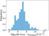 |
Fig. 7 Difference between VTST and vHasagawa for molecules presented in this study. Frequencies normalised to one are presented. |
4.2 Peak desorption temperatures
For simplicity and consistency, desorption profiles and peak desorption temperatures are calculated using Eq. (1) and a heating rate of 1 K century−1 in this work. However, this heating rate is not appropriate for all interstellar environments and peak desorption temperatures are often determined with other equations, such as the adsorption-thermal-desorption balance presented by Hasegawa et al. (1992; see also Nazari et al. 2021):
 (8)
(8)
As input, this equation takes the grain size agrain (set to 0.1 µm), the grain number density, ngrain (set to 1.0 × 10⁻¹² nH, with nH the gas density), the sticking efficiency, S (set to 1), the gas and grain temperature, T, the molecule mass, m, the molecule binding energy, Edes, and the number of binding sites per grain surface area, nss, to calculate the ice-to-gas ratio. The peak desorption temperature is taken as the point where ice and gas molecular abundances are equal, that is, nice/ngas = 1. Instead of the peak desorption temperature depending on the heating rate values, in this equation it primarily depends on the gas density of the environment. Furthermore, we note that this equation in its original form makes use of the harmonic oscillator relation to calculate the pre-exponential frequency in the denominator. As discussed in Sect. 4.1, this equation gives inaccurate values for larger molecules and therefore the equation should rather take accurate pre-factor into account:
 (9)
(9)
Using the latter equation, the peak desorption temperatures where calculated for nH = 1 × 107 cm−3 (appropriate for molecular clouds) and nH = 1 × 1012 cm−3 (appropriate for protoplanetary disk environments) and compared with the Tpeak determined from the peak of the Polanyi-Wigner desorption profile using a heating rate of β = 1 K century−1. Desorption parameters listed in Table 1 were used. In Table 2 the results for a selection of twenty molecules are presented.
The adsorption-thermal-desorption equation a low density (nH = 1 × 107 cm−3) shows a small difference with the Polanyi-Wigner results. One aspect that affects this comparison is the definition of the peak desorption temperature of the adsorption-thermal-desorption balance equation, which is located at the point where nice / ngas = 1. However, for the Tpeak from the Polanyi-Wigner equation this is usually nice / ngas ≤ 0.1. Correcting for this discrepancy raises the adsorption-thermal-desorption balance peak desorption temperatures by several K. In turn, this make Tpeak,PW and Tpeak,ATD for the low-density scenario virtually identical. Quite different is the situation for the high-density (nH = 1 × 1012 cm−3) results of the adsorption-thermal-desorption balance equation, which show peak desorption temperatures that are approximately 20% higher than those obtained with the Polanyi-Wigner equation. The peak desorption temperatures listed in this study might therefore not be representative for all interstellar environments and source-specific modelling is required to accurately determine desorption fronts.
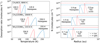 |
Fig. 8 Comparison of desorption profiles generated with the TST (red) or the Hasegawa (blue) prefactor. Left panel: Desorption profiles of CH3NCO, CH3C(O)NH2, and NH2C(O)NH2. The desorption energies are determined with the Redhead-TST method using data from Ligterink et al. (2017, 2018a; see Table A.2 and top left corners). Desorption profiles are plotted for vTST (red) and with vHasegawa (blue). The desorption profile is simulated with a first-order Polanyi-Wigner equation, surface coverage of 1 × 10¹⁵ molecules cm−2, and heating rate of 1 K century−1. Peak desorption temperatures decrease by ~30% when realistic pre-factors are used. Right panel: Ice (solid) and gas (dashed) abundances plotted against radius (au) of a protoplanetary disk for vTST (red) and with vHasegawa (blue). An average disk temperature profile of T(r) = 200 × (r/1 AU)0.62 K is used (Andrews & Williams 2007). For each 1 K temperature step, the number of desorbed molecules is determined, which summed give the gas-phase column density and subtracted from a starting value of 1 × 1015 cm−2 give the ice column density. The TST abundances are offset by a factor of 10 for easier viewing. The peak radii of the ice-gas inversion are indicated and are shown to shift outward by ~50% when realistic pre-factors are used. |
Comparison peak desorption temperatures.
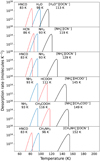 |
Fig. 9 Desorption profiles of acids (red), bases (blue), and the resulting salt (black). Desorption energies and pre-factors for H2O, NH3, and HCN are obtained from Minissale et al. (2022), while the parameters for the remaining molecules are taken from Table 1. Peak desorption temperatures are indicated in the plot for each species. The desorption profile is simulated with a first-order Polanyi-Wigner equation, surface coverage of 1015 molecules cm−2 and heating rate of 1 K century−1. |
4.3 Salt desorption
Several molecules detected in the interstellar medium can be classified as acids ([AH], e.g. HCOOH, HNCO, CH3COOH) or bases ([B], e.g. NH3, CH3NH2). In ice mantles, these species can engage in acid-base reactions and form organic salts via the reaction [AH] + [B] → [A−][BH+]. Several such salts are included in this study and their desorption energies are determined. The pre-factors of these salts are determined by adding the pre-exponential factor values of its individual components ([AH] and [B]), see Sect. 2.1. While there is a chemical diversity in the salts, they often include ammonia as the base. In the interstellar medium, ammonia is also expected to be a prominent base, due to its high ice abundance (up to 10% w.r.t. H2O, Boogert et al. 2015). In all cases, Edes of the salt is larger than the value of its individual components and therefore the salts will reside on dust grains at higher temperatures (see also e.g. Kruczkiewicz et al. 2021). This is exemplified in Fig. 9 where the desorption profiles of various salts and their corresponding acid and base are plotted. A first-order Polanyi-Wigner equation is used, with a monolayer coverage of 1015 molecules cm−2 and a heating rate of 1 K century−1. Differences in peak desorp-tion temperatures range from just over 10 K for the H2O-HNCO system, to more than 60 K for the CH3NH2-HNCO system.
The ability to lock up molecules in the form of salts can carry a number of implications. Large quantities of organic molecules with amino (-NH2) or carboxylic acid (-COOH) groups can be trapped in organic salt complexes and remain on dust grains and larger bodies at elevated temperatures. Recent analysis of samples collected and return from the astroid Ryugu show that it contains high concentrations of amines (e.g. CH3NH2) and acids (HCOOH and CH3COOH, Naraoka et al. 2023). Because these molecules are found to not be trapped in minerals or other organic matter, the authors suggest that these species reside in the material as salts in order to explain why these volatiles are still present. Our results underline this conclusion, although questions remains if the salts included in this study, which are still relatively volatile, could have survived the heating (≥300 K) and hydrothermal stages during the formation of Ryugu (Nakamura et al. 2022). Further desorption studies of salts complexes could help unravel in which salt form amines and acids are locked up in asteroid Ryugu.
Organic salt complexes also provide a molecular reservoir that remains available for grain surface chemistry for a longer time (or rather to higher temperatures), but not for gas-phase reactions. Ammonia is the dominant nitrogen carrier in observed interstellar ice, but it is also relatively volatile. Locking ammonia up in ammonium salts ( ) could mean that a substantial atomic nitrogen reservoir is available on interstellar grains long after NH3 or H2O have desorbed (see Fig. 9). Laboratory investigations of the processing of salts with energetic radiation at elevated temperatures (≥100 K) and in water-free environments are relevant avenues for investigating the formation of prebiotic molecules (see for example Bossa et al. 2009b).
As salts desorb at higher temperatures, they can give misleading indications of sublimation fronts as determined with observations of interstellar environments. For example, Lee et al. (2022) measured the spatial distribution of various molecules toward the HH212 protoplanetary disk and found similar radial distributions of HNCO and NH2CHO. If the presence of these molecules in the gas can entirely be explained by ice desorption, this co-spatial distribution is peculiar as these molecules have significantly different desorption parameters of 2.9 × 10¹⁷ s −1 and 5154 K (this work) and 3.69 × 10¹⁸ s−1 and 9561 K (Minissale et al. 2022) for HNCO and NH2CHO, respectively. We would expect that HNCO desorbs at a much lower temperature or larger radius than NH2CHO. However, if instead most of the HNCO available in the ice has reacted with NH3, it would be locked up in the [NH+][OCN−] salt. This salt has the desorption parameters 2.9 × 10¹⁷ s−1 and 8117 K, which are close to those of formamide. The salt can therefore explain the co-spatial distribution of HNCO and NH2CHO due to thermal desorption of the [NH+][OCN−] salts, which, upon desorption, dissociates into its individual components, HNCO and NH3 (see also Lee et al. 2022).
Thus far, two molecules have been detected in the interstellar medium that are presumed to be part of salt complexes. These are the cyanate anion (OCN−) and the ammonium cation  (Lacy et al. 1984; Keane et al. 2001; Pontoppidan et al. 2003; Van Broekhuizen et al. 2005). Recently, these species have also been detected in observations with the new James Webb Space Telescope (JWST, McClure et al. 2023). The unprecedented sensitivity of JWST opens up two avenues of research. Firstly, it is possible to look for other salt components at lower abundance or with weaker spectroscopic features, for example, the cyanide anion (CN−) and carboxylate anions (R-COO−). Secondly, searches for salts in water poor or free interstellar environments, for example, molecular clouds that interact with the warm gas of a protostellar outflow or the edges of photo-dominated regions (PDRs), can be conducted. Because the bulk ice species have been removed from the grains in these regions, the less abundant salt and organic species are easier to detect. Furthermore, the presence and shape of salt spectroscopic signatures will provide information about the chemical and physical history of the environment.
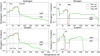 |
Fig. 10 Ice elemental composition as [X]/[carbon] for hydrogen, nitrogen, oxygen, and sulphur as a function of temperature. Peak desorption temperatures for selected species are indicated in the plot (vertical dashed lines). Elemental compositions of soluble organic matter (SOM) obtained from the Murchison meteorite (Schmitt-Kopplin et al. 2010) and averaged insoluble organic matter (IOM, Alexander et al. 2017) are indicated (horizontal dashed lines). The desorption profiles are simulated with a first-order Polanyi-Wigner equation, variable surface coverages, and a heating rate of 1 K century−1. Low and high OM values represent low and high fraction of organic molecules, respectively. |
4.4 Chemical and elemental composition above the water-snow line
Within star- and planet-forming environments, temperature gradients and the associated desorption fronts of molecules, also called snow lines, play an important role in forming planetary objects and setting their chemical and elemental composition. Examples of such lines are the nitrogen and water snowline or the soot line, which is driven by the sublimation of large carbon-dominated molecules such as polycyclic aromatic hydrocarbons (PAHs). These lines are invoked to explain the high atomic nitrogen abundance in Jupiter or the comparatively low carbon content of Earth (Bosman et al. 2019; Öberg & Bergin 2021; Li et al. 2021). Because of their high abundances, observational, modelling, and experimental efforts have focused on the main ice species to investigate desorption fronts. Since most organic molecules except for CH3OH and CH4 are found at low abundances, these species will not affect the elemental composition of a protoplanetary disk or create snow lines that are observable. However, the combined inventory of organic molecules may affect the elemental composition. ISO and Spitzer IR observation of various interstellar sources have found significant features in the 5–8 µm region (Gibb & Whittet 2002; Boogert et al. 2008). These features have at least in part been assigned to an organic residue consisting of a variety of molecules, including HCOOH and HCOO−. Therefore, the data presented in this paper are used in this section to investigate how a large reservoir of diverse organic molecules affects elemental ratios and the chemical composition, for example in a protoplanetary disk.
Elemental ratios of hydrogen, nitrogen, oxygen, phosphorus, and sulphur over carbon are determined for a molecular inventory that consists of the species listed in this work and desorption parameters presented in Table 1, supplemented by bulk ice species with parameters taken from Table 3 of Minissale et al. (2022). The ice abundances are set with respect to water. The following fractions are used: CO, N2, and CO2 at 0.25, CH3OH at 0.1, O2, CH4, NH3, and H2CO at 0.05, and H2S, CS, and HCN at 0.01. Combined, the aforementioned species are indicated as the bulk ice species. All remaining organic molecules listed in this work, as well as C2H2, CH3CN, and NH2CHO taken from Minissale et al. (2022) are included in a low and high fraction scenario where each organic molecule contributes at 10−4 and 10−3 level, respectively. The desorption profile, including ice and gas abundances are simulated with a first-order Polanyi-Wigner equation, variable abundances according to fractions with respect to water, and a heating rate of 1 K century−1. The elemental composition is obtained by multiplying the ice or gas abundance of each molecule with its elemental composition (e.g. for CH3OH carbon = abundance × 1, hydrogen = abundance × 4, and oxygen = abundance × 1) and subsequently summing all contributions to an element.
The resulting ice elemental compositions for [hydrogen]/[carbon], [nitrogen]/[carbon], [oxygen]/[carbon], and [sulphur]/[carbon] are shown in Fig. 10. Figure B.1 shows the same plot, but with elemental ratios plotted versus protoplanetary disk radius by using an average protoplanetary disk temperature profile T(r) = 200 × (r/1 AU)0.62 K (Andrews & Williams 2007). The elemental ratio of [phosphorus]/[carbon] is shown in Fig. B.2. The bulk ice elemental ratios are plotted in blue, while the addition of a low (10−4×[H2O]) and high (l·0−3×[H2O]) fraction of organic molecules are plotted in red and green, respectively. The peak desorption temperatures of several bulk ice species are indicated, as well as the elemental composition of the extraterrestrial substances soluble organic matter (SOM, Sephton 2002) and insoluble organic matter (IOM, Alexander et al. 2017). Both SOM and IOM are regularly extracted from meteorites and SOM shows similarities with the organic material measured on several Solar System objects, such as comet 67P/ Churyumov-Gerasimenko (Hänni et al. 2022). In this work, we use the average elemental composition of C100H155N3O20S3 for SOM obtained from the Murchison meteorite (Schmitt-Kopplin et al. 2010) and the average IOM composition of C100H77O14N3S2 presented in Alexander et al. (2017).
Firstly, we note that the addition of organic material affects the elemental ratios at low temperatures, when bulk ice dominates. The combined contribution of organic elemental carbon lowers all elemental ratios. The effect is most pronounced for the high fraction organic matter model where it can lower ratios by up to 100%. In this scenario, we only take the contribution of the 133 molecules studied in this work into account. In a natural environment the diversity of the organic components may be many times larger (e.g. Hänni et al. 2022) and therefore have an even larger impact on elemental ratios.
Secondly, we note the importance of the organic material to set the ice elemental composition when the bulk ice species are removed from the solid state. In our model, all the bulk ice species are lost before ~ 115 K, while the species that contribute to the nitrogen and sulphur budget are gone at lower temperatures of ~ 100 and ~75 K, respectively. These differences in bulk ice desorption explain the dips seen in [N]/[C] and [S]/[C] between 75 and 100 K. At these points the nitrogen (NH3) and sulphur (CS) reservoirs have desorbed, but the main carrier of carbon (CH3OH) is still present. It is likely that these dips will be less pronounced in reality due to the trapping of the volatile nitrogen and sulphur carriers in the dominating water-phase, which desorbs together methanol. After desorption of the bulk ice reservoir the organic material starts to dominate the overall elemental composition on the dust grains.
The elemental ratios are biased towards the molecules included in this work and the assumption that molecules contribute equally to the total molecular budget is unlikely to be realistic. Therefore, care needs to be taken with any interpretation of Fig. 10. However, some general observations can be made. First, at low temperature(≤115 K) or larger radii (≥3 au), the bulk ices dominate the elemental budget and ratios are seen to vary in a stepwise manner. Objects formed in this regime will have predictable elemental compositions, depending on the “step” they form at. However, in the warmer disk regions closer to the (proto)star and where water has desorbed, the elemental budget is set by the large mixture of organic molecules, which desorb at different temperatures. Consequently, the elemental composition is seen to be much more varied, especially in [hydrogen]/[carbon] and [oxygen]/[carbon]. Objects that form in this regime could thus be expected to have a much more varied or less predictable elemental signature.
It is interesting to point out that the organic molecules that remain on the grains at T ≥ 100 K show similarities with and, in some cases, are identical to, the molecules used by Kudo et al. (2002) to determine the sticking velocity of organics-coated grains. These authors found that organics-coated grains rapidly coagulate in the 2.3–3.0 au region of a disk. This region is in good agreement with the location where we find most organic molecules still coating the grains after water has desorbed.
Finally, the evolution of various functional chemical groups are plotted in Fig. 11. The abundances of the functional groups have been determined in the same way that the elemental abundances have. Ratios of amides ([-NC(O)-]), cyanides ([-CN]), alcohols ([-OH]), carboxylic acids ([-COOH]), aldehydes + ketones ([-C(O)-]), esters ([-C(O)O-]), and ethers ([-O-]) with respect to amines ([-NH2]) are plotted. This plot reflects several observations already made in Sect. 3 about the occurrence in of certain functional groups in the data set, for example that the alcohol (-OH) group is most abundant. It also shows that some of these functional groups can be quickly depleted as the environment warms up. In particular esters and ethers will be removed quickly. On the other hand, amides and amines seem to remain present to higher temperatures. In this way we see how chemical make-up and average properties of an organics-coated grain may change with temperature and could potentially be used as a tracers of thermal history of a particle in the Solar System. However, it is important to acknowledge that this view is biased towards relatively small and volatile organic molecules. For example, IOM is rich in ether (-O-) cross links (Remusat et al. 2005) and because this substance is very refractory it will ensure that the ether functional group will remain prominent component of the organic coating of grains at elevated temperatures.
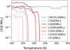 |
Fig. 11 Functional chemical group composition [X]/[-NH2] for oxygen-bearing groups -OH, -COOH, -C(O)-, -C(O)O-, and -O- (solid red lines) and nitrogen-bearing groups -NC(O)- and -CN (dashed blue lines) as a function of temperature. The desorption profiles are simulated with a first-order Polanyi-Wigner equation, variable surface coverages, and a heating rate of 1 K century−1. |
5 Conclusion
This study presents a large number of desorption parameters, namely, desorption energies (Edes) and pre-exponential frequency factors (v). These parameters will find use in astrochemical models and help to understand the evolution of the chemical and elemental composition in star- and planet-forming regions. Because the list of molecules is dominated by organic molecules and salts of medium-volatility these data are of particular importance to assess the surface chemistry in regions were water ice has been removed from dust grains.
To expand the number of molecules for which desorption parameters are available, experimental temperature programmed desorption data have been collected from the literature and analysed with the Redhead-transition state theory (Redhead-TST) method to determine the pre-exponential frequency factor (v) and the desorption energy (E). A comparison with literature v and Edes values shows that the Redhead-TST method provides reliable results that are on par with results of rigorous experimental methods. We emphasise that the usage of accurately determined pre-factor values, instead of assumed values or the often used Hasagawa equation, is essential to properly simulate the desorption profiles of molecules. Due to the large amount of data collected in this study, trends can be searched for. No relationship between molecule mass or number of atoms is found, but a relationship between the pre-factor and molecule mass in the form of log10(v) = 2.65ln(m) + 8.07 is, which can be used to determine this parameter in future studies. Mean des-orption parameters are provided and used to highlight how the desorption of these species can affect chemical and elemental compositions.
Avogadro: an open-source molecular builder and visualisation tool. Version 1.2.0 http://avogadro.cc/
Appendix A Desorption parameters and molecular constants
The analysis techniques used in this publication make use of a number of molecular constants, such as the moments of inertia, molecule mass, and symmetry factor, which are listed in Table A.1. All the literature studies used in this work and the pre-exponential frequency factors and desorption energies determined with the Redhead-TST method are presented in Table A.2. This table provides an overview of all relevant data to determine the desorption constants (that is, Tpeak, β), but also information on the desorption surface and how the molecule was produced.
Molecular constants
Literature and Redhead-TST desorption energies
Appendix B Elemental ratios
Based on the desorption parameters found in this work and assumed abundances, the ice elemental composition is determined throughout a protoplanetary disk, see Sect. 4.4. The radial variations in elemental ratios are presented in Fig. B.1. Figure B.2 presents the [Phosphorus]/[Carbon] ratio plotted against temperature.
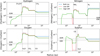 |
Fig. B.1 Ice elemental composition as [X]/[Carbon] for Hydrogen, Nitrogen, Oxygen, and Sulphur as a function of protoplanetary disk radius. Peak desorption radii for selected species are indicated in the plot (vertical dashed lines). Elemental compositions of Soluble Organic Matter (SOM) obtained from the Murchison meteorite (Schmitt-Kopplin et al. 2010) and averaged Insoluble Organic Matter (IOM) (Alexander et al. 2017) are indicated (horizontal dashed lines). The desorption profiles are simulated with a first-order Polanyi-Wigner equation, variable surface coverages, and a heating rate of 1 K century−1. An average protoplanetary disk temperature profile of T(r) = 200 × (r/1AU)0.62 (Andrews & Williams 2007) is used to determine the radii. |
 |
Fig. B.2 Ice elemental composition [Phosphorus]/[Carbon] as a function of temperature. The desorption profiles are simulated with a first-order Polanyi-Wigner equation, variable surface coverages, and a heating rate of 1 K century−1. |
Acknowledgements
The authors thank E. F. van Dishoeck, E. G. Bøgelund, and C. Ceccarelli for helpful discussions and feedback. Thanks go out to K.-J. Chuang for making unpublished TPD plots of CH2CHNH2 and CH3CHNH available for analysis. The authors thank the many astrochemists and surface scientists who have contributed data to the literature on which this study relies. N.F.W.L. acknowledges support from the Swiss National Science Foundation (SNSF) Ambizione grant 193453 and NCCR PlanetS. M.M. acknowledges the French national programme “Physique et Chimie du Milieu Interstellaire” (PCMI) of CNRSIINSU with INCIINP cofunded by CEA and CNES.
References
- Abplanalp, M. J., & Kaiser, R. I. 2019, PCCP, 21, 16949 [NASA ADS] [CrossRef] [Google Scholar]
- Abplanalp, M. J., Borsuk, A., Jones, B. M., & Kaiser, R. I. 2015, ApJ, 814, 45 [Google Scholar]
- Abplanalp, M. J., Förstel, M., & Kaiser, R. I. 2016, Chem. Phys. Lett., 644, 79 [NASA ADS] [CrossRef] [Google Scholar]
- Abplanalp, M. J., Frigge, R., & Kaiser, R. I. 2019, Sci. Adv., 5, eaaw5841 [NASA ADS] [CrossRef] [Google Scholar]
- Alexander, C. O., Cody, G., De Gregorio, B., Nittler, L., & Stroud, R. 2017, Geochemistry, 77, 227 [NASA ADS] [CrossRef] [Google Scholar]
- Altwegg, K., Balsiger, H., Bar-Nun, A., et al. 2016, Sci. Adv., 2, e1600285 [NASA ADS] [CrossRef] [Google Scholar]
- Andrews, S. M., & Williams, J. P. 2007, ApJ, 659, 705 [NASA ADS] [CrossRef] [Google Scholar]
- Bahr, S., & Kempter, V. 2007, J. Chem. Phys., 127, 074707 [CrossRef] [Google Scholar]
- Behmard, A., Fayolle, E. C., Graninger, D. M., et al. 2019, ApJ, 875, 73 [Google Scholar]
- Bergantini, A., Abplanalp, M. J., Pokhilko, P., et al. 2018a, ApJ, 860, 108 [NASA ADS] [CrossRef] [Google Scholar]
- Bergantini, A., Frigge, R., & Kaiser, R. I. 2018b, ApJ, 859, 59 [NASA ADS] [CrossRef] [Google Scholar]
- Bergantini, A., Góbi, S., Abplanalp, M. J., & Kaiser, R. I. 2018c, ApJ, 852, 70 [NASA ADS] [CrossRef] [Google Scholar]
- Bergantini, A., Zhu, C., & Kaiser, R. I. 2018d, ApJ, 862, 140 [NASA ADS] [CrossRef] [Google Scholar]
- Bergner, J. B., Öberg, K. I., Rajappan, M., & Fayolle, E. C. 2016, ApJ, 829, 85 [NASA ADS] [CrossRef] [Google Scholar]
- Bertin, M., Romanzin, C., Michaut, X., Jeseck, P., & Fillion, J.-H. 2011, J. Phys. Chem. C, 115, 12920 [NASA ADS] [CrossRef] [Google Scholar]
- Bertin, M., Doronin, M., Fillion, J.-H., et al. 2017, A&A, 598, A18 [NASA ADS] [CrossRef] [EDP Sciences] [Google Scholar]
- Bertrand, T., Lellouch, E., Holler, B., et al. 2022, Icarus, 373, 114764 [NASA ADS] [CrossRef] [Google Scholar]
- Bianchi, E., López-Sepulcre, A., Ceccarelli, C., et al. 2022, ApJ, 928, L3 [NASA ADS] [CrossRef] [Google Scholar]
- Bisschop, S., Fuchs, G., Boogert, A., Van Dishoeck, E., & Linnartz, H. 2007, A&A, 470, 749 [NASA ADS] [CrossRef] [EDP Sciences] [Google Scholar]
- Boamah, M. D., Sullivan, K. K., Shulenberger, K. E., et al. 2014, Faraday Discuss., 168, 249 [NASA ADS] [CrossRef] [Google Scholar]
- Bøgelund, E. G., Barr, A. G., Taquet, V., et al. 2019, A&A, 628, A2 [NASA ADS] [CrossRef] [EDP Sciences] [Google Scholar]
- Boogert, A. C., Pontoppidan, K. M., Knez, C., et al. 2008, ApJ, 678, 985 [NASA ADS] [CrossRef] [Google Scholar]
- Boogert, A. A., Gerakines, P. A., & Whittet, D. C. 2015, ARA&A, 53, 541 [NASA ADS] [CrossRef] [Google Scholar]
- Bosman, A. D., Cridland, A. J., & Miguel, Y. 2019, A&A, 632, L11 [NASA ADS] [CrossRef] [EDP Sciences] [Google Scholar]
- Bossa, J., Theule, P., Duvernay, F., & Chiavassa, T. 2009a, ApJ, 707, 1524 [Google Scholar]
- Bossa, J.-B., Duvernay, F., Theulé, P., et al. 2009b, A&A, 506, 601 [NASA ADS] [CrossRef] [EDP Sciences] [Google Scholar]
- Bossa, J.-B., Borget, F., Duvernay, F., et al. 2012, Aust. J. Chem., 65, 129 [CrossRef] [Google Scholar]
- Bovolenta, G. M., Vogt-Geisse, S., Bovino, S., & Grassi, T. 2022, ApJS, 262, 17 [NASA ADS] [CrossRef] [Google Scholar]
- Burke, D. J., & Brown, W. A. 2010, PCCP, 12, 5947 [NASA ADS] [CrossRef] [Google Scholar]
- Burke, D., Wolff, A., Edridge, J., & Brown, W. 2008, J. Chem. Phys., 128, 104702 [NASA ADS] [CrossRef] [Google Scholar]
- Burke, D. J., Puletti, F., Brown, W. A., et al. 2015a, MNRAS, 447, 1444 [CrossRef] [Google Scholar]
- Burke, D. J., Puletti, F., Woods, P. M., et al. 2015b, J. Phys. Chem. A, 119, 6837 [NASA ADS] [CrossRef] [Google Scholar]
- Burke, D. J., Puletti, F., Woods, P. M., et al. 2015c, J. Chem. Phys., 143, 164704 [NASA ADS] [CrossRef] [Google Scholar]
- Butscher, T., Duvernay, F., Danger, G., & Chiavassa, T. 2016, A&A, 593, A60 [NASA ADS] [CrossRef] [EDP Sciences] [Google Scholar]
- Carrascosa, H., Cruz-Díaz, G., Muñoz Caro, G. M., Dartois, E., & Chen, Y. 2020, MNRAS, 493, 821 [CrossRef] [Google Scholar]
- Ceccarelli, C., Codella, C., Balucani, N., et al. 2022, arXiv e-prints [arXiv:2206.13270] [Google Scholar]
- Cernicharo, J., Marcelino, N., Agúndez, M., et al. 2020, A&A, 642, L8 [NASA ADS] [CrossRef] [EDP Sciences] [Google Scholar]
- Cernicharo, J., Fuentetaja, R., Cabezas, C., et al. 2022, A&A, 663, L5 [NASA ADS] [CrossRef] [EDP Sciences] [Google Scholar]
- Chaabouni, H., Diana, S., Nguyen, T., & Dulieu, F. 2018, A&A, 612, A47 [NASA ADS] [CrossRef] [EDP Sciences] [Google Scholar]
- Chaabouni, H., Baouche, S., Diana, S., & Minissale, M. 2020, A&A, 636, A4 [Google Scholar]
- Chuang, K.-J., Fedoseev, G., Qasim, D., et al. 2020, A&A, 635, A199 [EDP Sciences] [Google Scholar]
- Congiu, E., Fedoseev, G., Ioppolo, S., et al. 2012, ApJ, 750, L12 [NASA ADS] [CrossRef] [Google Scholar]
- Corazzi, M. A., Brucato, J. R., Poggiali, G., et al. 2021, ApJ, 913, 128 [NASA ADS] [CrossRef] [Google Scholar]
- Coupeaud, A., Piétri, N., Allouche, A., Aycard, J.-P., & Couturier-Tamburelli, I. 2008, J. Phys. Chem. A, 112, 8024 [NASA ADS] [CrossRef] [Google Scholar]
- Couturier-Tamburelli, I., Toumi, A., Piétri, N., & Chiavassa, T. 2018, Icarus, 300, 477 [NASA ADS] [CrossRef] [Google Scholar]
- Danger, G., Borget, F., Chomat, M., et al. 2011a, A&A, 535, A47 [NASA ADS] [CrossRef] [EDP Sciences] [Google Scholar]
- Danger, G., Bossa, J.-B., De Marcellus, P., et al. 2011b, A&A, 525, A30 [NASA ADS] [CrossRef] [EDP Sciences] [Google Scholar]
- Danger, G., Duvernay, F., Theulé, P., Borget, F., & Chiavassa, T. 2012, ApJ, 756, 11 [Google Scholar]
- Danger, G., Rimola, A., Abou Mrad, N., et al. 2014, PCCP, 16, 3360 [NASA ADS] [CrossRef] [Google Scholar]
- De Jong, A., & Niemantsverdriet, J. 1990a, Vacuum, 41, 232 [NASA ADS] [CrossRef] [Google Scholar]
- De Jong, A., & Niemantsverdriet, J. 1990b, Surf. Sci., 233, 355 [CrossRef] [Google Scholar]
- Demers, L. M., Östblom, M., Zhang, H., et al. 2002, J. Am. Chem. Soc., 124, 11248 [CrossRef] [Google Scholar]
- DeSimone, A. J., Olanrewaju, B. O., Grieves, G. A., & Orlando, T. M. 2013, J. Chem. Phys., 138, 084703 [NASA ADS] [CrossRef] [Google Scholar]
- Dostert, K.-H., O’Brien, C. P., Mirabella, F., Ivars-Barceló, F., & Schauermann, S. 2016, PCCP, 18, 13960 [NASA ADS] [CrossRef] [Google Scholar]
- Duvernay, F., Dufauret, V., Danger, G., et al. 2010, A&A, 523, A79 [NASA ADS] [CrossRef] [EDP Sciences] [Google Scholar]
- Duvernay, F., Danger, G., Theulé, P., Chiavassa, T., & Rimola, A. 2014, ApJ, 791, 75 [NASA ADS] [CrossRef] [Google Scholar]
- Eckhardt, A. K., Bergantini, A., Singh, S. K., Schreiner, P. R., & Kaiser, R. I. 2019, Angew. Chem., 131, 5719 [NASA ADS] [CrossRef] [Google Scholar]
- Fedoseev, G., Cuppen, H. M., Ioppolo, S., Lamberts, T., & Linnartz, H. 2015a, MNRAS, 448, 1288 [NASA ADS] [CrossRef] [Google Scholar]
- Fedoseev, G., Ioppolo, S., Zhao, D., Lamberts, T., & Linnartz, H. 2015b, MNRAS, 446, 439 [NASA ADS] [CrossRef] [Google Scholar]
- Fedoseev, G., Chuang, K.-J., van Dishoeck, E. F., Ioppolo, S., & Linnartz, H. 2016, MNRAS, 460, 4297 [NASA ADS] [CrossRef] [Google Scholar]
- Fedoseev, G., Chuang, K.-J., Ioppolo, S., et al. 2017, ApJ, 842, 52 [NASA ADS] [CrossRef] [Google Scholar]
- Ferrero, S., Grieco, F., Ibrahim Mohamed, A., et al. 2022, MNRAS, 516, 2586 [CrossRef] [Google Scholar]
- Förstel, M., Maksyutenko, P., Jones, B., et al. 2016a, Chem. Commun., 52, 741 [CrossRef] [Google Scholar]
- Förstel, M., Tsegaw, Y. A., Maksyutenko, P., et al. 2016b, Chem. Phys. Chem., 17, 2726 [CrossRef] [Google Scholar]
- Förstel, M., Bergantini, A., Maksyutenko, P., Góbi, S., & Kaiser, R. I. 2017, ApJ, 845, 83 [Google Scholar]
- Fray, N., & Schmitt, B. 2009, Planet. Space Sci., 57, 2053 [Google Scholar]
- Frigge, R., Zhu, C., Turner, A. M., et al. 2018a, ApJ, 862, 84 [NASA ADS] [CrossRef] [Google Scholar]
- Frigge, R., Zhu, C., Turner, A. M., et al. 2018b, Chem. Commun., 54, 10152 [CrossRef] [Google Scholar]
- Garrod, R. T., Jin, M., Matis, K. A., et al. 2022, ApJS, 259, 1 [NASA ADS] [CrossRef] [Google Scholar]
- Germain, A., Tinacci, L., Pantaleone, S., Ceccarelli, C., & Ugliengo, P. 2022, ACS Earth Space Chem., 6, 1286 [Google Scholar]
- Gibb, E., & Whittet, D. 2002, ApJ, 566, L113 [NASA ADS] [CrossRef] [Google Scholar]
- Goesmann, F., Rosenbauer, H., Bredehöft, J. H., et al. 2015, Science, 349, aab0689 [Google Scholar]
- Gorai, P., Bhat, B., Sil, M., et al. 2020, ApJ, 895, 86 [Google Scholar]
- Guennoun, Z., Couturier-Tamburelli, I., Piétri, N., & Aycard, J.-P. 2005, J. Phys. Chem. B, 109, 3437 [CrossRef] [Google Scholar]
- Hänni, N., Altwegg, K., Combi, M., et al. 2022, Nat. Commun., 13, 1 [Google Scholar]
- Hasegawa, T. I., Herbst, E., & Leung, C. M. 1992, ApJS, 82, 167 [Google Scholar]
- He, J., Vidali, G., Lemaire, J.-L., & Garrod, R. T. 2015, ApJ, 799, 49 [NASA ADS] [CrossRef] [Google Scholar]
- He, J., Acharyya, K., & Vidali, G. 2016, ApJ, 825, 89 [Google Scholar]
- Heyl, J., Holdship, J., & Viti, S. 2022, ApJ, 931, 26 [NASA ADS] [CrossRef] [Google Scholar]
- Hsu, S.-Y., Liu, S.-Y., Liu, T., et al. 2022, ApJ, 927, 218 [NASA ADS] [CrossRef] [Google Scholar]
- Ioppolo, S., Van Boheemen, Y., Cuppen, H., Van Dishoeck, E., & Linnartz, H. 2011, MNRAS, 413, 2281 [NASA ADS] [CrossRef] [Google Scholar]
- Ioppolo, S., Fedoseev, G., Minissale, M., et al. 2014, PCCP, 16, 8270 [NASA ADS] [CrossRef] [Google Scholar]
- Ioppolo, S., Fedoseev, G., Chuang, K.-J., et al. 2021, Nat. Astron., 5, 197 [NASA ADS] [CrossRef] [Google Scholar]
- Jimenez-Escobar, A., & Muñoz Caro, G. 2011, Mol. Universe, 280, 153 [NASA ADS] [Google Scholar]
- Jin, M., & Garrod, R. T. 2020, ApJS, 249, 26 [Google Scholar]
- Johnson, P. E., Young, L. A., Protopapa, S., et al. 2021, Icarus, 356, 114070 [NASA ADS] [CrossRef] [Google Scholar]
- Jones, B. M., Kaiser, R. I., & Strazzulla, G. 2014, ApJ, 788, 170 [NASA ADS] [CrossRef] [Google Scholar]
- Kaiser, R. I., & Maksyutenko, P. 2015, Chem. Phys. Lett., 631, 59 [CrossRef] [Google Scholar]
- Keane, J., Tielens, A., Boogert, A., Schutte, W., & Whittet, D. 2001, A&A, 376, 254 [NASA ADS] [CrossRef] [EDP Sciences] [Google Scholar]
- Kimber, H. J., Toscano, J., & Price, S. D. 2018, MNRAS, 476, 5332 [NASA ADS] [CrossRef] [Google Scholar]
- King, D. A. 1975, Surf. Sci., 47, 384 [NASA ADS] [CrossRef] [Google Scholar]
- Kleimeier, N. F., & Kaiser, R. I. 2021, J. Phys. Chem. Lett., 13, 229 [Google Scholar]
- Kleimeier, N. F., Eckhardt, A. K., Schreiner, P. R., & Kaiser, R. I. 2020a, Chem, 6, 3385 [CrossRef] [Google Scholar]
- Kleimeier, N. F., Turner, A. M., Fortenberry, R. C., & Kaiser, R. I. 2020b, Chem. Phys. Chem., 21, 1531 [CrossRef] [Google Scholar]
- Kleimeier, N. F., Abplanalp, M. J., Johnson, R. N., et al. 2021a, ApJ, 911, 24 [NASA ADS] [CrossRef] [Google Scholar]
- Kleimeier, N. F., Eckhardt, A. K., & Kaiser, R. I. 2021b, J. Am. Chem. Soc., 143, 14009 [CrossRef] [Google Scholar]
- Kruczkiewicz, F., Vitorino, J., Congiu, E., Theulé, P., & Dulieu, F. 2021, A&A, 652, A29 [NASA ADS] [CrossRef] [EDP Sciences] [Google Scholar]
- Kudo, T., Kouchi, A., Arakawa, M., & Nakano, H. 2002, Meteor. Planet. Sci., 37, 1975 [NASA ADS] [CrossRef] [Google Scholar]
- Kulterer, B. M., Drozdovskaya, M. N., Coutens, A., Manigand, S., & Stéphan, G. 2020, MNRAS, 498, 276 [Google Scholar]
- Lacy, J., Baas, F., Allamandola, L., et al. 1984, ApJ, 276, 533 [NASA ADS] [CrossRef] [Google Scholar]
- Lasne, J., Laffon, C., & Parent, P. 2012, PCCP, 14, 697 [NASA ADS] [CrossRef] [Google Scholar]
- Lattelais, M., Bertin, M., Mokrane, H., et al. 2011, A&A, 532, A12 [NASA ADS] [CrossRef] [EDP Sciences] [Google Scholar]
- Layssac, Y., Gutiérrez-Quintanilla, A., Chiavassa, T., & Duvernay, F. 2020, MNRAS, 496, 5292 [NASA ADS] [CrossRef] [Google Scholar]
- Lee, K. L. K., Changala, P. B., Loomis, R. A., et al. 2021a, ApJ, 910, L2 [NASA ADS] [CrossRef] [Google Scholar]
- Lee, K. L. K., Loomis, R. A., Burkhardt, A. M., et al. 2021b, ApJ, 908, L11 [CrossRef] [Google Scholar]
- Lee, C.-F., Codella, C., Ceccarelli, C., & López-Sepulcre, A. 2022, ApJ, 937, 10 [NASA ADS] [CrossRef] [Google Scholar]
- Leroux, K., Guillemin, J.-C., & Krim, L. 2021, MNRAS, 507, 2632 [CrossRef] [Google Scholar]
- Li, J., Bergin, E. A., Blake, G. A., Ciesla, F. J., & Hirschmann, M. M. 2021, Sci. Adv., 7, eabd3632 [NASA ADS] [CrossRef] [Google Scholar]
- Ligterink, N., Coutens, A., Kofman, V., et al. 2017, MNRAS, 469, 2219 [Google Scholar]
- Ligterink, N., Terwisscha van Scheltinga, J., Taquet, V., et al. 2018a, MNRAS, 480, 3628 [NASA ADS] [CrossRef] [Google Scholar]
- Ligterink, N. F. W., Calcutt, H., Coutens, A., et al. 2018b, A&A, 619, A28 [NASA ADS] [CrossRef] [EDP Sciences] [Google Scholar]
- Ligterink, N. F., El-Abd, S. J., Brogan, C. L., et al. 2020, ApJ, 901, 37 [Google Scholar]
- Ligterink, N., Ahmadi, A., Coutens, A., et al. 2021, A&A, 647, A87 [NASA ADS] [CrossRef] [EDP Sciences] [Google Scholar]
- Ligterink, N. F., Ahmadi, A., Luitel, B., et al. 2022, ACS Earth Space Chem., 6, 455 [NASA ADS] [CrossRef] [Google Scholar]
- Liu, G., Rodriguez, J., Chang, Z., Hrbek, J., & González, L. 2002, J. Phys. Chem. B, 106, 9883 [NASA ADS] [CrossRef] [Google Scholar]
- Loomis, R. A., Burkhardt, A. M., Shingledecker, C. N., et al. 2021, Nat. Astron., 5, 188 [NASA ADS] [CrossRef] [Google Scholar]
- Mahjoub, A., Poston, M. J., Blacksberg, J., et al. 2017, ApJ, 846, 148 [NASA ADS] [CrossRef] [Google Scholar]
- Maity, S., Kaiser, R. I., & Jones, B. M. 2014, Faraday Discuss., 168, 485 [NASA ADS] [CrossRef] [Google Scholar]
- Maity, S., Kaiser, R. I., & Jones, B. M. 2015, PCCP, 17, 3081 [NASA ADS] [CrossRef] [Google Scholar]
- Maksyutenko, P., Martín-Doménech, R., Piacentino, E. L., Öberg, K. I., & Rajappan, M. 2022, ApJ, 940, 113 [NASA ADS] [CrossRef] [Google Scholar]
- Marcelino, N., Tercero, B., Agúndez, M., & Cernicharo, J. 2021, A&A, 646, L9 [NASA ADS] [CrossRef] [EDP Sciences] [Google Scholar]
- Marks, J. H., Wang, J., Evseev, M. M., et al. 2023, ApJ, 942, 43 [NASA ADS] [CrossRef] [Google Scholar]
- McClure, M. K., Rocha, W., Pontoppidan, K., et al. 2023, Nat. Astron., 7, 1 [Google Scholar]
- McGuire, B. A. 2022, ApJS, 259, 30 [NASA ADS] [CrossRef] [Google Scholar]
- McGuire, B. A., Burkhardt, A. M., Loomis, R. A., et al. 2020, ApJ, 900, L10 [Google Scholar]
- McManus, J. R., Martono, E., & Vohs, J. M. 2014, Catal. Today, 237, 157 [CrossRef] [Google Scholar]
- Minissale, M., & Dulieu, F. 2014, J. Chem. Phys., 141, 014304 [NASA ADS] [CrossRef] [Google Scholar]
- Minissale, M., Aikawa, Y., Bergin, E., et al. 2022, ACS Earth Space Chem., 6, 597 [NASA ADS] [CrossRef] [Google Scholar]
- Muir, M., Molina, D. L., Islam, A., Abdel-Rahman, M. K., & Trenary, M. 2020, PCCP, 22, 25011 [NASA ADS] [CrossRef] [Google Scholar]
- Mumma, M. J., & Charnley, S. B. 2011, ARA&A, 49, 471 [NASA ADS] [CrossRef] [Google Scholar]
- Nakamura, T., Matsumoto, M., Amano, K., et al. 2022, Science, 379, eabn8671 [Google Scholar]
- Naraoka, H., Takano, Y., Dworkin, J. P., et al. 2023, Science, 379, eabn9033 [CrossRef] [Google Scholar]
- Nazari, P., van Gelder, M., Van Dishoeck, E., et al. 2021, A&A, 650, A150 [NASA ADS] [CrossRef] [EDP Sciences] [Google Scholar]
- Nazari, P., Meijerhof, J., van Gelder, M., et al. 2022, A&A, 668, A109 [NASA ADS] [CrossRef] [EDP Sciences] [Google Scholar]
- Noble, J., Theule, P., Duvernay, F., et al. 2014, PCCP, 16, 23604 [NASA ADS] [CrossRef] [Google Scholar]
- Noble, J., Diana, S., & Dulieu, F. 2015, MNRAS, 454, 2636 [NASA ADS] [CrossRef] [Google Scholar]
- Oba, Y., Watanabe, N., Kouchi, A., Hama, T., & Pirronello, V. 2010, ApJ, 722, 1598 [CrossRef] [Google Scholar]
- Öberg, K. I., & Bergin, E. A. 2021, Phys. Rep., 893, 1 [Google Scholar]
- Östblom, M., Liedberg, B., Demers, L. M., & Mirkin, C. A. 2005, J. Phys. Chem. B, 109, 15150 [CrossRef] [Google Scholar]
- Peck, J. W., Mahon, D. I., & Koel, B. E. 1998, Surf. Sci., 410, 200 [NASA ADS] [CrossRef] [Google Scholar]
- Piacentino, E. L., & Öberg, K. I. 2022, ApJ, 939, 93 [NASA ADS] [CrossRef] [Google Scholar]
- Pontoppidan, K., Fraser, H., Dartois, E., et al. 2003, A&A, 408, 981 [NASA ADS] [CrossRef] [EDP Sciences] [Google Scholar]
- Potapov, A., Theulé, P., Jäger, C., & Henning, T. 2019, ApJ, 878, L20 [NASA ADS] [CrossRef] [Google Scholar]
- Potapov, A., Fulvio, D., Krasnokutski, S., Jäger, C., & Henning, T. 2022, J. Phys. Chem. A, 126, 1627 [NASA ADS] [CrossRef] [Google Scholar]
- Qasim, D., Fedoseev, G., Chuang, K.-J., et al. 2019, A&A, 627, A1 [NASA ADS] [CrossRef] [EDP Sciences] [Google Scholar]
- Redhead, P. 1962, Vacuum, 12, 203 [NASA ADS] [CrossRef] [Google Scholar]
- Remusat, L., Derenne, S., Robert, F., & Knicker, H. 2005, Geochim. Cosmochim. Acta, 69, 3919 [NASA ADS] [CrossRef] [Google Scholar]
- Rubin, M., Altwegg, K., Balsiger, H., et al. 2019, MNRAS, 489, 594 [Google Scholar]
- Rzeźnicka, I. I., Lee, J., Maksymovych, P., & Yates, J. T. 2005, J. Phys. Chem. B, 109, 15992 [CrossRef] [Google Scholar]
- Salter, T. L., Stubbing, J. W., Brigham, L., & Brown, W. A. 2018, J. Chem. Phys., 149, 164705 [NASA ADS] [CrossRef] [Google Scholar]
- Salter, T. L., Wootton, L., & Brown, W. A. 2019, ACS Earth Space Chem., 3, 1524 [NASA ADS] [CrossRef] [Google Scholar]
- Schaff, J. E., & Roberts, J. T. 1994, J. Phys. Chem., 98, 6900 [CrossRef] [Google Scholar]
- Schaff, J. E., & Roberts, J. T. 1998, Langmuir, 14, 1478 [CrossRef] [Google Scholar]
- Schmitt-Kopplin, P., Gabelica, Z., Gougeon, R. D., et al. 2010, PNAS, 107, 2763 [CrossRef] [Google Scholar]
- Schneider, H., Caldwell-Overdier, A., Coppieters’t Wallant, S., et al. 2019, MNRAS, 485, L19 [NASA ADS] [CrossRef] [Google Scholar]
- Schwaner, A., Fieberg, J. E., & White, J. 1997, J. Phys. Chem. B, 101, 11112 [CrossRef] [Google Scholar]
- Sephton, M. A. 2002, Natural Product Rep., 19, 292 [NASA ADS] [CrossRef] [Google Scholar]
- Sexton, B., Hughes, A., & Avery, N. 1985, Surf. Sci., 155, 366 [NASA ADS] [CrossRef] [Google Scholar]
- Singh, S. K., Zhu, C., La Jeunesse, J., Fortenberry, R. C., & Kaiser, R. I. 2022, Nat. Commun., 13, 1 [Google Scholar]
- Slayton, R., Aubuchon, C., Camis, T., Noble, A., & Tro, N. 1995, J. Phys. Chem., 99, 2151 [CrossRef] [Google Scholar]
- Smith, R. S., & Kay, B. D. 2018, J. Phys. Chem. B, 122, 587 [CrossRef] [Google Scholar]
- Smith, R. S., May, R. A., & Kay, B. D. 2016, J. Phys. Chem. B, 120, 1979 [Google Scholar]
- Solomun, T., Christmann, K., & Baumgärtel, H. 1989, J. Phys. Chem., 93, 7199 [CrossRef] [Google Scholar]
- Souda, R. 2011, J. Chem. Phys., 135, 164703 [NASA ADS] [CrossRef] [Google Scholar]
- Sullivan, K. K., Boamah, M. D., Shulenberger, K. E., et al. 2016, MNRAS, 460, 664 [NASA ADS] [CrossRef] [Google Scholar]
- Tait, S. L., Dohnálek, Z., Campbell, C. T., & Kay, B. D. 2005a, J. Chem. Phys., 122, 164707 [NASA ADS] [CrossRef] [Google Scholar]
- Tait, S. L., Dohnálek, Z., Campbell, C. T., & Kay, B. D. 2005b, J. Chem. Phys., 122, 164708 [NASA ADS] [CrossRef] [Google Scholar]
- Tarczay, G., Förstel, M., Góbi, S., Maksyutenko, P., & Kaiser, R. I. 2017, Chem. Phys. Chem., 18, 882 [CrossRef] [Google Scholar]
- Theulé, P., Borget, F., Mispelaer, F., et al. 2011, A&A, 530, A96 [CrossRef] [EDP Sciences] [Google Scholar]
- Thrower, J., Collings, M., Rutten, F., & McCoustra, M. 2009, J. Chem. Phys., 131, 244711 [NASA ADS] [CrossRef] [Google Scholar]
- Tinacci, L., Germain, A., Pantaleone, S., et al. 2022, ACS Earth Space Chem., 6, 1514 [NASA ADS] [CrossRef] [Google Scholar]
- Toumi, A., Piétri, N., Chiavassa, T., & Couturier-Tamburelli, I. 2016, Icarus, 270, 435 [NASA ADS] [CrossRef] [Google Scholar]
- Tsegaw, Y. A., Góbi, S., Förstel, M., et al. 2017, J. Phys. Chem. A, 121, 7477 [NASA ADS] [CrossRef] [Google Scholar]
- Turner, A. M., Abplanalp, M. J., & Kaiser, R. I. 2016, ApJ, 819, 97 [NASA ADS] [CrossRef] [Google Scholar]
- Turner, A. M., Bergantini, A., Abplanalp, M. J., et al. 2018, Nat. Commun., 9, 1 [NASA ADS] [CrossRef] [Google Scholar]
- Turner, A. M., Abplanalp, M. J., Bergantini, A., et al. 2019, Sci. Adv., 5, eaaw4307 [NASA ADS] [CrossRef] [Google Scholar]
- Turner, A. M., Koutsogiannis, A. S., Kleimeier, N. F., et al. 2020, ApJ, 896, 88 [NASA ADS] [CrossRef] [Google Scholar]
- Turner, A. M., Chandra, S., Fortenberry, R. C., & Kaiser, R. I. 2021, Chem. Phys. Chem., 22, 985 [CrossRef] [Google Scholar]
- Tylinski, M., Smith, R. S., & Kay, B. D. 2020, J. Phys. Chem. C, 124, 2521 [CrossRef] [Google Scholar]
- Tzvetkov, G., Koller, G., Zubavichus, Y., et al. 2004a, Langmuir, 20, 10551 [CrossRef] [Google Scholar]
- Tzvetkov, G., Ramsey, M., & Netzer, F. 2004b, Chem. Phys. Lett., 397, 392 [NASA ADS] [CrossRef] [Google Scholar]
- Ulbricht, H., Zacharia, R., Cindir, N., & Hertel, T. 2006, Carbon, 44, 2931 [CrossRef] [Google Scholar]
- Van Broekhuizen, F., Pontoppidan, K., Fraser, H., & Van Dishoeck, E. 2005, A&A, 441, 249 [NASA ADS] [CrossRef] [EDP Sciences] [Google Scholar]
- Villadsen, T., Ligterink, N. F., & Andersen, M. 2022, A&A, 666, A45 [NASA ADS] [CrossRef] [EDP Sciences] [Google Scholar]
- Vinogradoff, V., Duvernay, F., Farabet, M., et al. 2012, J. Phys. Chem. A, 116, 2225 [NASA ADS] [CrossRef] [Google Scholar]
- Wang, J., Kleimeier, N. F., Johnson, R. N., et al. 2022a, PCCP, 24, 17449 [NASA ADS] [CrossRef] [Google Scholar]
- Wang, J., Marks, J. H., Tuli, L. B., et al. 2022b, J. Phys. Chem. A, 126, 9699 [NASA ADS] [CrossRef] [Google Scholar]
- Ward, M. D., Hogg, I. A., & Price, S. D. 2012, MNRAS, 425, 1264 [NASA ADS] [CrossRef] [Google Scholar]
- Wei, W., Huang, W., & White, J. 2004, Surf. Sci., 572, 401 [NASA ADS] [CrossRef] [Google Scholar]
- Williams, F. J., Bird, D. P., Sykes, E. C. H., Santra, A. K., & Lambert, R. M. 2003, J. Phys. Chem. B, 107, 3824 [NASA ADS] [CrossRef] [Google Scholar]
- Xi, M., Yang, M. X., Jo, S. K., Bent, B. E., & Stevens, P. 1994, J. Chem. Phys., 101, 9122 [NASA ADS] [CrossRef] [Google Scholar]
- Yang, Y.-L., Sakai, N., Zhang, Y., et al. 2021, ApJ, 910, 20 [Google Scholar]
- Zahidi, E., Castonguay, M., & McBreen, P. 1994, J. Am. Chem. Soc., 116, 5847 [CrossRef] [Google Scholar]
- Zhang, Z. E., Yang, Y.-L., Zhang, Y., et al. 2023, ApJ, 946, 113 [NASA ADS] [CrossRef] [Google Scholar]
- Zheng, W., & Kaiser, R. I. 2010, J. Phys. Chem. A, 114, 5251 [NASA ADS] [CrossRef] [Google Scholar]
- Zhu, C., Frigge, R., Turner, A. M., et al. 2018a, Chem. Commun., 54, 5716 [CrossRef] [Google Scholar]
- Zhu, C., Turner, A. M., Abplanalp, M. J., & Kaiser, R. I. 2018b, ApJS, 234, 15 [NASA ADS] [CrossRef] [Google Scholar]
- Zhu, C., Frigge, R., Bergantini, A., Fortenberry, R. C., & Kaiser, R. I. 2019a, ApJ, 881, 156 [NASA ADS] [CrossRef] [Google Scholar]
- Zhu, C., Frigge, R., Turner, A. M., et al. 2019b, PCCP, 21, 1952 [NASA ADS] [CrossRef] [Google Scholar]
- Zhu, C., Kleimeier, N. F., Turner, A. M., et al. 2022a, PNAS, 119, e2111938119 [CrossRef] [Google Scholar]
- Zhu, C., Wang, H., Medvedkov, I., et al. 2022b, J. Phys. Chem. Lett., 13, 6875 [CrossRef] [Google Scholar]
All Tables
All Figures
|
Fig. 1 Visual summary of the Redhead-TST method. The pre-exponential frequency factor (ν) is determined with Transition State Theory (TST). The main input are the translational ( |
| In the text | |
|
Fig. 2 Occurrences of CHNOPS atoms (top panel), functional groups (middle panel), and binding surfaces (bottom panel) of the entries present in the data set used in this paper. The category labelled ‘other’ in the bottom panel includes surfaces such as KBr and MgF2 windows. |
| In the text | |
|
Fig. 3 Values of vTST and Eredhead−TST of all the entries of H3CH2CHO (propionaldehyde), CH3COCOCH3 (2,3-butanedione), NH2 OH (hydroxylamine), (CH2OH)2 (ethyleneglycol), HOCHCHOH (1,2-ethenediol), HOCH2CH(OH)CHO (glyceraldehyde), and HOCH(CH2OH)2 (glycerol). Symbols indicate a metallic surface (squares) or carbon surface (pentagon, NH2OH panel). |
| In the text | |
|
Fig. 4 Comparison between v (top panel) and Edes (bottom panel) values obtained from literature sources, but which have also been analysed with the Redhead-TST method. Red squares indicate entries for which the difference between vTST and vlit is smaller than three orders of magnitude, whereas the blue circles indicate those with a difference larger than three orders of magnitude. |
| In the text | |
|
Fig. 5 Desorption traces of CH3NCO, CH3C(0)NH2, and NH2C(O)NH2 with desorption parameters obtained with the Redhead-TST method (red) and the Redhead method, assuming a pre-exponential factor of 1013 s−1 (blue). Peak desorption temperatures are indicated in the plot for each species. The desorption profile is simulated with a first-order Polanyi-Wigner equation, surface coverage of 1×10¹⁵ molecules cm2, and heating rate of 1 K century−1 (solid lines), which is appropriate for the ISM, or the heating rate of 5 K min−1 (dashed lines) used in these experiments. |
| In the text | |
|
Fig. 6 Desorption energy (top row) and pre-exponential factor (bottom row) plotted against molecule mass (left column) and number of atoms (right column). Values derived with the Redhead-TST method are coloured in red, recommended desorption parameters adopted from Minissale et al. (2022) in green, and other literature sources are presented in blue. Marker symbol indicates whether a molecule is desorbing from a metallic (squares), water (circles), silicate (triangle), or carbon (pentagon) surface. |
| In the text | |
|
Fig. 7 Difference between VTST and vHasagawa for molecules presented in this study. Frequencies normalised to one are presented. |
| In the text | |
|
Fig. 8 Comparison of desorption profiles generated with the TST (red) or the Hasegawa (blue) prefactor. Left panel: Desorption profiles of CH3NCO, CH3C(O)NH2, and NH2C(O)NH2. The desorption energies are determined with the Redhead-TST method using data from Ligterink et al. (2017, 2018a; see Table A.2 and top left corners). Desorption profiles are plotted for vTST (red) and with vHasegawa (blue). The desorption profile is simulated with a first-order Polanyi-Wigner equation, surface coverage of 1 × 10¹⁵ molecules cm−2, and heating rate of 1 K century−1. Peak desorption temperatures decrease by ~30% when realistic pre-factors are used. Right panel: Ice (solid) and gas (dashed) abundances plotted against radius (au) of a protoplanetary disk for vTST (red) and with vHasegawa (blue). An average disk temperature profile of T(r) = 200 × (r/1 AU)0.62 K is used (Andrews & Williams 2007). For each 1 K temperature step, the number of desorbed molecules is determined, which summed give the gas-phase column density and subtracted from a starting value of 1 × 1015 cm−2 give the ice column density. The TST abundances are offset by a factor of 10 for easier viewing. The peak radii of the ice-gas inversion are indicated and are shown to shift outward by ~50% when realistic pre-factors are used. |
| In the text | |
|
Fig. 9 Desorption profiles of acids (red), bases (blue), and the resulting salt (black). Desorption energies and pre-factors for H2O, NH3, and HCN are obtained from Minissale et al. (2022), while the parameters for the remaining molecules are taken from Table 1. Peak desorption temperatures are indicated in the plot for each species. The desorption profile is simulated with a first-order Polanyi-Wigner equation, surface coverage of 1015 molecules cm−2 and heating rate of 1 K century−1. |
| In the text | |
|
Fig. 10 Ice elemental composition as [X]/[carbon] for hydrogen, nitrogen, oxygen, and sulphur as a function of temperature. Peak desorption temperatures for selected species are indicated in the plot (vertical dashed lines). Elemental compositions of soluble organic matter (SOM) obtained from the Murchison meteorite (Schmitt-Kopplin et al. 2010) and averaged insoluble organic matter (IOM, Alexander et al. 2017) are indicated (horizontal dashed lines). The desorption profiles are simulated with a first-order Polanyi-Wigner equation, variable surface coverages, and a heating rate of 1 K century−1. Low and high OM values represent low and high fraction of organic molecules, respectively. |
| In the text | |
|
Fig. 11 Functional chemical group composition [X]/[-NH2] for oxygen-bearing groups -OH, -COOH, -C(O)-, -C(O)O-, and -O- (solid red lines) and nitrogen-bearing groups -NC(O)- and -CN (dashed blue lines) as a function of temperature. The desorption profiles are simulated with a first-order Polanyi-Wigner equation, variable surface coverages, and a heating rate of 1 K century−1. |
| In the text | |
|
Fig. B.1 Ice elemental composition as [X]/[Carbon] for Hydrogen, Nitrogen, Oxygen, and Sulphur as a function of protoplanetary disk radius. Peak desorption radii for selected species are indicated in the plot (vertical dashed lines). Elemental compositions of Soluble Organic Matter (SOM) obtained from the Murchison meteorite (Schmitt-Kopplin et al. 2010) and averaged Insoluble Organic Matter (IOM) (Alexander et al. 2017) are indicated (horizontal dashed lines). The desorption profiles are simulated with a first-order Polanyi-Wigner equation, variable surface coverages, and a heating rate of 1 K century−1. An average protoplanetary disk temperature profile of T(r) = 200 × (r/1AU)0.62 (Andrews & Williams 2007) is used to determine the radii. |
| In the text | |
|
Fig. B.2 Ice elemental composition [Phosphorus]/[Carbon] as a function of temperature. The desorption profiles are simulated with a first-order Polanyi-Wigner equation, variable surface coverages, and a heating rate of 1 K century−1. |
| In the text | |
Current usage metrics show cumulative count of Article Views (full-text article views including HTML views, PDF and ePub downloads, according to the available data) and Abstracts Views on Vision4Press platform.
Data correspond to usage on the plateform after 2015. The current usage metrics is available 48-96 hours after online publication and is updated daily on week days.
Initial download of the metrics may take a while.