© The Authors 2023

1. Introduction

The recent work of Sana et al. (2012, 2013, 2014) showed that a significant fraction of massive binary stars (> 70%) are impacted during their lifetime by interactions with their companions. While massive stars have a high occurrence rate in a binary system (Sana & Evans 2011; Sana et al. 2012, 2013, 2014), both evolved and main sequence (MS) low-intermediate mass stars are also commonly found in binary systems (Slawson et al. 2011; Price-Whelan et al. 2018; Gaia Collaboration 2022). The recent Gaia Data Release 3 (Gaia Collaboration 2021) offers the possibility to catalogue non-single stars, as more than 800 000 of them were discovered (Gaia Collaboration 2022), allowing us to find and study the most peculiar systems.

In a binary system, the presence of a nearby companion alters the classical evolutionary path of each binary component (Hurley et al. 2002; Sana et al. 2012), leading in the most extreme cases to X-ray binaries (Savonije 1978; Patterson 1984) or gamma ray bursts (Aharonian et al. 2005), for example. For any type of close binaries, the Roche-lobe overflow is a common phenomenon (Sana & Evans 2011; Sana et al. 2012, 2013, 2014). It is characterised by a material and angular momentum transfer that can even strip stars from their envelope in some systems, and it is believed to be at the origin of hot sub-dwarfs (Han et al. 2002, 2003; Heber 2009). Moreover, phases of common envelope can allow the binary components to exchange angular momentum or chemicals, for example. Before reaching such stages, stars experience deformations induced by their mutual interactions dominated by the gravitational, tidal, and centrifugal forces.

A correct modelling of these deformations is crucial in order to determine an accurate stellar structure of each component of the binary system during these phases and to study their evolution. Such models are also necessary as starting points to study the physics behind mass transfer in more detail, which currently relies on numerous free parameters and assumptions. Finally, these models can contribute to precise computations of system apsidal motions that impose direct observable constraints on the stellar structure in a binary system usually theoretically obtained with the perturbative model (Rosu et al. 2020).

The modelling of deformations is currently based on two independent types of models: the Roche model and the perturbative model. The principle of the Roche model is to treat binary components as point-mass bodies using a simplified expression of the gravitational and tidal potentials. On the other hand, the principle of the perturbative model is to treat the centrifugal and tidal forces as a first order perturbation to the spherical symmetry, only accounting for the leading orders of gravitational potential (ℓ = 0, 2 Kopal 1959, 1978) and neglectingthe dipolar term (ℓ = 1) in particular. Both models are first order approximations that consider spherically symmetric stellar density distributions. In the least distorted cases, the different assumptions of the classical modelling procedure are justified and allow for the study of the stellar surface deformations, effective gravity, and even structure (Siess et al. 2013; Palate et al. 2013; Prša 2018; Fabry et al. 2022). However, in the most distorted cases, the redistribution of mass caused by the deformation, as well as the different assumptions made by the classical models, can cause inaccuracies in the depiction and study of the stellar deformations, particularly in the low-mass regime (Landin et al. 2009).

To study the limits of classical models and get an accurate computation of the stellar surface deformations, even in the most distorted cases, we developed a new non-perturbative approach in three dimensions based on a method presented in Roxburgh (2004, 2006) and recently used by Manchon (2021), Houdayer & Reese (2023) to model rotating stars in two dimensions. This tool, called Modelling Binary Deformation Induced by Centrifugal and Tidal forces (MoBiDICT), was developed in Fortran 95 for computational efficiency. The principle of MoBiDICT is to iteratively solve Poisson’s equation, including the centrifugal and tidal forces in a non-perturbative way. More than obtaining accurate surface quantities, such non-perturbative models give access to the entire, precise 3D structure of each binary system component, allowing accurate computation of gravity darkening or the apsidal motion constant, even in the most distorted cases. Finally, the impact of deformations on the time evolution of the stellar internal structure becomes accessible with such detailed models.

In this work, we start by giving a technical and physical description of our new modelling method in Sect. 2. In Sect. 3, we present the post-treatment of our code that computes the effective gravity and gives the physical insights to couple MoBiDICT to classical 1D stellar evolution codes. Section 4 is dedicated to the presentation of the Roche model and its comparison with our new models. The presentation and comparison with the perturbative model is done in Sect. 5. Finally, the conclusion, the possible improvements, and applications of our new types of models are discussed in Sect. 6.

2. Stellar models and properties

In this section, we describe and give the technical details of our novel modelling procedure to compute 3D non-perturbative models of close synchronised binaries in hydrostatic equilibrium. Our method is an iterative procedure designed to include the impact of stellar deformations on the stellar structure of the whole system.

In Sect. 2.1, we present the general properties of the problem that we solve as well as the general principle of MoBiDICT. Then in Sects. 2.2 and 2.3, we detail the modelling procedure by describing the different steps of each iteration. Finally, in Sect. 2.4, we present our convergence criterion and the different readjustments made at the end of each modelling iteration.

2.1. General modelling procedure

In the case of a binary system, the equations governing the hydrostatic structure of a given rotating component i are given by

$$\begin{array}{c}\hfill \frac{\mathbf{\nabla }P}{\rho }=-\mathbf{\nabla }({\mathrm{\Psi }}_1+{\mathrm{\Psi }}_2+{\mathrm{\Psi }}_{\mathrm{centri}})={\mathit{g}}_{\mathrm{eff}},\end{array}$$(1)

and the Poisson equation

$$\begin{array}{c}\hfill \mathrm{\Delta }{\mathrm{\Psi }}_i=4\pi G{\rho }_i,\end{array}$$(2)

where ρ(r, μ, ϕ) and P(r, μ, ϕ) respectively denote the density and the pressure in the spherical polar coordinates (r, μ, ϕ), with μ = cos(θ), θ being the polar angle, ϕ being the azimuthal angle, and r being the radial coordinate. The gravitational potential of the arbitrary selected primary star of the system is denoted by Ψ₁(r, μ, ϕ); Ψ₂(r, μ, ϕ) is the gravitational potential of its companion; and Ψ_centri is the centrifugal potential later defined in Eq. (13). Equation (2) is a second order non-linear differential equation in three dimensions with Ψ_i(r, μ, ϕ)→0 at the infinity as the boundary conditions.

Assuming stars with a solid body rotation, all the forces here considered were derived from a potential. Thus the problem is conservative. By combining Eq. (1) and its curl,

$$\begin{array}{cc}\hfill \mathbf{\nabla }\times \left(\frac{\mathbf{\nabla }P}{\rho }\right)=-\frac{\mathbf{\nabla }\rho \times \mathbf{\nabla }P}{{\rho }^2}& =-\mathbf{\nabla }\times \mathbf{\nabla }({\mathrm{\Psi }}_1-{\mathrm{\Psi }}_2-{\mathrm{\Psi }}_{\mathrm{centri}})=\mathbf{0},\hfill \end{array}$$(3)

we deduced that the structure of each star is barotropic, which means that the density and pressure are constant on a given equipotential. At a given chemical composition, the structure of stars becomes thermotropic, implying that the temperature is also constant on the equipotentials. To take advantage of these properties, we assumed that the density of each star is given by a one dimensional, spherically symmetric input model along a given arbitrary direction (μ_crit, ϕ_crit). Therefore, in this direction, we can associate a total potential to a density distribution, and by computing the total potential on the whole star, we deduce the 3D density profile of each component of the system. The choice of the direction (μ_crit, ϕ_crit) is detailed in Sect. 3.1.

By assuming that stars have their rotation axis aligned to the orbital rotational axis, two planes of symmetry appeared. The first one is the orbital plane, and the second one is in the plane including the two stellar rotation axes and the orbital rotation axis. With these two symmetries, a description of one quarter of each star was sufficient to model the entire system in 3D.

The principle of our modelling method is to iteratively solve Poisson’s equation on a spherical harmonic basis for each star in order to compute, in a non-perturbative way, the impact of tidal and centrifugal forces on the stellar hydrostatic structure. This method is a generalisation of the method of Roxburgh (2004, 2006) in 3D and for binary systems. Each iteration of our modelling technique proceeded as follows:

1. As an initial model, we took an input density profile from a spherically symmetric 1D model (i.e., ρ_i(r, μ, ϕ) = ρ_i, 1D(r)) obtained through a stellar evolution code for each star i composing the system.

2. We solved Poisson’s equation (Eq. (2)) knowing ρ_i(r, μ, ϕ), and we computed Ψ_tot = Ψ₁ + Ψ₂ + Ψ_centri for each star.

3. We deduced ρ_i(r, μ, ϕ) from Ψ_tot(r, μ, ϕ) using the barotropic property of our problem. More precisely, along the direction (μ_crit, ϕ_crit), we computed Ψ_tot(r, μ_crit, ϕ_crit) and imposed that ρ_i(r, μ_crit, ϕ_crit) = ρ_i, 1D(r). Since ρ_i and Ψ_tot are two monotonic functions of r, we obtained the function ρ_i(Ψ_tot). Finally, we simply had ρ_i(r, μ, ϕ) = ρ_i(Ψ_tot(r, μ, ϕ)).

4. We estimated the quantities δρ_i(r, μ, ϕ) and δΨ_i(r, μ, ϕ) that we used as a convergence indicator and readjusted the model. If the model did not converge, we started again from step two, using ρ_i(r, μ, ϕ) obtained in step three as an input.

2.2. Solution for Ψ_tot given ρ_i

Given ρ_i(r, μ, ϕ) on a grid (r, μ, ϕ) for each star i, we solved Poisson’s equation (Eq. (2)) in order to obtain the potential Ψ_i(r, μ, ϕ) and deduce Ψ_tot = Ψ₁ + Ψ₂ + Ψ_centri. We decided to adopt an individual spherical coordinates grid (r_i, μ, ϕ) centred on each star i with r_i pointing toward the centre of mass of the system when ϕ = 0 and μ = 0. The colatitude μ and ϕ share a common mesh for each star, while r_i depends on the mesh of the input 1D models. Taking advantage of the two symmetrical plans of the problem, we could limit the angular domain to μ ∈ [0, 1] and ϕ ∈ [0, π].

Generalising the method presented by Roxburgh (2006) in 3D and for binaries, we expressed ρ and Ψ as a finite sum of spherical harmonics with

$$\begin{array}{c}\hfill {\rho }_i(r_i,\mu ,\varphi )={\displaystyle \sum _{\ell =0}^L\sum _{k=0}^{(\ell -p)/2}{\rho }_{i,\ell }^m(r_i)P_{\ell }^m(\mu )cos(m\varphi ),}\end{array}$$(4)

and

$$\begin{array}{c}\hfill {\mathrm{\Psi }}_i(r_i,\mu ,\varphi )={\displaystyle \sum _{\ell =0}^L\sum _{k=0}^{(\ell -p)/2}{\mathrm{\Psi }}_{i,\ell }^m(r_i)P_{\ell }^m(\mu )cos(m\varphi ),}\end{array}$$(5)

where p = 0 if ℓ is even, p = 1 if otherwise, and m = 2k + p. The free parameter of our model defining the maximum degree of the spherical harmonics to account for is as denoted L. In our work, the spherical harmonics $Y_{\mathcal{l}}^m(\mu ,\varphi )=P_{\mathcal{l}}^m(\mu )cos(m\varphi )$ were normalised as

$$\begin{array}{c}\hfill {\displaystyle {\int }_0^{\pi }{\int }_0^1{P}_{\ell }^m(\mu )cos(m\varphi )P_{{\ell }^{\prime }}^{m^{\prime }}(\mu )cos(m^{\prime }\varphi )\mathrm{d}\mu \mathrm{d}\varphi ={\delta }_{\ell {\ell }^{\prime }}{\delta }_{m{m}^{\prime }},}\end{array}$$(6)

where δ_ij is Kronecker’s delta, only ≠0 and = 1 when i = j. To obtain ${\mathrm{\Psi }}_{i,\mathcal{l}}^m$, we solved Poisson’s equation on the spherical harmonics basis, which is expressed as

$$\begin{array}{c}\hfill \frac{1}{r_i^2}\frac{\mathrm{d}}{\mathrm{d}{r}_i}\left(r_i^2\frac{\mathrm{d}{\mathrm{\Psi }}_{i,\ell }^m}{\mathrm{d}{r}_i}\right)-\frac{\ell (\ell +1)}{r_i^2}{\mathrm{\Psi }}_{i,\ell }^m=4\pi G{\rho }_{i,\ell }^m,\end{array}$$(7)

with the boundary conditions as ${\mathrm{\Psi }}_{i,\mathcal{l}}^m(0)=0$ if ℓ ≠ 0 and

$$\begin{array}{c}\hfill (\ell +1){\mathrm{\Psi }}_{i,\ell }^m+r_i\frac{\mathrm{d}{\mathrm{\Psi }}_{i,\ell }^m}{\mathrm{d}{r}_i}=0\mathrm{at}{r}_i=R_{i,0},\end{array}$$(8)

where R_i, 0 denotes a given radius at the exterior of the star i. To project the density on the spherical harmonics basis, we used the integral relation

$$\begin{array}{c}\hfill {\rho }_{i,\ell }^m(r_i)={\displaystyle {\int }_0^1{\int }_0^{\pi }{\rho }_i(r_i,\mu ,\varphi )P_{\ell }^m(\mu )cos(m\varphi )\mathrm{d}\varphi \mathrm{d}\mu .}\end{array}$$(9)

As mentioned by Roxburgh (2006), the computation of ${\rho }_{i,\mathcal{l}}^m(r_i)$ through Eq. (9) using a detailed mesh can become a real problem in terms of computation time and the precision required. To reduce this problem, we decided to use a mesh of μ and ϕ following the Gauss-Legendre quadrature method. This method allows for an exact solution to an integral of a polynomial of degree 2n − 1, where n is the number of points in the integration domain. Drastically reducing the number of points in grids while increasing the integral precision, the Gauss-Legendre quadrature method is particularly efficient for computing integrals of functions, such as our spherical harmonics.

An integral representation of the solution of Eq. (7) with the boundary conditions presented in Eq. (9) can be written as

$$\begin{array}{cc}\hfill {\mathrm{\Psi }}_{i,\ell }^m(r_i)& =r_i^{\ell }4\pi G{\displaystyle {\int }_{R_{0,i}}^{r_i}{r}_i^{\prime -(2\ell +2)}\left[{\int }_0^{r_i^{\prime }}{r}_i^{″\ell +2}{\rho }_{i,\ell }^m(r_i^{″})\mathrm{d}{r}^{″}\right]\mathrm{d}{r}^{\prime }}\hfill \\ \hfill & -\frac{r_i^{\ell }}{R_{0,i}^{2\ell +1}}\frac{4\pi G}{2\ell +1}{\displaystyle {\int }_0^{R_{0,i}}{r}_i^{\prime \ell +2}{\rho }_{i,\ell }^m(r_i^{\prime })\mathrm{d}{r}^{\prime }.}\hfill \end{array}$$(10)

An equivalent representation of Eq. (10) used by Kopal (1959, 1978), Fitzpatrick (2012), for example, is expressed as

$$\begin{array}{c}\hfill {\mathrm{\Psi }}_{i,\ell }^m(r_i)=-\frac{4\pi G}{(2\ell +1)r_i^{\ell +1}}{\displaystyle {\int }_0^{r_i^{\prime }}{r}_i^{\prime \ell +2}{\rho }_{i,\ell }^m(r_i^{\prime })\mathrm{d}{r}^{\prime }-\frac{4\pi G{r}_i^{\ell }}{2\ell +1}{\int }_r^{R_{0,i}}{r}_i^{\prime 1-\ell }{\rho }_{i,\ell }^m(r_i^{\prime })\mathrm{d}{r}^{\prime }.}\end{array}$$(11)

Both equivalent solutions were implemented in our code, and the only difference between the two is related to the numerical treatment of the integrals in the limit r_i → 0. To avoid further complications in this region, we exploited the linearity of ${\rho }_{i,\mathcal{l}}^m(r_i^2)/r_i^{\mathcal{l}}$ close to the singularity with our trapezoidal integration method to increase the integration precision. With both solutions, the same results were obtained. For all the work presented in the rest of this article, we used the solution given by Eq. (10).

Inside MoBiDICT, all the equations solved and quantities used are dimensionless in order to facilitate the computations. To non-dimensionalise the system, we used constants of a binary system. The different dimensionless variables of the system are expressed as

$$\begin{array}{cc}& x_i=r_i/a;m_i^{\prime }=m_i/M_{\mathrm{tot}};{\rho }_i^{\prime }={\rho }_i/\left(\frac{M_{\mathrm{tot}}}{4\pi a^3}\right);\hfill \\ \hfill & {\mathrm{\Psi }}_i^{\prime }={\mathrm{\Psi }}_i/\left(\frac{G{M}_{\mathrm{tot}}}{a}\right);{\mathrm{\Omega }}_{\star }^{\prime 2}={\mathrm{\Omega }}_{\star }^2/\left(\frac{G{M}_{\mathrm{tot}}}{a^3}\right),\hfill \end{array}$$(12)

where a is the separation of the binaries, M_tot is the total mass of the binary system, Ω_⋆ is the orbital rotation rate, and G is the gravitational constant. From a numerical point of view, having dimensionless variables is useful. In our case, the quantities used to non-dimensionalise were chosen to simplify the 4πG constant in Poisson’s equation (Eq. (2)) and the integral representation of its solution (Eqs. (10) and (11)). In the rest of this article, the equations and quantities presented are with dimensions to maintain the physical sense of the problem.

Using the presented method, the following steps are performed to compute the total potential of each star:

1. With the density provided for each star ρ_i(r_i, μ, ϕ), we determined their spectral expansion ${\rho }_{i,\mathcal{l}}^m(r_i)$ through Eq. (9).

2. We numerically computed Poisson’s equation (Eq. (7)) solution given by Eq. (10) for each star in order to obtain their gravitational potential projected on the spherical harmonics basis: ${\mathrm{\Psi }}_{1,\mathcal{l}}^m(r_1)$ and ${\mathrm{\Psi }}_{2,\mathcal{l}}^m(r_2)$.

3. Using the proper coordinates conversion and the previously determined spectral quantities, namely ${\mathrm{\Psi }}_{1,\mathcal{l}}^m(r_1)$ and ${\mathrm{\Psi }}_{2,\mathcal{l}}^m(r_2)$, we determined each gravitational potential on the grid of each star, obtaining Ψ₁(r₁, μ, ϕ), Ψ₁(r₂, μ, ϕ), Ψ₂(r₁, μ, ϕ), Ψ₂(r₂, μ, ϕ). Finally, we computed the total potential Ψ_tot = Ψ₁ + Ψ₂ + Ψ_centri on the grid of each star.

The centrifugal potential of each star, assuming a synchronised solid body rotation aligned to the orbital rotation axis, can be expressed as

$$\begin{array}{cc}\hfill {\mathrm{\Psi }}_{\mathrm{centri}}(r,\mu ,\varphi )& =-\frac{{\mathrm{\Omega }}_{\star }^2}{2}{\varpi }^2(r,\mu ,\varphi )\hfill \\ \hfill & =-\frac{{\mathrm{\Omega }}_{\star }^2}{2}[{(x_{\mathrm{CM}}-rsin(\theta )cos(\varphi ))}^2+{(rsin(\theta )sin(\varphi ))}^2],\hfill \end{array}$$(13)

where ϖ(r, μ, ϕ) is the distance, on the orbital plane from the orbital rotation axis of the element considered, Ω_⋆ is the stellar and orbital rotation rate, x_CM is the distance of the star from the centre of mass of the system.

Our formalism is not limited to solid body rotation with aligned rotational axis. By modifying the centrifugal potential, we can extend the method to model the cases of non-synchronised, non-aligned solid body rotations. These specific cases could be important to model since we expect non-synchronised stellar rotations close to the critical velocity as a result of mass transfer within binary systems. This generalisation of our formalism will be presented in a forthcoming article.

2.3. Solution for ρ given Ψ_tot

Given Ψ_tot, which we determined in the Sect. 2.2, we wanted to estimate the corresponding density for of each star. We exploited the fact that the structure of each star is barotropic, meaning that the density is constant on the equipotentials.

Assuming that the density of a star i along a given direction μ_crit and ϕ_crit is the density of the corresponding averaged 1D input model, we could determine the functions ρ_i(Ψ_i, tot(r_i, μ_crit, ϕ_crit)) = ρ_i, 1D(r_i) for each star. Then, by simple function composition and interpolation, we could estimate the density of the entire star with the total potential on each point of the grid.

2.4. Readjustment and criterion for the convergence of the method

A readjustment of the density was necessary to conserve the total mass of each star and the system. By the simple integration of ${\rho }_{i,\ell =0}^{m=0}(r_i),$ we obtained the total mass of each star with our new density profiles. We then corrected the entire stellar density profiles by the ratio of the mass from the average 1D input models to the new mass obtained.

At this modelling step, several readjustments were made in order to verify different basic laws impacted by the non-sphericity of the models. In particular, we solved a system of equations verifying the balance of forces at the centre of each star in order to properly recompute the centre of mass and the orbital period of the system and maintain the balance of the forces. The system of equations solved at this modelling step is presented in Appendix A.

The convergence of our method was guided by the variations of the density and gravitational potential between two successive iterations. These variations quantified the contribution of each iteration to the deformation of each point of a star and thus gave a direct control of the convergence of our modelling. The point at which deformation was expected to be the most important is at the point closest to the Lagrangian point L1 in each star i: (R_s, i, μ = 0, ϕ = 0). Thus, if the variation of potential and density at this point was negligible, compared to the previous iteration, then the entire model had converged. In the rest of our work, R_s, i denotes the radial coordinate of the stellar surface in a given direction(μ, ϕ). Our normalised convergence criterion for a model at the iteration j was

$$\begin{array}{c}\hfill \delta {\rho }_{i,j,\ell }^m=\frac{{\rho }_{i,j}(R_{\mathrm{s},i,j},0,0)-{\rho }_{i,j-1}(R_{\mathrm{s},i,j-1},0,0)}{{\rho }_{i,j}(R_{\mathrm{s},i,j},0,0)},\end{array}$$(14)

or

$$\begin{array}{c}\hfill \delta {\mathrm{\Psi }}_{i,j,\ell }^m=\frac{{\mathrm{\Psi }}_{i,j}(R_{\mathrm{s},i,j},0,0)-{\mathrm{\Psi }}_{i,j-1}(R_{\mathrm{s},i,j-1},0,0)}{{\mathrm{\Psi }}_{i,j}(R_{\mathrm{s},i,j},0,0)}.\end{array}$$(15)

Given the normalised precision of our 1D average input models of about 10⁻⁸ on the density, we used $\delta {\rho }_{i,j,\mathcal{l}}^m<{10}^{-8}$ and $\delta {\mathrm{\Psi }}_{i,j,\mathcal{l}}^m<{10}^{-8}$ as the criterion for convergence for each star. This value can be adjusted in order to reduce the computation time of our models if high-precision modelling is not required.

3. Post-treatment of the models

Once we obtained a final model with the desired precision, the models went into to a post-processing phase. During this phase, the different properties of the models were extracted and used to potentially include our new 3D models in stellar evolutionary models using the method of Kippenhahn & Thomas (1970). Later revisited by Meynet & Maeder (1997), this method has been extensively used in the literature (Roxburgh 2004; Landin et al. 2009; Siess et al. 2013; Palate et al. 2013; Fabry et al. 2022) to couple deformations to 1D stellar evolutionary models.

Following this method, the stellar structural equations were averaged over isobars of our 3D models to give a one dimensional description of the stellar-distorted structure usable by stellar evolution codes.

3.1. Mass conservation equation

Next, we introduce m_p, denoting the mass encompassed under an isobar of pressure p and the averaged radius r_p, such as $V_{\mathrm{p}}=\frac{4}{3}\pi r_{\mathrm{p}}^3$, which is the volume under this isobar. With this notation, the mass conservation equation is unmodified and given by

$$\begin{array}{c}\hfill \frac{\mathrm{d}{m}_{\mathrm{p}}}{\mathrm{d}{r}_{\mathrm{p}}}=4\pi \rho r_{\mathrm{p}}^2.\end{array}$$(16)

By construction, the critical direction (μ_crit, ϕ_crit) was chosen to verify Eq. (16) at each layer of the star, implying that r_p, i = r_i and m_p, i = m_i in the whole star.

3.2. Hydrostatic equilibrium

Following Eq. (1), the infinitesimal distance dn between the equipotentials Ψ_tot and Ψ_tot + dΨ_tot is given by

$$\begin{array}{c}\hfill \mathrm{d}n=|{\mathit{g}}_{\mathrm{eff}}{|}^{-1}\mathrm{d}{\mathrm{\Psi }}_{\mathrm{tot}}.\end{array}$$(17)

With this formalism, the volume between two isobars is obtained with

$$\begin{array}{c}\hfill \mathrm{d}{V}_{\mathrm{p}}={\displaystyle {\int }_{{\mathrm{\Psi }}_{\mathrm{tot}}}\mathrm{d}n\mathrm{d}\sigma ,}\end{array}$$(18)

where the integrals on Ψ_tot denote integrals taken over isobars of constant Ψ_tot and dσ is an isobar surface element expressed as

$$\begin{array}{c}\hfill \mathrm{d}\sigma =-r{(\mu ,\varphi )}^2\frac{|{\mathit{g}}_{\mathrm{eff}}|·|\mathit{r}|}{{\mathit{g}}_{\mathrm{eff}}·\mathit{r}}\mathrm{d}\mu \mathrm{d}\varphi .\end{array}$$(19)

In Eq. (19), |g_eff| denotes the norm of the effective gravity presented in Eq. (1), and r(μ, ϕ) is the radial position of the chosen isobar in the direction (μ, ϕ). The analytical expression of the effective gravity in our new models is developed in Appendix B. Equation (18) can be integrated and combined to Eqs. (17) and (19) to obtain the volume under an isobar:

$$\begin{array}{cc}\hfill V_{\mathrm{p}}& ={\displaystyle {\int }_{{\mathrm{\Psi }}_{\mathrm{tot},\mathrm{c}}}^{{\mathrm{\Psi }}_{\mathrm{tot}}}\mathrm{d}{\mathrm{\Psi }}_{\mathrm{tot}}{\int }_{{\mathrm{\Psi }}_{\mathrm{tot}}}{|{\mathit{g}}_{\mathrm{eff}}|}^{-1}\mathrm{d}\sigma }\hfill \\ \hfill & ={\displaystyle {\int }_{\mu ,\varphi }\mathrm{d}\mu \mathrm{d}\varphi {\int }_{{\mathrm{\Psi }}_{\mathrm{tot},\mathrm{c}}}^{{\mathrm{\Psi }}_{\mathrm{tot}}}r{(\mu ,\varphi )}^2\frac{\partial r}{\partial {\mathrm{\Psi }}_{\mathrm{tot}}}\mathrm{d}{\mathrm{\Psi }}_{\mathrm{tot}}}\hfill \\ \hfill & =\frac{1}{3}{\displaystyle {\int }_{\mu ,\varphi }r{(\mu ,\varphi )}^3\mathrm{d}\mu \mathrm{d}\varphi ,}\hfill \end{array}$$(20)

where Ψ_tot, c is the total potential at the centre of the star. Finally, the mass between two isobars is expressed as

$$\begin{array}{c}\hfill \mathrm{d}{m}_{\mathrm{p}}=\rho {\displaystyle {\int }_{{\mathrm{\Psi }}_{\mathrm{tot}}}\mathrm{d}n\mathrm{d}\sigma =\rho \mathrm{d}{\mathrm{\Psi }}_{\mathrm{tot}}{\int }_{{\mathrm{\Psi }}_{\mathrm{tot}}}{|{\mathit{g}}_{\mathrm{eff}}|}^{-1}\mathrm{d}\sigma .}\end{array}$$(21)

Therefore, the equation of hydrostatic equilibrium can be expressed as

$$\begin{array}{c}\hfill \frac{\mathrm{d}P}{\mathrm{d}{m}_{\mathrm{p}}}=\frac{\mathrm{d}P}{\mathrm{d}{\mathrm{\Psi }}_{\mathrm{tot}}}\frac{\mathrm{d}{\mathrm{\Psi }}_{\mathrm{tot}}}{\mathrm{d}{m}_{\mathrm{p}}}=-{\left({\displaystyle {\int }_{{\mathrm{\Psi }}_{\mathrm{tot}}}{|{\mathit{g}}_{\mathrm{eff}}|}^{-1}\mathrm{d}\sigma }\right)}^{-1},\end{array}$$(22)

which can be written as

$$\begin{array}{c}\hfill \frac{\mathrm{d}P}{\mathrm{d}{m}_{\mathrm{p}}}=-f_{\mathrm{p}}\frac{G{m}_{\mathrm{p}}}{4\pi r_{\mathrm{p}}^4},\end{array}$$(23)

where,

$$\begin{array}{c}\hfill f_{\mathrm{p}}=\frac{4\pi r_{\mathrm{p}}^4}{G{m}_{\mathrm{p}}}{\left({\int }_{{\mathrm{\Psi }}_{\mathrm{tot}}}{|{\mathit{g}}_{\mathrm{eff}}|}^{-1}\mathrm{d}\sigma \right)}^{-1}.\end{array}$$(24)

3.3. Transport of energy

In this section, we assume that the chemical composition of each star is constant on each isobar. Therefore, the isobars become isotherms.

In the radiative zone, the norm of the local flux is given by

$$\begin{array}{c}\hfill F=-\frac{4ac{T}^3}{3\kappa \rho }\frac{\mathrm{d}T}{\mathrm{d}n},\end{array}$$(25)

where T is the temperature of a given isobar, κ is its opacity, a is the radiation constant, and c is the speed of light in the vacuum. Equation (25) can be rewritten using Eq. (17), and the mass conservation equation (Eq. (16)) can be rewritten as

$$\begin{array}{c}\hfill F=-\frac{4ac{T}^3}{3\kappa }\frac{\mathrm{d}T}{\mathrm{d}{m}_{\mathrm{p}}}{\displaystyle \left({\int }_{{\mathrm{\Psi }}_{\mathrm{tot}}}{|{\mathit{g}}_{\mathrm{eff}}|}^{-1}\mathrm{d}\sigma \right)|{\mathit{g}}_{\mathrm{eff}}|,}\end{array}$$(26)

which is the classical formulation of the gravity darkening.

By integrating on an entire equipotential, we obtained the luminosity:

$$\begin{array}{c}\hfill L_{\mathrm{p}}=-\frac{4ac{T}^3}{3\kappa }\frac{\mathrm{d}T}{\mathrm{d}{m}_{\mathrm{p}}}{\displaystyle {\int }_{{\mathrm{\Psi }}_{\mathrm{tot}}}|{\mathit{g}}_{\mathrm{eff}}{|}^{-1}\mathrm{d}\sigma {\int }_{{\mathrm{\Psi }}_{\mathrm{tot}}}|{\mathit{g}}_{\mathrm{eff}}|\mathrm{d}\sigma .}\end{array}$$(27)

The temperature gradient could thus be expressed as

$$\begin{array}{cc}\hfill \frac{\mathrm{d}T}{\mathrm{d}{m}_{\mathrm{p}}}& =-\frac{3\kappa L_{\mathrm{p}}}{4ac{T}^3}{{\displaystyle \left({\int }_{{\mathrm{\Psi }}_{\mathrm{tot}}}|{\mathit{g}}_{\mathrm{eff}}{|}^{-1}\mathrm{d}\sigma {\int }_{{\mathrm{\Psi }}_{\mathrm{tot}}}|{\mathit{g}}_{\mathrm{eff}}|\mathrm{d}\sigma \right)-1}}^{}\hfill \end{array}$$(28)

$$\begin{array}{cc}\hfill & =-f_{\mathrm{T}}\frac{3\kappa L_{\mathrm{p}}}{64{\pi }^2{r}_{\mathrm{p}}^{4}ac{T}^3},\hfill \end{array}$$(29)

where we introduced the corrective factor

$$\begin{array}{c}\hfill f_{\mathrm{T}}=16{\pi }^2{r}_{\mathrm{p}}^4{{\displaystyle \left({\int }_{{\mathrm{\Psi }}_{\mathrm{tot}}}|{\mathit{g}}_{\mathrm{eff}}{|}^{-1}\mathrm{d}\sigma {\int }_{{\mathrm{\Psi }}_{\mathrm{tot}}}|{\mathit{g}}_{\mathrm{eff}}|\mathrm{d}\sigma \right)}}^{-1}.\end{array}$$(30)

Finally, the correction of the radiative gradient is

$$\begin{array}{c}\hfill {\mathrm{\nabla }}_{\mathrm{rad},\mathrm{p}}=\frac{f_{\mathrm{T}}}{f_{\mathrm{p}}}{\mathrm{\nabla }}_{\mathrm{rad}}.\end{array}$$(31)

To find the boundaries of convective zones, this corrective factor had to be applied to the radiative gradient. We note that the computed 3D deformations are mainly significant in the upper regions of stars, which means that f_T/f_p ≈ 1 close to the convective boundaries for most of the stars.

3.4. Conservation of energy

The energetic balance of a shell of mass m_p is trivial and gives the classical equation

$$\begin{array}{c}\hfill \frac{\mathrm{d}{L}_{\mathrm{p}}}{\mathrm{d}{m}_{\mathrm{p}}}=ϵ-T\frac{\mathrm{d}s}{\mathrm{d}t},\end{array}$$(32)

where ϵ denotes the net energy production rate and s is the entropy. We note that to couple MoBiDICT to 1D stellar evolution codes, the computation of the effective gravity is required. The analytical expression of this effective gravity in our new models is given in Appendix B. Other main requirements included the detection of the equipotential and the interpolation of different quantities on each equipotential, assuming that the potential of each star in the direction (μ_crit, ϕ_crit) corresponds to the reference 1D stellar input model. In this work, f_T and f_p are also employed as structural deformation indicators in order to study the differences between models, as these quantities are isobar averages of the stellar deformation over the entire stellar structure.

4. Comparison with the Roche model

One classical way of describing the total potential in a binary system is the Roche model. While this model makes strong assumptions regarding stellar structure, it also allows for simple analytical expressions of the total potential at a given point of a system.

In this section, we explore the Roche model, looking in particular for the differences between the Roche model and our more accurate models. Section 4.1 is dedicated to a theoretical presentation of the Roche model and the different assumptions made by this model. In Sect. 4.2, we present the different stellar models and binary systems that we model and compare in later sections.

Section 4.3, we study the difference in surface deformation between the Roche model and our models for different types of stars. Section 4.4 is focussed on the differences of surface gravity that are essential to not only the computation of the gravity darkening but also the interpretation of binary system observations. Finally, in Sect. 4.5, we explore the differences in structural modelling of the Roche model and our modelling for different types of stars composing the binaries we selected.

4.1. Theoretical formulation of the Roche model

The Roche potential describes the total potential on a given point of the system that is produced by two point-like gravitationally interacting bodies and the consequent centrifugal potential created. The main advantage of the Roche model is the possibility to have simple analytical expression of the total potential. To obtain such expressions, several assumptions are made: The orbits of the stars are assumed to be circular, and the stellar rotation is assumed to be synchronised to the orbital rotation. The stars are assumed to behave in a point-like manner, which means that the mass of their envelope is neglected to compute the tidal potential. The stars are also assumed to have a spherically symmetric density profile, even in the most distorted cases.

The Roche model is overly used in the literature to compute the gravitational potential of distorted binaries at their surface and outside of stars (Siess et al. 2013; Palate et al. 2013; Fabry et al. 2022). In the most extreme cases, this potential is even used to compute structural deformation of the components of binary systems through the coefficients f_p and f_T, as presented Sects. 3.2 and 3.3.

In its classical formulation, the total Roche potential of a given point in the grid of the arbitrarily chosen primary of the system is given by

$$\begin{array}{c}\hfill {\mathrm{\Psi }}_{\mathrm{tot},i}={\mathrm{\Psi }}_1+{\mathrm{\Psi }}_2+{\mathrm{\Psi }}_{\mathrm{centri}},\end{array}$$(33)

where Ψ₁ and Ψ₂ are, respectively, the gravitational potential of the primary and secondary stars, expressed as

$$\begin{array}{c}\hfill {\mathrm{\Psi }}_i=-\frac{G{m}_i(r_i)}{r_i}\mathrm{or}{\mathrm{\Psi }}_i=-\frac{G{M}_i}{r_i},\end{array}$$(34)

depending on the author and the utilisation of the models. The same assumptions that were made in our code were made concerning the circular orbits and the synchronised rotation. Thus Ψ_centri is given by Eq. (13).

The gravitational potential inside a star given by the Roche model as expressed in Eq. (34) is not a solution of Poisson’s equation (this can be directly seen by inserting Eq. (34) in Eq. (2)). Therefore, using this formulation of the Roche potential to correct a stellar structure at the hydrostatic equilibrium, as done in Sect. 3, can be problematic. To solve this particular issue, we derived a “refined” version of the Roche model, guaranteeing that the gravitational potential is a solution of Poisson’s equation while keeping it untouched outside of the star and expressed as in Eq. (34). This version of the Roche potential, which we call the “refined Roche” in the rest of this article, is expressed as

$$\begin{array}{c}\hfill {\mathrm{\Psi }}_i={\displaystyle {\int }_{R_{0,i}}^{r_i}\frac{G{m}_i(r)}{r^2}\mathrm{d}r-\frac{G{M}_i}{R_{0,i}}.}\end{array}$$(35)

In the following sub-section, we focus on the differences in surface and structural deformations as well as the surface gravity obtained by the classical Roche model, our refined Roche model, and our non-perturbative modelling done with MoBiDICT.

4.2. Types of stars studied

In this work, we studied the surface deformation given by our models and the Roche model for several types of stars. We made four 1D stellar models with the Code Liegeois d’Evolution Stellaire (CLES; Scuflaire et al. 2008) in order to represent a diversity in the types of stars studied and compared in the work. The stellar properties of each model are presented in Table 1. Our method is not limited to these particular types of stars or binaries. As long as a 1D density profile of each star composing a system can be provided, the deformation can be computed. In the most extreme cases, our method is even able to model the deformations of systems with compact objects, such as white dwarfs.

In this article, we focussed on twin systems with two identical stars in order to have a point of reference to compare the distortions of different stellar models, as the deformation of a binary system component depends on the stellar structure of its companion. However, MoBiDICT also works perfectly with two non-identical components. In MoBiDICT, the type of star studied is only defined by the input density profile of each star, then associated to a total potential along the direction (μ_crit, ϕ_crit). We illustrated the different 1D density profiles normalised by the core density and the mass profiles in function of the normalised radius of each star studied in this article in Fig. 1.

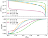Fig. 1. 1D input density profile normalized by the core density and mass profile of each component of the twin binary systems studied in this article. The upper panel corresponds to the stellar density profile while the bottom panel corresponds the mass profile normalized by the total mass of each star.

Two groups of models can be distinguished in Fig. 1: models with high or low envelope mass fractions. While massive and solar-like stars have a nearly negligible envelope mass, for low-mass and red giant branch (RGB) stars, most of their mass is located in their envelope. In particular, the mass of about 80% of our RGB star is located in the convective envelope, with the transition from the radiative core to the convective envelope located at r/R_1D ∼ 0.05 for this star.

In the following sections, we compare the deformations obtained from the different types of stars presented above with the Roche models and with our new type of models. We then relate those differences directly to their 1D density and mass profiles presented in Fig. 1.

4.3. Surface deformation

The surface deformation of binary stars is directly related to its total potential. In our models, the surface of a star composing the binary system is defined by the equipotential corresponding to the photosphere of our 1D input stellar model in the direction (μ_crit, ϕ_crit), as presented in Sect. 2.3.

Both formulations of the classical Roche model and our refined version give the same deformations at the surface, as the total potentials have the same expressions outside of the star. In order to study the deformation given by the Roche model, we assumed, as done in our models, that the volumetric average radius coincides with the 1D input average radii, meaning that the volume and mass of the models are conserved. Using this property, we could define the surface given by the Roche model with the same criterion as our models. In Fig. 2, the position of the surface as given by the Roche model and our model is compared in the case of the 0.2 M_⊙ star with an orbital separation of 2.8 R_1D. The R_1D denotes the radius of the 1D spherically symmetric model.

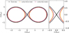Fig. 2. Surface deformation of the twin binary system of our 0.2 M⊙ stars with a separation of 2.8 R1D (corresponding to a period of 2 h and 11 min) as viewed from the side of the system. The black curve corresponds to the Roche lobe of the system, the yellow curve is the surface of each star given by the Roche model while the purple curve corresponds to the surface of each star given by the modelling with MoBiDICT. In this particular case, the filling of the Roche lobes is of 81.7% with each model.

Figure 2 shows a visible difference in surface deformation between our models and the Roche model. To quantify this difference, we introduced a new quantity:

$$\begin{array}{c}\hfill \mathrm{\Delta }R=\frac{R_{\mathrm{s},\mathrm{MoBiDICT}}(\mu =0,\varphi =0)-R_{\mathrm{s},\mathrm{Roche}}(\mu =0,\varphi =0)}{R_{\mathrm{s},\mathrm{Roche}}(\mu =0,\varphi =0)-R_{1\mathrm{D}}}.\end{array}$$(36)

This quantity represents the difference in deformation at the closest point normalised by the deformation between the Roche model and the 1D input model. For the system presented in Fig. 2, this factor is ΔR = 0.368, which means that we have 36.8% more deformation with MoBiDICT than with the Roche model at the closest surface point to the Lagrangian point L1. The difference in surface deformation is a function of the orbital separation between the two components of the binary system. To draw a comparison between the different types of stars, we used the ratio of orbital separation to initial 1D stellar radius a/R_1D as an indicator of the orbital separation with respect to the type of stars in the system.

While we focus on the most distorted region in the rest of this deformation study, Fig. 2 also shows that surface deformation discrepancies appeared at the poles, where our model is more contracted than the Roche model. To study the significance of the modifications to the surface deformation obtained with MoBiDICT for the different types of stars, we computed a grid of deformed models of twin binary systems composed of each stellar type previously presented. For each system, we varied the orbital separation to explore the dependency of the deformation discrepancy to the orbital separation of the components. The results obtained with this grid of models are presented in Fig. 3.

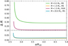Fig. 3. Difference in deformation at the closest point ΔR between Roche and our models as a function of the orbital separation of the components normalized by the input 1D stellar radius a/R1D.

Figure 3 shows that the differences of the deformations are extremely dependent on the type of star studied. In the case of a massive and solar-like MS star, Fig. 3 shows minor discrepancies of surface deformation, even when the stars are close to filling their Roche lobes. At most, the deformation discrepancy reaches 7% before a common envelope or mass transfer phase occurs.

As showed in Fig. 3, RGB stars are significantly more deformed by our modelling (up to ∼35%) than with the Roche model when a/R_1D ≲ 3. Moreover, this discrepancy remains significant even at large a/R_1D with an asymptotic value of ΔR = 0.10.

Finally, we observed that the corrections are the most significant for low-mass stars. As can be seen in Fig. 3, when a/R_1D ≲ 3.5, the Roche model totally underestimates the deformations up to ∼80% just before reaching a common envelope or mass transfer phase.

One would expect that for RGB stars, our new modelling does not significantly change the surface deformation obtained with the Roche model, as RGB stars evolve with a high density contrast between the radiative core and convective envelope, justifying the point-like assumption of the Roche model. In practice with our modelling, we saw that by comparing Figs. 1 and 3, deformation discrepancies are directly related to the 1D mass profiles of each star. Stars with the largest mass fraction in their upper layers are the most impacted by our modelling. In particular, in our RGB model, the low density of the envelope is totally compensated by its significant volume, leading to an envelope mass of about 0.8 M_tot (see Fig. 1). MoBiDICT is necessary to model deformations of close binaries composed of stars with a high envelope mass fraction, such as RGB or low-mass stars.

All the differences previously presented can have a significant impact on the theoretical evolution of binary stars, as mass transfer occurs at higher orbital separation than predicted by the Roche model. Therefore, mass transfers and common envelope phases can occur in earlier system evolutionary stages than with the Roche model, impacting the future evolutionary path of such systems. In that respect, the significant deformation discrepancy found for RGB stars is crucial, as most of the mass transfers are expected to occur during late evolutionary stages, due to the rapid radius inflation resulting from stellar evolution. For example, in the system presented in Fig. 2, a common envelope phase is expected to occur when the orbital period reaches 2 h and 05 min with our modelling, while with the Roche model an orbital period of 2 h is required.

In Sect. 2.4, we mentioned and presented the different readjustments made at the end of each modelling iteration. One of these readjustments, presented in Appendix A, concerns modifying the computation of the system orbital period so that the non-spherical shapes of deformed binaries are taken into account. In the case of low-mass binaries, we saw an approximately 1% increase in the orbital period for a given orbital separation. Compared to the usual uncertainties in the determination of orbital periods, this effect dominates the uncertainties when linking the orbital period of a system to its orbital separation.

4.4. Effective surface gravity

On the observational side, more than having significantly larger deformations than the Roche model, with MoBiDICT the surface effective gravity is directly impacted, as the topology of the total potential is modified. The local brightness of a star as given, for example, in Eq. (26) is proportional to the surface local effective gravity. Therefore, a modification of the total potential topology can directly be seen in the light curves of eclipsing binary systems and impact the derivation of the orbital parameters, for example. As we focus on the surface effective gravity and both our refined Roche model and the classical Roche model give the same result, only one of them is considered in the rest of this section.

In our models, the effective gravity has an integral expression, given in Appendix B, and for the Roche model, the effective gravity is given by |g_eff|=|∇Ψ_tot, Roche|, where Ψ_tot, Roche is given in Sect. 4.1. For the Roche model and our models, Fig. 4 compares the surface effective gravity along the meridian passing by the most distorted point and the poles of the stars for a twin system composed of two 0.2 M_⊙ stars with an orbital separation of 2.8 R_1D.

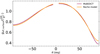Fig. 4. Surface effective gravity of the meridian passing by the most distorted point of the star, its opposite, and the pole. The orange curve corresponds to the surface effective gravity given by the Roche model while the purple curve corresponds to the effective gravity obtained with our modelling. The system modelled here is a twin system composed of two 0.2 M⊙ stars with an orbital separation of 2.8 R1D. The absence of points near θ = 0 is explained by the Gauss-Legendre quadrature method that is not creating any points in this region of our grids. θ > 0 corresponds the direction where the stars are facing each other, while the direction θ < 0 corresponds to the back of the system.

Figure 4 shows that a difference of surface effective gravity exists between the Roche model and our modelling. The most significant g_eff discrepancies are located at the region closest to the L1 point, where we have a normalised the g_eff difference of 12% with respect to the Roche model.

The discrepancies found can be explained by several factors. First, as our models are noticeably more distorted than the Roche model, the surface effective gravity is consequently significantly lower at the surface. To a lesser extent, not correcting the Roche model for the redistribution of mass in the star can impact the surface g_eff.

To summarise the differences obtained, we computed the effective gravity of the grid of models presented in Sect. 4.3 and quantified the differences of surface effective gravity between our models with the quantity Δg_{eff, surface}, defined as

$$\begin{array}{c}\hfill \mathrm{\Delta }{g}_{\mathrm{eff}}=\frac{g_{\mathrm{eff},\mathrm{MoBiDICT}}(\mu =0,\varphi =0)-g_{\mathrm{eff},\mathrm{Roche}}(\mu =0,\varphi =0)}{G{M}_{\star }/R_{1\mathrm{D}}^2}.\end{array}$$(37)

In Fig. 5, we summarise all the differences of surface effective gravity for the twin binary systems presented in Sect. 4.3 and for a wide diversity of orbital separations. Figure 5 shows the same overall results as Fig. 3. The models with most surface deformation discrepancies compared to the Roche model are the same models exhibiting the stronger surface effective gravity differences. In particular, Fig. 5 shows that higher discrepancies of g_eff are found for the RGB and low-mass stars when a/R_1D ≲ 3.2, as the other MS stars have limited corrections from our modelling.

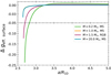Fig. 5. Difference of surface effective gravity of the most distorted point as a function of orbital separation for the four types of twin binaries studied.

For the interpretation of observations, the modifications of g_eff can, in theory, strongly impact the light curves of close binary systems, as the local effective temperature of a star is directly proportional to the surface effective gravity. With our modelling, we expected that a star would appear colder than with the Roche model. In particular, the equator is the region that would appear noticeably colder and thus redder. To confirm these considerations, simulations of binary light curves using models from MoBiDICT have to be developed.

4.5. Structural deformation

The last point of comparison between the Roche model and our models is the structural deformation of the bodies composing the binary system. For this study, we compared the classical Roche model, our refined Roche model, and the model obtained through MoBiDICT. The structural discrepancy can be first seen in the total potential Ψ_tot and the effective gravity g_eff, as these quantities define the structural properties of our models. Figure 6 illustrates the evolution of Ψ_tot and g_eff in a particular direction, the axis linking the centre of both stars, and the system centre of mass for the 0.2 M_⊙ stars with an orbital separation of a = 2.8R_1D.

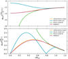Fig. 6. Normalized total potential Ψtot and effective gravity geff in the stellar interior along the axis joining the centre of the two stars. The system studied here is a twin binary system composed of 0.2 M⊙ stars with an orbital separation of a = 2.8R1D. The blue and green curves are corresponding to the classical Roche model while the orange and violet curves are respectively our refined Roche model and our new types of models.

Figure 6 illustrates the limitations of Roche models to study the stellar structure of deformed binaries. Classical ways of computing the Roche potential (Eqs. (33) and (34)) are inaccurate when modelling the stellar interior, while the surface properties are well reproduced. In addition, Fig. 6 shows that our refined Roche model is particularity accurate in obtaining both Ψ_tot and g_eff, even if discrepancies can be seen in the entire star.

In the work of Fabry et al. (2022), the potential used to compute the f_p and f_T factors, Eqs. (24) and (30), corresponds to the green curve in Fig. 6. However, with assumptions on its derivative, the corresponding effective gravity used is the expression given by our refined Roche model. Even if the effective gravity is correct and able to obtain some f_p and f_T, the potential used to identify the equipotentials on which the average quantities are computed is not representative of the stellar deformed structure. Corrections can therefore be expected on the averaged internal quantities f_p and f_T in Fabry et al. (2022), for example.

To quantify the structural differences on the entire stellar structure, we used the coefficients f_p and f_T presented in Sect. 3. As our work considers the entire deformed structure as a function of the radius, we limited our study to twin binary systems composed of our four types of stars presented in Sect. 4.2 with an orbital separation of 2.7 R_1D. The resulting f_p and f_T obtained with the different models are respectively illustrated in Figs. 7 and 8. As classical expressions of the Roche model lead to unphysical results on the majority of the stellar structure, f_p and f_T were not studied for these models.

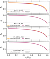Fig. 7. Evolution of fp as a function of the radius of stars in twin binary systems for the different models compared. From top to bottom, each panel respectively represents fp for the 0.2, 1.0, 1.5 and 20.0 M⊙ stars in twin binary systems. The orange curves are the results with our refined Roche model while the purple curves are the results from MoBiDICT.

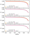Fig. 8. Evolution of fT as a function of the radius of stars in twin binary systems for the different models compared. From top to bottom, each panel respectively represents fT for the 0.2, 1.0, 1.5 and 20.0 M⊙ stars in twin binary systems. The orange curves are the results with our refined Roche model while the purple curves are the results from MoBiDICT.

Figures 7 and 8 show that models with the most deformation discrepancies with respect to the refined Roche model are also the models with the highest f_p and f_T differences. This structural difference can mainly be seen in the upper layers of the 0.2 and 1.5 M_⊙ stars, as these bodies have the largest deformation discrepancies as compared to the Roche model. Moreover, in the case of the 0.2 M_⊙ binary system, a discrepancy in the entire structure can be seen. By predicting a lower f_p and f_T, our modelling impacts the structure of binary stars. Combined with the discrepancies seen in deformations, our modelling can significantly alter the evolutionary path of binary systems. Finally, as previously seen, for MS massive and solar-like stars, our modelling does not significantly change their structural depiction.

5. Comparison with perturbative models

The principle of perturbative models is to treat the centrifugal and tidal forces as perturbations of the spherical symmetry by only accounting for the leading terms. The potentials and densities of the models are also projected on a basis of spherical harmonics by only taking the leading order, namely, the ℓ = 0 and ℓ = 2 terms. The objectives of this section are to determine the precision limits to only account for the leading order terms in the spherical projections and to see whether the treatment of deformations by a perturbative approach is justified in the most distorted cases.

In Sect. 5.1, we present the theoretical formulation of the perturbative models. Section 5.2 is dedicated to the exploration of the limitations of the selection of spherical harmonic projections of the gravitational potential, while in Sect. 5.3 we study the limit of the perturbative approach in the treatment of the tidal and centrifugal forces.

5.1. Theoretical formulation of perturbative model

As explained previously, the perturbative models are a class of models treating the centrifugal and tidal forces as a first order perturbation to the spherical symmetry. The gravitational potential is obtained, as in MoBiDICT, through Eq. (11) but only taking in account the first order terms: the ℓ = 0 and ℓ = 2. With this perturbative modelling, the feedback process where the modification of the potential leads to a redistribution of the masses (therefore impacting the potential that requires updating in an iterative process) is not present. Without going through a detailed demonstration of the equations used in the perturbative model, we mention that the assumptions made allowed us to simplify the expression of the deformations that are related to the structural coefficient η_ℓ. These coefficients are linked to the deformations of a star through their definition

$$\begin{array}{c}\hfill {\eta }_{\ell }^m(\overline{r})=\frac{\overline{r}}{r_{\ell }^m(\overline{r})}\frac{\mathrm{d}{r}_{\ell }^m(\overline{r})}{\mathrm{d}\overline{r}},\end{array}$$(38)

where $\overline{r}$ is the average radius of an isobar that is defined as

$$\begin{array}{c}\hfill \overline{r}=\frac{1}{{\displaystyle {\int }_{{\mathrm{\Psi }}_{\mathrm{tot}}}}\mathrm{d}\sigma }{\int }_{{\mathrm{\Psi }}_{\mathrm{tot}}}r(\mu ,\varphi )\mathrm{d}\sigma ,\end{array}$$(39)

and that is different from r_p corresponding to the radius of the sphere with a volume identical to the one under an isobar. The radii of the equipotentials r(μ, ϕ) projected on the spherical harmonics basis are noted as $r_{\mathcal{l}}^m$ and expressed as done in Eq. (9):

$$\begin{array}{c}\hfill r_{\ell }^m(\overline{r})=\frac{1}{\overline{r}}{\displaystyle {\int }_0^1{\int }_0^{\pi }r(\overline{r},\mu ,\varphi )P_{\ell }^m(\mu )cos(m\varphi )\mathrm{d}\varphi \mathrm{d}\mu .}\end{array}$$(40)

The overall deformation of a given point in a model can thus be obtained by projecting back these $r_{\ell }^m(\overline{r})$ on the spherical coordinates basis as follows:

$$\begin{array}{c}\hfill r(\overline{r},\mu ,\varphi )=\overline{r}{\displaystyle \sum _{k=0}^{(\ell -p)/2}{r}_{\ell }^m(\overline{r})P_{\ell }^m(\mu )cos(m\varphi ),}\end{array}$$(41)

with p = 0 if ℓ is even, p = 1 otherwise, and m = 2k + p.

With the coefficient η_ℓ and using a simple integration, $r_{\ell }^m(\overline{r})$ can be obtained, and thus the deformation of a model can be computed. Physically, these coefficient η_ℓ correspond to the structural answer of a body if a perturbative potential is applied. Using simplifications performed in the perturbative approach, η_ℓ become independent from the deformation undergone by a star and are only related to its unperturbed structure. In the perturbative approach, η_ℓ can be obtained by solving the well-known Clairaut-Radau second order differential equation expressed as

$$\begin{array}{c}\hfill \overline{r}\frac{\mathrm{d}{\eta }_{\ell }}{\mathrm{d}\overline{r}}+6\frac{\rho (\overline{r})}{\overline{\rho }(\overline{r})}({\eta }_{\ell }+1)+{\eta }_{\ell }({\eta }_{\ell }-1)=\ell (\ell +1)\end{array}$$(42)

using the boundary conditions

$$\begin{array}{c}\hfill {\eta }_{\ell }(0)=\ell -2.\end{array}$$(43)

To compute the perturbative models, we developed a small feature in MoBiDICT to solve the Clairaut-Radau equation (Eq. (42)) with an order two Rung-Kutta method and using the 1D input stellar models given in this tool.

For comparison with the model obtained with MoBiDICT, we decided to directly compare the η_ℓ of the two models. To obtain these coefficients with our models, we computed the deformations as described in Sect. 2. Then we obtained $\overline{r}$ and projected the deformations on a basis of spherical harmonics (Eq. (40)) to have the $r_{\ell }^m(\overline{r})$ that were used in Eq. (38) to compute the ${\eta }_{\ell }^m(\overline{r})$ coefficients directly given by MoBiDICT. We mention that when using these equations, none of the assumptions of the perturbative approach were made.

5.2. Gravitational potential

One main approximation of perturbative models is to only account for the leading order terms (ℓ = 0 and ℓ = 2) on the projections of the potential and densities. Verifying these assumptions with MoBiDICT is straightforward, as our modelling directly gives the spherical expansion of the gravitational potential of each deformed star as an output of the code. Figure 9 illustrates the gravitational potential projected on the spherical harmonics basis of the twin binary system composed of the 0.2 M_⊙ stars at an orbital distance of a = 2.8R_1D. This is the exact system configuration illustrated in Fig. 2.

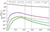Fig. 9. Normalized gravitational potential projected on the spherical harmonics of a star of 0.2 M⊙ in a twin binary system with an orbital separation of a = 2.8R1D. The dotted lines are corresponding to the surface of each star of the system in the direction including the most distorted point of each star and the Lagragian point L1 (μ = 0, ϕ = 0).

Figure 9 illustrates the amplitude hierarchy of gravitational potential spherical terms. As assumed by the perturbative model, the leading order terms are the ℓ = 0 and ℓ = 2 terms. The dipolar term (ℓ = 1) is the next most important term, especially outside of the star, as each spectral term is proportional to r^−ℓ. In these regions, the dipolar term is included in the computation of the tidal potential applied to the opposite star. Neglected by the perturbative model, the ℓ = 1 term is less than one order of magnitude smaller than the ℓ = 2 term, meaning that the tidal force is significantly greater with our models and the assumption to neglect the ℓ = 1 is not justified for the perturbative models in the most distorted cases. The next order terms (ℓ = 3, 4) have amplitudes similar to the ℓ = 1 term inside the star, while they are one order of magnitude smaller than this same dipolar term outside the star.

5.3. Validity of the Clairaut-Radau equation

In this section, we verify the limits of the perturbative approach for close binaries, in particular when the stars undergo high deformations. To compare the different models, as explained in Sect. 5.1, we directly looked at the coefficient η_ℓ obtained through Eq. (42) for perturbative models. With our models, these quantities are computed with a projection on the spherical harmonics of the deformations. More details are given in Sect. 5.1. We also compared these models to our refined Roche model through the same coefficients η_ℓ obtained in the same way as with our models. We focussed our work on the ℓ = 2 term, as this coefficient is assumed by the perturbative model to be the leading contribution to the apsidal motion of a binary system, and it is used, for example, in Rosu et al. (2020, 2022a, b) to constrain the stellar structure. The evolution of η₂ as a function of the average radius is illustrated in Fig. 10 for the extensively studied system of this article, the twin binary system composed of 0.2 M_⊙ stars at an orbital distance of 2.8R_1D.

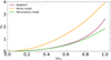Fig. 10. Evolution of η2 as a function of the average radius for the different models studied in this work. The system studied here is a twin binary system composed of two 0.2 M⊙ stars with an orbital distance of 2.8R1D.

Figure 10 illustrates the different significant results from our modelling. First, comparing the Roche model to other models, we observed that both perturbative and MoBiDICT models predict an important difference of η₂ in all the stars. These results can be interpreted as difficulties of the Roche model to precisely depict the stellar deformations. These limitations originate from the assumptions on the stellar gravitational potential.

The second major result illustrated in Fig. 10 is the comparison between our new models and the perturbative models. First, in the less distorted regions of the star (when $\overline{r}<0.5R_{1\mathrm{D}}$), the same results were obtained with the models, indicating that our modelling gives a good depiction of stellar deformation in these regions, as we expected to be in the limit of validity of the perturbative modelling. Then, after $\overline{r}>0.5R_{1\mathrm{D}}$, non-negligible differences between the two models appeared, with discrepancies increasing with $\overline{r}$, as the upper layers of the star are more deformed. These differences can be explained by the limitations of the perturbative approach in these regimes of deformation, while our model is designed to study cases with high stellar deformations.

To study the apsidal motion of a binary system, one would require the apsidal motion constant k₂ that is usually obtained through η₂ evaluated at the surface of the primary star. To study how our new modelling procedure impacts this apsidal motion constant in regard to the twin binary system studied and orbital separation, we introduced a new quantity Δη₂ defined as the difference of η₂ at the stellar surface between our model and the perturbative model. The quantity Δη₂ is expressed as

$$\begin{array}{c}\hfill \mathrm{\Delta }{\eta }_2={\eta }_{2,\mathrm{MoBiDICT}}({\overline{R}}_{\mathrm{s}})-{\eta }_{2,\mathrm{pert}.}({\overline{R}}_{\mathrm{s}}).\end{array}$$(44)

The comparison of Δη₂ from the grid of the twin binary models presented in Sect. 4.2, as a function of their orbital separation, is illustrated in Fig. 11.

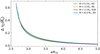Fig. 11. Evolution of the surface Δη2 for different types of stars composing the binaries and with different orbital separation.

Figure 11 illustrates that the differences of η₂ between the perturbative and MoBiDICT models are almost independent from the type of star composing the binary system and only dependent on the orbital separation of the components. Significant differences of surface η₂ can only be seen in the most distorted cases, when a < 5R_1D. Otherwise, the perturbative treatment of the tidal and centrifugal forces is justified to compute η₂. We expect the differences we found to directly impact the apsidal motion computation, resulting in corrections to apsidal motion constant k₂ and adding k₁ constant to account for neglected dipolar terms. The impact of our improved modelling on apsidal motion will be more deeply investigated in a forthcoming article.

6. Conclusion

In this work, we developed a new tool called MoBiDICT to compute 3D static models of close synchronised binaries in hydrostatic equilibrium in a non-perturbative way. Sections 2 and 3 were respectively dedicated to giving a technical description of this code and presented the post-treatment done in our models to couple, in the future, MoBiDICT to classical 1D evolution codes. We then compared our new type of modelling to classical models, namely, the Roche and perturbative models.

First, for the Roche model, our study showed in Sect. 4 that the differences of deformation mainly arise in very close binaries (when a < 5R_1D). The discrepancies are significant for low-mass and RGB stars in twin binary systems where the deformation differences can reach, at most, 80% for our 0.2 M_⊙ stars. Massive and solar-like MS stars are less distorted, with a difference of 7% at most. The envelope mass is the key parameter controlling these deformation discrepancies. Stellar models with the largest envelope masses compared to the total mass were observed to be the most modified by MoBiDICT. All the quantities studied were impacted by this difference. In particular, significant changes of the surface effective gravity were seen, which directly affected gravity darkening and thus the interpretation of the observations of such stars. In the lower deformation regime, the Roche model provides a good approximation of the stellar surface properties, although we would not favour using Roche to study the structural properties of stars.

The discrepancies with respect to the perturbative approach were discussed in Sect. 5. Our work showed that the assumption of the perturbative model to only account for the leading terms of the projected gravitational potential (ℓ = 0 and ℓ = 2) is not justified in the high-distortion cases (when a < 5R_1D). In particular, the dipolar term (ℓ = 1) represented 31% of the quadrupolar term (ℓ = 2) outside of the studied star and 14% at its surface. In addition, we showed that in such regimes of distortion, the perturbative approach reaches its limit and significant deformation discrepancies can be seen, particularly in the upper layers of the stars (when r > 0.5R_1D). These differences of deformation were seen through the quantity η₂ that was evaluated at the surface to estimate the apsidal motion of binary systems. In such a distortion regime, the theoretical apsidal motion from the quadrupolar term is generally considerably underestimated, and an additional term from the dipolar component is likely to arise. In the least distorted regime (a > 5R_1D), the perturbative approach remains valid, and accurate η₂ values were obtained.

A few conclusions can be drawn from our work. First, in least distorted regimes, the classical modelling methods for binaries are valid, at the surface for the Roche model and in the entire structure for perturbative models. In the most distorted regimes, however, both the perturbative and Roche models fail to describe the structural and surface properties of stars with high envelope masses. In particular, significant deformation discrepancies were observed for low-mass stars, in agreement with the results of Landin et al. (2009). Our work highlights the necessity of non-perturbative modelling to study close binary interactions and evolution, as mass transfer is expected to occur earlier in the lifetime of a system under our modelling approach. In that regard, deformation discrepancies found for RGB stars significantly facilitate mass transfer occurrence during a stellar evolutionary phase already believed to be a source of mass transfer.

Our method, while effective in modelling highly distorted cases, has demonstrated limitations when deformations are extremely weak. Specifically, we observed numerical noise arising from higher spherical orders of the potential and densities that impact the derived η_ℓ. To address these issues, we plan to implement a coupling of MoBiDICT, in the least distorted regions, to a refined perturbative approach accounting for all the spherical orders and for terms of the tidal and centrifugal potential that are usually neglected. The advantage of this new form of the perturbative model is the possibility to study solid-body non-synchronised systems that are also easily generalised in MoBiDICT. All these modifications will be the subject of a forthcoming article.

Acknowledgments

The authors are thanking the anonymous referee for his/her constructive comments. L.F was supported by the Fonds de la Recherche Scientifique FNRS as a Reaserch Fellow. The authors would like to thank Martin Farnir from “Psychedelic Kiss Designs” for his help in finding our code name and designing MoBiDICT’s logo.

References

Appendix A: Verification of Kepler’s third law

In this section, we show the system of equations solved at the end of each modelling iteration in order to readjust the centre of mass and the orbital period of our models. We consider an arbitrary synchronised binary system with an orbital separation a, an orbital rotation rate Ω_⋆, and a centre of mass noted CM. This system can be illustrated as in Fig. A.1.

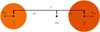Fig. A.1. Schema of an arbitrary chosen binary system composed of two stars with different masses. a1 and a2 are the orbital separation of respectively the primary and secondary star from the centre of mass. ${\widehat{e}}_{{\mathrm{x}}_1}$ and ${\widehat{e}}_{{\mathrm{x}}_2}$ are the unit vectors of the x1 and x2 direction considered in this problem.

The orbital separation of the system a is a constant of the model. Thus, the centre of each star is at the dynamical equilibrium, meaning that the sum of the gravitational, tidal, and centrifugal forces is null in their centre. Mathematically this condition is expressed as

$$\begin{array}{c}\hfill \{\begin{array}{c}{lim}_{{\mathrm{x}}_1\to 0}\frac{\partial {\mathrm{\Psi }}_1}{\partial {\mathrm{x}}_1}+\frac{\partial {\mathrm{\Psi }}_2}{\partial {\mathrm{x}}_1}={\mathrm{\Omega }}_{\star }^2{x}_{\mathrm{CM}}a\hfill \\ \hfill \\ {lim}_{{\mathrm{x}}_2\to 0}\frac{\partial {\mathrm{\Psi }}_1}{\partial {\mathrm{x}}_2}+\frac{\partial {\mathrm{\Psi }}_2}{\partial {\mathrm{x}}_2}={\mathrm{\Omega }}_{\star }^2(1-x_{\mathrm{CM}})a\hfill \end{array},\end{array}$$(A.1)

where x_CM is defined as a₁/a.

The system given in Eq. A.1 can be summed and rewritten as

$$\begin{array}{c}\hfill \{\begin{array}{c}{lim}_{{\mathrm{x}}_1\to 0}\frac{\partial {\mathrm{\Psi }}_1}{\partial {\mathrm{x}}_1}+\frac{\partial {\mathrm{\Psi }}_2}{\partial {\mathrm{x}}_1}={\mathrm{\Omega }}_{\star }^2{x}_{\mathrm{CM}}a\hfill \\ \hfill \\ {lim}_{{\mathrm{x}}_1\to 0}(\frac{\partial {\mathrm{\Psi }}_1}{\partial {\mathrm{x}}_1}+\frac{\partial {\mathrm{\Psi }}_2}{\partial {\mathrm{x}}_1})+{lim}_{{\mathrm{x}}_2\to 0}(\frac{\partial {\mathrm{\Psi }}_1}{\partial {\mathrm{x}}_2}+\frac{\partial {\mathrm{\Psi }}_2}{\partial {\mathrm{x}}_2})={\mathrm{\Omega }}_{\star }^{2}a\hfill \end{array}.\end{array}$$(A.2)

The second equation of this system can be solved with MoBiDICT to obtain the ${\mathrm{\Omega }}_{\star }^2$ necessary to maintain the orbital separation of the binary system. Having ${\mathrm{\Omega }}_{\star }^2$, the first equation can be solved to obtain the new position of the centre of mass of the system while accounting for the redistribution of mass in the stars.

Appendix B: Expression of the effective gravity

In this section, we develop the expression of the effective gravity used in MoBiDICT.

The effective gravity is a vector defined by

$$\begin{array}{c}\hfill \begin{array}{cc}\hfill {\mathbf{g}}_{\mathrm{eff}}& =-\mathbf{\nabla }{\mathrm{\Psi }}_{\mathrm{tot}}\hfill \\ \hfill & =-\mathbf{\nabla }({\mathrm{\Psi }}_1-{\mathrm{\Psi }}_2-{\mathrm{\Psi }}_{\mathrm{centri}})\hfill \\ \hfill & =-(g_{\mathrm{eff},r};g_{\mathrm{eff},\mu };g_{\mathrm{eff},\varphi }),\hfill \end{array}\end{array}$$(B.1)

with each component of a given primary star noted as ‘star 1’ expressed as

$$\begin{array}{cc}\hfill g_{\mathrm{eff},r,1}& =\frac{\partial {\mathrm{\Psi }}_{\mathrm{tot},1}}{\partial r_1}=\frac{\partial {\mathrm{\Psi }}_1}{\partial r_1}+\frac{\partial {\mathrm{\Psi }}_2}{\partial r_1}+\frac{\partial {\mathrm{\Psi }}_{\mathrm{centri}}}{\partial r_1},\hfill \end{array}$$(B.2)

$$\begin{array}{cc}\hfill g_{\mathrm{eff},\mu ,1}& =\frac{1}{r_1}\frac{\partial {\mathrm{\Psi }}_{\mathrm{tot},1}}{\partial {\theta }_1}=\frac{1}{r_1}(\frac{\partial {\mathrm{\Psi }}_1}{\partial {\theta }_1}+\frac{\partial {\mathrm{\Psi }}_2}{\partial {\theta }_1}+\frac{\partial {\mathrm{\Psi }}_{\mathrm{centri}}}{\partial {\theta }_1}),\hfill \end{array}$$(B.3)

$$\begin{array}{cc}\hfill g_{\mathrm{eff},\varphi ,1}& =\frac{1}{r_{1}sin({\varphi }_1)}\frac{\partial {\mathrm{\Psi }}_{\mathrm{tot},1}}{\partial {\varphi }_1}\hfill \\ \hfill & =\frac{1}{r_{1}sin({\theta }_1)}(\frac{\partial {\mathrm{\Psi }}_1}{\partial {\varphi }_1}+\frac{\partial {\mathrm{\Psi }}_2}{\partial {\varphi }_1}+\frac{\partial {\mathrm{\Psi }}_{\mathrm{centri}}}{\partial {\varphi }_1}).\hfill \end{array}$$(B.4)

In this case, all the necessary quantities are partial derivatives of solutions to differential equations that have integral representations. Consequently, numerical methods are not required to perform the derivatives of the potentials. The contribution to effective gravity from gravitational potential of the primary star is given by

$$\begin{array}{cc}\hfill \frac{\partial {\mathrm{\Psi }}_1}{\partial r_1}& ={\displaystyle \sum _{\ell ,m}{P}_{\ell }^m({\mu }_1)cos(m{\varphi }_1)\frac{\partial {\mathrm{\Psi }}_{1,\ell }^m}{\partial r_1}}\hfill \\ \hfill & ={\displaystyle \sum _{\ell ,m}{P}_{\ell }^m({\mu }_1)cos(m{\varphi }_1)({\mathrm{\Psi }}_{1,\ell }^m\frac{\ell }{r_1}+r_1^{-(\ell +2)}{\int }_0^{r_1}{r}_1^{\prime \ell +2}{\rho }_{1,\ell }^m(r_1^{\prime })\mathrm{d}{r}^{\prime }),}\hfill \end{array}$$(B.5)

$$\begin{array}{c}\hfill \frac{\partial {\mathrm{\Psi }}_1}{\partial {\theta }_1}=-{\displaystyle \sum _{\ell ,m}{\mathrm{\Psi }}_{1,\ell }^m(r_1)cos(m{\varphi }_1)\frac{\partial P_{\ell }^m({\mu }_1)}{\partial {\mu }_1}sin({\theta }_1),}\end{array}$$(B.6)

$$\begin{array}{c}\hfill \frac{\partial {\mathrm{\Psi }}_1}{\partial {\varphi }_1}=-{\displaystyle \sum _{\ell ,m}{\mathrm{\Psi }}_{1,\ell }^m(r_1)msin(m{\varphi }_1)P_{\ell }^m({\mu }_1).}\end{array}$$(B.7)

The contribution from centrifugal force is expressed as

$$\begin{array}{cc}\hfill \mathbf{\nabla }{\mathrm{\Psi }}_{\mathrm{centri}}& ={\mathrm{\Omega }}_{\star }^2(x_{\mathrm{CM}}-rsin(\theta )cos(\varphi ))\left[\begin{array}{c}sin(\theta )cos(\varphi )\hfill \\ rcos(\theta )cos(\varphi )\hfill \\ -rsin(\theta )sin(\varphi )\hfill \end{array}\right]\hfill \\ \hfill & -{\mathrm{\Omega }}_{\star }^2(rsin(\theta )sin(\varphi ))\left[\begin{array}{c}sin(\theta )sin(\varphi )\hfill \\ rcos(\theta )sin(\varphi )\hfill \\ rsin(\theta )cos(\varphi )\hfill \end{array}\right],\hfill \end{array}$$(B.8)

Finally, the gravitational contribution originating from the companion is written as

$$\begin{array}{c}\hfill \left[\begin{array}{c}\frac{\partial {\mathrm{\Psi }}_2}{\partial r_1}\hfill \\ \frac{\partial {\mathrm{\Psi }}_2}{\partial {\theta }_1}\hfill \\ \frac{\partial {\mathrm{\Psi }}_2}{\partial {\varphi }_1}\hfill \end{array}\right]=-{\mathbf{J}}^{-1}{\displaystyle \sum _{\ell ,m}}{\mathrm{\Psi }}_{2,\ell }^m(R_{0,2}){\left(\frac{R_{0,2}}{r_2}\right)}^{\ell +1}\left[\begin{array}{c}\frac{\ell +1}{r_2}{P}_{\ell }^m({\mu }_2)cos(m{\varphi }_2)\hfill \\ \frac{\partial P_{\ell }^m({\mu }_2)}{\partial {\mu }_2}sin({\theta }_2)cos(m{\varphi }_2)\hfill \\ P_{\ell }^m({\mu }_2)msin(m{\varphi }_2)\hfill \end{array}\right],\end{array}$$(B.9)

where J⁻¹ is the inverse of the Jacobian matrix taken between the system of coordinates of our primary and secondary star, and expressed as

$$\begin{array}{c}\hfill {\mathbf{J}}^{-1}=\left[\begin{array}{c}\frac{\partial r_2}{\partial r_1}\frac{\partial {\theta }_2}{\partial r_1}\frac{\partial {\varphi }_2}{\partial r_1}\hfill \\ \frac{\partial r_2}{\partial {\theta }_1}\frac{\partial {\theta }_2}{\partial {\theta }_1}\frac{\partial {\varphi }_2}{\partial {\theta }_1}\hfill \\ \frac{\partial r_2}{\partial {\varphi }_1}\frac{\partial {\theta }_2}{\partial {\varphi }_1}\frac{\partial {\varphi }_2}{\partial {\varphi }_1}\hfill \end{array}\right].\end{array}$$(B.10)

The norm of the effective gravity is simply given by

$$\begin{array}{c}\hfill |{\mathbf{g}}_{\mathrm{eff}}|={(g_{\mathrm{eff},r,1}^2+g_{\mathrm{eff},\mu ,1}^2+g_{\mathrm{eff},\varphi ,1}^2)}^{1/2}.\end{array}$$(B.11)

All Tables

All Figures

	Fig. 1. 1D input density profile normalized by the core density and mass profile of each component of the twin binary systems studied in this article. The upper panel corresponds to the stellar density profile while the bottom panel corresponds the mass profile normalized by the total mass of each star.
In the text

Fig. 2. Surface deformation of the twin binary system of our 0.2 M⊙ stars with a separation of 2.8 R1D (corresponding to a period of 2 h and 11 min) as viewed from the side of the system. The black curve corresponds to the Roche lobe of the system, the yellow curve is the surface of each star given by the Roche model while the purple curve corresponds to the surface of each star given by the modelling with MoBiDICT. In this particular case, the filling of the Roche lobes is of 81.7% with each model.

In the text

	Fig. 3. Difference in deformation at the closest point ΔR between Roche and our models as a function of the orbital separation of the components normalized by the input 1D stellar radius a/R1D.
In the text

Fig. 4. Surface effective gravity of the meridian passing by the most distorted point of the star, its opposite, and the pole. The orange curve corresponds to the surface effective gravity given by the Roche model while the purple curve corresponds to the effective gravity obtained with our modelling. The system modelled here is a twin system composed of two 0.2 M⊙ stars with an orbital separation of 2.8 R1D. The absence of points near θ = 0 is explained by the Gauss-Legendre quadrature method that is not creating any points in this region of our grids. θ > 0 corresponds the direction where the stars are facing each other, while the direction θ < 0 corresponds to the back of the system.

In the text

	Fig. 5. Difference of surface effective gravity of the most distorted point as a function of orbital separation for the four types of twin binaries studied.
In the text

Fig. 6. Normalized total potential Ψtot and effective gravity geff in the stellar interior along the axis joining the centre of the two stars. The system studied here is a twin binary system composed of 0.2 M⊙ stars with an orbital separation of a = 2.8R1D. The blue and green curves are corresponding to the classical Roche model while the orange and violet curves are respectively our refined Roche model and our new types of models.

In the text

	Fig. 7. Evolution of fp as a function of the radius of stars in twin binary systems for the different models compared. From top to bottom, each panel respectively represents fp for the 0.2, 1.0, 1.5 and 20.0 M⊙ stars in twin binary systems. The orange curves are the results with our refined Roche model while the purple curves are the results from MoBiDICT.
In the text

	Fig. 8. Evolution of fT as a function of the radius of stars in twin binary systems for the different models compared. From top to bottom, each panel respectively represents fT for the 0.2, 1.0, 1.5 and 20.0 M⊙ stars in twin binary systems. The orange curves are the results with our refined Roche model while the purple curves are the results from MoBiDICT.
In the text

	Fig. 9. Normalized gravitational potential projected on the spherical harmonics of a star of 0.2 M⊙ in a twin binary system with an orbital separation of a = 2.8R1D. The dotted lines are corresponding to the surface of each star of the system in the direction including the most distorted point of each star and the Lagragian point L1 (μ = 0, ϕ = 0).
In the text

	Fig. 10. Evolution of η2 as a function of the average radius for the different models studied in this work. The system studied here is a twin binary system composed of two 0.2 M⊙ stars with an orbital distance of 2.8R1D.
In the text

	Fig. 11. Evolution of the surface Δη2 for different types of stars composing the binaries and with different orbital separation.
In the text

	Fig. A.1. Schema of an arbitrary chosen binary system composed of two stars with different masses. a1 and a2 are the orbital separation of respectively the primary and secondary star from the centre of mass. ${\widehat{e}}_{{\mathrm{x}}_1}$ and ${\widehat{e}}_{{\mathrm{x}}_2}$ are the unit vectors of the x1 and x2 direction considered in this problem.
In the text

References

- Aharonian, F., Akhperjanian, A. G., Aye, K. M., et al. 2005, A&A, 442, 1 [NASA ADS] [CrossRef] [EDP Sciences] [Google Scholar]
- Fabry, M., Marchant, P., & Sana, H. 2022, A&A, 661, A123 [NASA ADS] [CrossRef] [EDP Sciences] [Google Scholar]
- Fitzpatrick, R. 2012, An Introduction to Celestial Mechanics (Cambridge: Cambridge University Press) [CrossRef] [Google Scholar]
- Gaia Collaboration 2022, VizieR Online Data Catalog: I/357 [Google Scholar]
- Gaia Collaboration (Brown, A. G. A., et al.) 2021, A&A, 649, A1 [NASA ADS] [CrossRef] [EDP Sciences] [Google Scholar]
- Han, Z., Podsiadlowski, P., Maxted, P. F. L., Marsh, T. R., & Ivanova, N. 2002, MNRAS, 336, 449 [Google Scholar]
- Han, Z., Podsiadlowski, P., Maxted, P. F. L., & Marsh, T. R. 2003, MNRAS, 341, 669 [NASA ADS] [CrossRef] [Google Scholar]
- Heber, U. 2009, ARA&A, 47, 211 [Google Scholar]
- Houdayer, P. S., & Reese, D. R. 2023, A&A, 675, A181 [NASA ADS] [CrossRef] [EDP Sciences] [Google Scholar]
- Hurley, J. R., Tout, C. A., & Pols, O. R. 2002, MNRAS, 329, 897 [Google Scholar]
- Kippenhahn, R., & Thomas, H. C. 1970, in Stellar Rotation, IAU Colloq., 4, 20 [NASA ADS] [CrossRef] [Google Scholar]
- Kopal, Z. 1959, Close Binary Systems (London: Chapman& Hall) [Google Scholar]
- Kopal, Z. 1978, Dynamics of Close Binary Systems (Dordrecht: Reidel) [Google Scholar]
- Landin, N. R., Mendes, L. T. S., & Vaz, L. P. R. 2009, A&A, 494, 209 [NASA ADS] [CrossRef] [EDP Sciences] [Google Scholar]
- Manchon, L. 2021, Ph.D. Thesis, Université Paris-Saclay, France [Google Scholar]
- Meynet, G., & Maeder, A. 1997, A&A, 321, 465 [NASA ADS] [Google Scholar]
- Palate, M., Rauw, G., & Mahy, L. 2013, Cent. Eur. Astrophys. Bull., 37, 311 [Google Scholar]
- Patterson, J. 1984, ApJS, 54, 443 [NASA ADS] [CrossRef] [Google Scholar]
- Price-Whelan, A. M., Hogg, D. W., Rix, H.-W., et al. 2018, AJ, 156, 18 [Google Scholar]
- Prša, A. 2018, Modeling and Analysis of Eclipsing Binary Stars; The Theory and Design Principles of PHOEBE (Bristol: IOP Publishing) [Google Scholar]
- Rosu, S., Noels, A., Dupret, M. A., et al. 2020, A&A, 642, A221 [EDP Sciences] [Google Scholar]
- Rosu, S., Rauw, G., Farnir, M., Dupret, M. A., & Noels, A. 2022a, A&A, 660, A120 [NASA ADS] [CrossRef] [EDP Sciences] [Google Scholar]
- Rosu, S., Rauw, G., Nazé, Y., Gosset, E., & Sterken, C. 2022b, A&A, 664, A98 [NASA ADS] [CrossRef] [EDP Sciences] [Google Scholar]
- Roxburgh, I. W. 2004, A&A, 428, 171 [NASA ADS] [CrossRef] [EDP Sciences] [Google Scholar]
- Roxburgh, I. W. 2006, A&A, 454, 883 [NASA ADS] [CrossRef] [EDP Sciences] [Google Scholar]
- Sana, H., & Evans, C. J. 2011, IAU Symp., 272, 474 [Google Scholar]
- Sana, H., de Mink, S. E., de Koter, A., et al. 2012, Science, 337, 444 [Google Scholar]
- Sana, H., de Koter, A., de Mink, S. E., et al. 2013, A&A, 550, A107 [NASA ADS] [CrossRef] [EDP Sciences] [Google Scholar]
- Sana, H., Le Bouquin, J. B., Lacour, S., et al. 2014, ApJS, 215, 15 [Google Scholar]
- Savonije, G. J. 1978, A&A, 62, 317 [NASA ADS] [Google Scholar]
- Scuflaire, R., Théado, S., Montalbán, J., et al. 2008, ApSS, 316, 83 [NASA ADS] [Google Scholar]
- Siess, L., Izzard, R. G., Davis, P. J., & Deschamps, R. 2013, A&A, 550, A100 [NASA ADS] [CrossRef] [EDP Sciences] [Google Scholar]
- Slawson, R. W., Prša, A., Welsh, W. F., et al. 2011, AJ, 142, 160 [Google Scholar]