| Issue |
A&A
Volume 676, August 2023
|
|
|---|---|---|
| Article Number | A132 | |
| Number of page(s) | 14 | |
| Section | Interstellar and circumstellar matter | |
| DOI | https://doi.org/10.1051/0004-6361/202244594 | |
| Published online | 23 August 2023 | |
Dark dust
III. The high-quality single-cloud reddening curve sample: Scrutinizing extinction curves in the Milky Way★
1
European Southern Observatory,
Karl-Schwarzschild-Str. 2,
85748
Garching, Germany
e-mail: This email address is being protected from spambots. You need JavaScript enabled to view it.
2
European Southern Observatory,
Alonso de Cordova 3107,
Vitacura, Santiago, Chile
3
UK Astronomy Technology Centre, Royal Observatory, Blackford Hill,
Edinburgh
EH9 3HJ,
UK
4
Materials Spectroscopy Laboratory, University of Rzeszów,
Pigonia 1 Street,
35-310,
Rzeszów, Poland
5
Space Telescope Science Institute,
3700 San Martin Drive,
Baltimore, MD
21218,
USA
6
Ruhr University Bochum, Faculty of Physics and Astronomy, Astronomical Institute (AIRUB),
44780
Bochum, Germany
7
Universidad Católica del Norte, Instituto de Astronomía,
Avenida Angamos 0610,
Antofagasta, Chile
8
Nicolaus Copernicus Astronomical Center, Polish Academy of Sciences,
Bartycka 18,
00-716
Warszawa, Poland
Received:
25
July
2022
Accepted:
1
July
2023
Abstract
The nature of dust in the diffuse interstellar medium can be best investigated by means of reddening curves where only a single interstellar cloud lies between the observer and the background source. Published reddening curves often suffer from various systematic uncertainties. We merged a sample of 820 reddening curves of stars for which both FORS2 polarization spectra and UVES highresolution spectra are available. The resulting 111 sightlines towards OB-type stars have 175 reddening curves. For these stars, we derived their spectral-type from the UVES high-resolution spectroscopy. To obtain high-quality reddening curves, we excluded stars with composite spectra in the IUE/FUSE data due to multiple stellar systems. Likewise, we omitted stars that have uncertain spectral-type designations or stars with photometric variability. We neglected stars that show inconsistent parallaxes when comparing data releases two and three from Gaia. Finally, we identified stars that show differences in the space- and ground-based-derived reddening curves between 0.28 µm and the U band or in RV. In total, we find 53 stars with one or more reddening curves passing the rejection criteria. This provides the highest-quality Milky Way reddening curve sample available today. Averaging the curves from our high-quality sample, we find RV = 3.1 ± 0.4, confirming previous estimates. A future paper in this series will use the current sample of precise reddening curves and combine them with polarization data to study the properties of dark dust.
Key words: dust, extinction / ISM: clouds / stars: early-type
Curves of Fig. 9 are only available at the CDS via anonymous ftp to cdsarc.cds.unistra.fr (130.79.128.5) or via https://cdsarc.cds.unistra.fr/viz-bin/cat/J/A+A/676/A132
© The Authors 2023
 Open Access article, published by EDP Sciences, under the terms of the Creative Commons Attribution License (https://creativecommons.org/licenses/by/4.0), which permits unrestricted use, distribution, and reproduction in any medium, provided the original work is properly cited.
This article is published in open access under the Subscribe to Open model. This email address is being protected from spambots. You need JavaScript enabled to view it. to support open access publication.
1 Dust in the interstellar medium
The disc of our Galaxy, as well as of other spiral galaxies, is filled with the interstellar medium (ISM), consisting of gas, molecules, and dust grains. The ISM is clumpy (Dickey & Lockman 1990; Meyer & Blades 1996), and covers a wide range of temperatures and densities (McKee & Ostriker 1977); based on the latter parameter, one may distinguish three categories – diffuse, translucent, and dense clouds.
Dense clouds are typically star-forming regions, where the high extinction (AV > 5 mag) generally impedes optical observations of embedded stars. Therefore, this component of the ISM is best analysed at infrared and microwave wavelengths (Binder & Povich 2018). Translucent clouds, in contrast, offer the possibility to study the ISM optically via photometric and spectroscopic observations of stars, shining through the material at a moderate density of AV < 3 mag (Snow & McCall 2006). The disadvantage here is that in the majority of cases several clouds are present along a single sightline – an effect that increases with stellar distance. Likewise, there is the diffuse medium which contributes to the extinction along the sight-line (Li & Draine 2001). Furthermore, translucent clouds show striking differences in their chemical composition and physical parameters as witnessed by varying intensity ratios of spectral lines or bands.
The study of the ISM has two origins: Firstly, interstellar gas and dust were discovered by chance during photometric and spectroscopic observations of stars by Hartmann (1904) and Heger (1922), revealing that the precise knowledge of both the interstellar lines and the amount of dust along the sightline were crucial for the interpretation of stellar spectra and photometric data. Secondly, Spitzer (1978) recognized the fundamental role of the ISM in the process of star and planet formation.
After the detection of interstellar dust nearly 100 years ago (Trumpler 1930), it was learned soon after how to compare the spectral energy distribution of unreddened stars with those of reddened stars (see Sect. 3) to quantify the wavelength-dependant reddening by dust grains – leading to the famous extinction curve. Its normalization RV = AV/E(B – V) – the ratio of total-to-selective extinction – was further treated like a constant of nature with a value of RV ~ 3.1. Therefore, early model fits of the extinction curve led to fairly simple dust models with a power-law grain-size distribution of silicate and graphite grains. Only photometric studies, some decades later, of stars in dense, star-forming clouds revealed RV values of up to five, suggesting substantial grain growths – either by coagulation and/or by the formation of mantles (Mathis & Wallenhorst 1981). Furthermore, polycyclic armoatic hydrocarbons were detected by IR spectroscopy in the ISM by Allamandola et al. (1989) and Bouwman et al. (2001). Nevertheless, the RV value kept its importance and was suggested to be the only parameter that determines the extinction law (Cardelli et al. 1989).
In the present work, we readdress the issue of reddening curves by analysing and completing published data. The ideal set of data required to determine a reddening curve would be a spectroscopically accurately classified star, with data from the UV to IR, at a reliable Gaia (Gaia Collaboration 2016) distance and with a single translucent cloud along the sightline. Unfortunately, such cases are rare, calling into question many published reddening curves. For example, due to their large distances, light from OB-type stars typically passes through several intervening clouds (Welty et al. 1994). Therefore, the observed extinction curves for different sightlines are usually quite similar to each other, simulating a similar RV value. However, they are ill-defined averages in the sense that measurements of single-cloud sightlines with similar chemical compositions should preferentially be used when studying the physical properties of dust or the magnetic field direction when extracted from the optical polarization angle.
To improve the sample from which precise reddening curves can be derived, we selected sightlines where spectra show interstellar atomic lines or features of simple radicals, dominated by only one Doppler component. Such single-cloud sightlines can be interpreted in terms of better defined physical conditions. Furthermore, we focus on OB-type stars with known trigonometric parallaxes from Gaia. For future observations, it seems important to select and scrutinize all cases from the extensive catalogues by Valencic et al. (2004), Fitzpatrick & Massa (2007), and Gordon et al. (2009).
This paper is the third in a series concerned with dark dust, which is composed of very large and very cold grains in the ISM. The first paper, Siebenmorgen et al. (2020), presented initial results derived from distance unification and the second, Siebenmorgen (2023), presented a dust model for the general ISM, which was tested against the contemporary set of observational constraints (Ysard 2020; Hensley & Draine 2021). The current paper presents a high-quality sample of reddening curves obtained from the literature as needed for detailed modelling of particular sightlines. It is laid out as follows: Sect. 2 presents the sample of sightlines, with many of them being dominated by single interstellar lines. Section 3 describes how interstellar reddening curves are calculated and discusses the impact of binarity and uncertainties in the spectral-type (SpT) on the derived curves. The method used to ascribe a SpT to our sample stars and how uncertainties in the SpT of sample and comparion stars affect the reddening curve is described in Sect. 4. Systematic issues affecting the quality of the reddening curves in the literature are discussed in Sect 5. The high-quality sample of reddening curves is presented in Sect. 6, followed by a discussion of the systematic scatter in published reddening curves and RV of the same star. A mean Milky Way reddening curve is derived in Sect. 6.4 and the main findings are summarized in Sect. 7.
2 The sample
Whenever sightlines are observed that intersect different components of the ISM, the relationship between the physical parameters of the dust and the observing characteristics provided by the extinction and polarization data is lost. Hence studying variations of dust properties in translucient clouds requires a sample of single-cloud sightlines for which the wavelength dependence of the reddening and polarization are available (Siebenmorgen et al. 2018b).
Reddening curves have been measured in the near-infrared (JHK) using the Two Micron All Sky Survey (2MASS) by Cutri et al. (2003), in the optical (UBV) utilizing ground-based facilities by Mermilliod et al. (1997) and Valencic et al. (2004), and at shorter wavelengths from space. In particular, the International Ultraviolet Explorer (IUE) and the Far Ultraviolet Spectroscopic Explorer (FUSE) provide (far) UV spectra below 0.3 µm down to the Lyman limit. Reddening curves have been derived from the IUE for 417 stars by Valencic et al. (2004), 328 by Fitzpatrick & Massa (2007), including sightlines observed with HST/STIS by Fitzpatrick et al. (2019), and for 75 stars with FUSE by Gordon et al. (2009), who adjusted the FUSE spectra to the larger IUE aperture. In total, 820 reddening curves towards 568 early types (OB) stars are available from the references described above.
In order to obtain a sample of sightlines with few interstellar components, we examined 186 stars mainly observed with the Ultraviolet and Visual Echelle Spectrograph (UVES; Dekker et al. 2000; Smoker et al. 2009) of the ESO Very Large Telescope (Siebenmorgen et al. 2020). The term single-cloud sightline was introduced when the interstellar line profiles show one dominant Doppler component at a spectral resolving power of λ/Δλ ~ 75 000 (full width at half maximum, FWHM ~4 km s−1) and accounting for more than half of the observed column density. In total, 65 single-cloud sightlines were detected predominantly by inspecting the K I line at 7698 Å (Siebenmorgen et al. 2020). Single-cloud sightlines may include two or more fine-structure components in the line profiles with slightly different radial velocities especially when observed at an even higher resolution (Welty & Hobbs 2001; Welty et al. 2003). The detection of 65 single-cloud sightlines is a substantial increase as so far only eight single-cloud sightlines were available for a detailed analysis.
Complementary linear polarization data of 215 stars were taken from the Large Interstellar Polarization Survey (Bagnulo et al. 2017). Simultaneous modelling of reddening and polarization data provides important constraints of the dust (Siebenmorgen et al. 2014, 2017). Merging the data of 186 OB stars with UVES spectra, 568 OB stars with 820 reddening curves, and 215 OB stars with polarization spectra yields our sample of 111 sightlines. For this sample, 175 reddening curves are published: 18 by Gordon et al. (2009), 70 by Fitzpatrick & Massa (2007), and 87 by Valencic et al. (2004). They are displayed in Fig. 1.
3 Interstellar reddening and extinction
Generally, interstellar reddening and extinction curves are derived by measuring the flux ratio of a reddened and unreddened star with the same SpT and luminosity-class (LC), the so-called standard pair-method (Stecher 1965). This method includes uncertainties in the calibraton of the observed spectra, in the SpT and LC estimates, and in the need of a close-match in SpT and LC between the reddened and unredded star, respectively. An alternative to the pair-method is to use stellar atmosphere models (Fitzpatrick & Massa 2007). This method avoids the comparison star but relies on the accuracy of stellar models. In the current paper we examine the accessible databases of reddening curves by Valencic et al. (2004), Fitzpatrick & Massa (2007), and Gordon et al. (2009) for our sample and apply the following notation:
The observed flux of a star is derived from the spectral luminosity L(λ), the distance D, and the extinction optical depth τ(λ), which is due to the absorption and scattering of photons along the sightline. The observed flux of the reddened star is given by
 (1)
(1)
We follow Krügel (2008) and denote the flux of the unred-dened (τ0 = 0) comparison star at distance D0 by F0. The apparent magnitude is related to the flux through m(λ) = 2.5 log10 (wλ/F(λ)), where wλ is the zero point of the photometric system. The difference in magnitudes between the reddened and the unreddened star is Δm(λ) = 1.086 × (τ(λ) + 2 log10(D/D0)).
The accuracy of the dust extinction derived by this method depends critically on the match of both the SpT and LC, and on how well the distances to both stars are known. Unfortunately, distances to hot, early-type stars, commonly used to measure interstellar lines, are subject to large errors (Siebenmorgen et al. 2020). Hence one relies on relative measurements of two wavelengths and defines the colour excess E(λ – λ′) = Δm(λ) – Δm(λ′). The common notations are for the B and V band E(B – V) = (B – V) – (B – V)0. The reddening curve E(λ) is traditionally represented by a colour excess that is related to the V band and employs a normalization to avoid the distance uncertainties,
 (2)
(2)
By definition E(V) = 0 and E(B) = 1. The extinction in magnitudes at wavelength λ is denoted by A(λ). An extrapolated estimate of the visual extinction AV is obtained from photometry. This requires measuring E(B – V) and extrapolating the reddening curve to an infinite wavelength E(∞). In practice, E(λ – V) is observed at the longest wavelength which is not contaminated by either dust or any other emission components of early type stars (Siebenmorgen et al. 2018a; Deng et al. 2022). From this wavelength, for example the K band, one extrapolates to infinite wavelength assuming some a priori shape of E(λ) and hence estimating E(∞ – V). By introducing the ratio of total-to-selective extinction RV = AV/E(B – V) a simple relation of the reddening to the extinction curve is
 (3)
(3)
where obviously E(∞) = –RV. The total-to-selective extinction of the dust is
 (4)
(4)
where κ = κabs + κsca is the extinction cross-section which is the sum of the absorption and scattering cross-section of the dust model.
In the ISM of the Milky Way the total-to-selective extinction scatters between 2 < RV ≲ 4.1 (Sect. 6.3) and AV ~ 3.1 E(B – V) is given as a mean value (Valencic et al. 2004). Other approximate formulae using near IR colours may also be applied (Whittet 1992) proposed RV ~ 1.1 E(V – K)/E(B – V). We note that a large RV value (≳5) does not necessarily exclude a low reddening (E(B – V) ≲ 0.3). Indeed, at first sight four stars in our sample show low values of E(B – V) combined with high RV. However, a more detailed investigation indicates that each of these stars has some issue which could impact the derivation of RV and the reddening curve. In particular, HD 037022 (Fitzpatrick & Massa 2007) includes in the IUE apertures multiple equally bright objects that contaminate the observed spectra. The second star HD 037041 shows photometric instabilities with time variations in the Gaia G band of 0.07 mag, which is significant, considering that E(B – V) = 0.2 mag (Valencic et al. 2004). Finally, for HD 104705 and HD 164073 varying estimates of RV have been derived by different authors, placing doubt on the ’true’ value of RV. As we subsequently will show in Sect. 6.3, there is a large systematic error associated with published RV estimates of the same star. Hence, whenever possible, we try to avoid the RV parameter and thus prefer to discuss reddening instead of extinction curves.
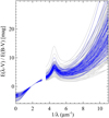 |
Fig. 1 Diversity of reddening curves by Valencic et al. (2004), Fitzpatrick & Massa (2007), and Gordon et al. (2009) of the input sample (Sect. 2, grey) and the high-quality Milky Way sample (blue, Table 4). |
4 Stellar classification
Accurate stellar classification is of utmost importance for deriving the reddening. A SIMBAD search of the MK classification in our sample (Sect. 2) shows a large spread in the SpT and the LC. In order to reduce systematics we therefore re-classified the SpT of our stars in the MK system using UVES spectra that were fitted to standard stars. For the standard star spectra we used the library “libr18” by Gray & Corbally (2014). The library includes spectra at wavelengths between 380 and 462 nm. The reduction and analysis of the UVES spectra are explained in Paper I (Siebenmorgen et al. 2020) and were complemented with spectra available in the ESO Science Archive Facility under ESO programme IDs listed in the acknowledgements. The UVES spectra are at a resolving power of λ/Δλ ~ 75 000 and high signal-to-noise (≥200). The different settings of the UVES spectra were rectified, merged, shifted in wavelength to match the 410.2 nm feature, and smoothed by a Gaussian kernel to equal the spectral resolution of the spectra in the library. SpT and LC were determined by the best-fitting element of the library to the spectrum of the target star. The best fit was identified using a minimum χ2 condition.
The precision in the classification of O-type stars was estimated by comparing the Walborn & Fitzpatrick (1990) standards to the SpT derived in the Galactic O-star survey by Sota et al. (2014). There are 34 O-stars common to both catalogues. For 32 stars the SpT agrees to better than one subclass and for two stars the SpT differs by more than that. These are HD 093129 and HD 303308; both are O3 standards by Walborn & Fitzpatrick (1990) whereas Sota et al. (2014) classifies them in agreement to our fitting procedure as O5 and O4.5, respectively.
Additionally, our SpT and LC estimates were compared with classifications of early-type standards by Walborn & Fitzpatrick (1990). These authors provide 38 O-type and 37 B-type standard stars with different LCs. The Gray & Corbally (2014) library includes 24 spectra for stars between O4 and O9 and 37 spectra for stars between B0 and B9. Our SpT agrees to better than one subclass for 36 stars. A larger spread is only found for two stars; HD 037043 is classified as an O9V and HD 163758 as an O6.5Ia standard by Walborn & Fitzpatrick (1990); in agreement with Sota et al. (2014) we assign SpT of O7V and O5Ib, respectively. Most of the 37 B stars are earlier than B3 with only one B5 and one B8 star. Our SpT estimates match to within better than one subclass for 35 of these stars. Only HD 51309 and HD 53138, both classified as B3Iab Walborn & Fitzpatrick (1990), yield B5Iab in our fitting procedure.
The goodness of the Gray & Corbally (2014) best-fit to the 75 OB standard star spectra by Walborn & Fitzpatrick (1990) is at minimum χ2 = 0.5 ± 0.6 < 1.45 and the ratio of both spectra varies by 2.4 ± 0.4 < 3.7 (%). The SpT estimates of the stars agree to within ΔSpT = 0.6 ± 0.3. Gray & Corbally (2014) distinguish luminosity classes I, III, and V. The LC determination of our procedure agrees with Walborn & Fitzpatrick (1990) to ΔLC = 0.5 ± 0.8. The accuracy of the classification on the MK system by our fitting procedure is the same as reached by Gray & Corbally (2014). These authors report a precision comparable to human classifiers of ΔSpT = 0.6 of a spectral subclass and ΔLC = 0.5 of a luminosity class, respectively. Liu et al. (2019) classified stellar spectra of the LAMOST survey using Gray & Corbally (2014) and confirm the quoted accuracy. A similar precision in stellar classification is also reached by Kyritsis et al. (2022), again indicating the accuracy of our classification is on a par with other works in the literature.
The SpT procedure was also applied to the unreddened comparison stars by Cardelli et al. (1989) and Gordon et al. (2009). The ELODIE1 and ESO archives2 were inspected for available data from high-resolution spectrographs ELODIE (Moultaka et al. 2004), ESPRESSO (Pepe et al. 2021), FEROS (Kaufer et al. 1999), HARPS (Mayor et al. 2003), X-shooter (Vernet et al. 2011), and UVES. High-resolution spectra of 21 standards were found and the various SpT estimates agree to previous estimates within one subclass (Table 1).
Spectral-types of unreddened comparison stars.
5 Scrutinizing reddening curves
Reddening curves offer the possibility of deriving fundamental characteristics of dust such as particle sizes and abundances. Systematic issues that affect reddening curves must be minimized for dust modelling work. To this aim, the trustworthiness of the reddening curves towards the 111 stars presented in Sect. 2 have been inspected to establish a high-quality reddening curve sample with predominantly single-cloud sightlines.
According to Eq. (5) reddening curves have a similar shape making it extremely difficult to exclude less good cases by simple inspection (Fig. 1). Even if there exist comparable results for the same star, there might still be errors whenever the conditions for the derivation of the reddening are not fulfilled. The quality of the reddening curve depends critically on the precision of the SpT and LC estimates, the photometric and spectral stability of the reddened and unreddened star, the de-reddening of the comparison star, and the photospheric model when applied. In general, reddening curves are derived assuming single stellar systems.
In the following subsections, we discuss the systematic effects that affect the reddening curves of our sample. A comparison of spectral-type between the reddened and the unreddened star is given in Table 2. Uncertain cases and those that are not qualified for detailed dust modelling are rejected and listed in Table 3, while the sample of high-quality reddening curves are given in Table 4.
5.1 Parametrization of reddening curves
Reddening curves in the UV range between 3.3 µm−1 ≲ λ−1 ≲ 11 µm−1 are represented by a spline fit, a Drude profile for the 2175 Å extinction bump, and a polynomial for the UV rise
 (5)
(5)
where x = λ−1. The Drude profile is given by
 (6)
(6)
with damping constant y and central wavelength  . The nonlinear increase of the reddening in the far UV is described by F(x). Gordon et al. (2009) and Valencic et al. (2004) applied a form that is given by Fitzpatrick & Massa (1990)
 (7)
(7)
while Fitzpatrick & Massa (2007) used
 (8)
(8)
At longer wavelengths F(x) = 0. Following Gordon et al. (2009), we reduce c4 by 7.5% when data from the IUE alone were used to estimate the reddening curve, and extrapolate the reddening to x = 11 µm−1 when necessary. Reddening in spectral regions close to wind lines at 6.5 and 7.1 µm−1 and Ly-α at 8 µm−1 ≤ x ≤ 8.45 µm−1, or with apparent instrumental noise at x ≲ 3.6 µm−1 is ignored.
Relations between the reddening curve parameters ci and RV (Eq. (5)) and the dust model parameters are given in Table 5 by Siebenmorgen et al. (2018b). For example, an uncertainty of 10% in c1 implies an uncertainty of 5% in the abundance ratio of the large silicate to carbon particles; a 10% error in RV translates into a variation of the exponent q of the dust size power-law distribution of 10%. Eventually, a variation of 10% in c4 results in an uncertainty in the abundance ratio of very small to large grains of ≳25%.
5.2 Composite FUSE and IUE spectra
Reddening curves derived from a composite spectrum that includes the programme star and other bright objects are invalid. Reddening curves of our sample are flagged when there are multiple objects in the IUE (separation ≤ 10″) or in the FUSE aperture (separation ≤ 15″) that contribute by more than 10% to the flux of the programme star (ΔV ≲ 2.5 mag). The HIPPARCOS (ASCC-2.5; Kharchenko & Roeser 2009) and SIMBAD databases were also used to detect potential contaminating objects. For 12 stars the label M is assigned in Table 3 indicating that the observed spectrum is a composite of multiple bright objects in the IUE aperture. No companions were found in the FUSE aperture.
5.3 Multiple star systems
The multiplicity of stellar systems is typically investigated through imaging and interferometry (Sana et al. 2014) and/or spectroscopy (Chini et al. 2012). The latter method is biased towards finding close companions down to a few AU separation by providing a measure of time variable radial velocities. Differences in the line profiles are still visible in inclined systems for which the brightness difference between primary and companion may become marginal. Such a high-resolution radial velocity survey with spectra taken at multiple epochs (2–12) of about 800 OB stars is presented by Chini et al. (2012). Companions in that survey are detected down to a brightness difference of ΔV ~ 2 mag. This translates to detectable companions of an O5 star range between O5 and B2, and those of a B9 star from B9 to A7. The results of the surveys listed above indicate that nearly 100% of O-type stars have one or more companions within 1 mas to 8″ separation and at a contrast down to ΔH = 8 mag (Sana et al. 2014), falling to 80% for early-B and to 20% for late B-types (Chini et al. 2012). The HIPPARCOS Tycho photometric catalogue (Kharchenko & Roeser 2009) provides various labels indicating the duplicity or variability status of the stars. Unfortunately, there are no striking features in the reddening curves noticeable when inspecting sub-samples with variability and binary flag set or unset.
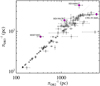 |
Fig. 2 Inverse parallax (pc) of Gaia data releases DR3, |


5.4 Gaia
The Gaia space observatory launched by the European Space Agency (ESA) in 2013 measures positions, parallaxes, motions, and photometry of stars with unprecedented precision (Gaia Collaboration 2016). The Gaia data release 2, DR2 (Gaia Collaboration 2018) was based on observations made between July 2014 and May 2016 and was followed by data release 3, DR3 (Vallenari et al. 2022) which includes observations until May 2017.
Stars that have inconsistent Gaia parallaxes πDR2 versus πDR3 are suspicious. Their parallax measurements at higher than 3σ confidence remain unconfirmed either due to instrumental artefacts, which we doubt, bright companions or stellar activity. In our sample, there are 102 stars with parallax measurements in DR2 at a typical signal-to-noise ratio of 13; in DR3 there are 106 of our stars with a typical signal-to-noise ratio of 25. From these stars, 95 have a ratio πDR2/πDR3 higher than 3σ confidence with a mean ratio of 0.94 ± 0.16. The 6% deviation from unity is driven by unsecured DR2 measurements at large distances. By considering a sub-sample with  ≲ 2 kpc there are 72 stars with a mean ratio of πDR2/πDR3 ~ 0.98 ± 0.14 which is consistent with being unity. Four stars are identified by 3σ clipping as outliers and are indicated with the flag π in Table 3. The inverse parallax (pc) of
  versus
  is shown with outliers marked in magenta in Fig. 2. We note the deviation from the identity curve at
  ≳ 2 kpc.
The photometric stability of the stars of our sample was verified by comparing both Gaia data releases. In Fig. 3 the differences in G band (330–1050 um) photometry between DR3 and DR2, ΔG = GDR3 – GDR2, is shown for our sample of 111 stars. In that sample, the mean and 1σ scatter of ΔG = 14 + 11 mmag. Nine stars show variability in the photometry with ΔG outside of the range 14 ± 33 mmag. They are marked in Fig. 3 in magenta outside the ± 3σ curves shown as dashed lines. Their reddening curves are classified as uncertain. Six of these sightlines were not yet rejected and they are labelled ΔG in Table 3.
We note that seven stars from our sample would be rejected due to colour variability in B – G, whereas stars outside of the range (B – G)DR3 – (B – G)DR2 of 31 ± 66 mmag would be excluded using 3σ clipping. These stars were already rejected using the previous criteria.
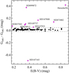 |
Fig. 3 Differences in Gaia G band photometry between data release DR3 and DR2, GDR3 – GDR2, as a function of reddening E(B – V). Stars labelled in magenta outside the dashed lines are rejected. |
5.5 Photometric variability
Stellar variability will impact the results for reddening. Early-type stars may vary due to multiplicity or due to winds. About 50% of OB stars reveal extra-photospheric infrared excess emission that is likely caused by winds (Siebenmorgen et al. 2018a; Deng et al. 2022), and strikingly, as discussed in Sect. 5.3, the great majority of O and early-type B stars form close binary systems.
The reddening curves that we obtained from the literature made use of the Johnson UBV system (Hiltner & Johnson 1956; Nicolet 1978). Ground-based (GB) photometry of our sample is given by Valencic et al. (2004) and refers to observations between 1950 and 2000. Stellar photometry from the HIPPARCOS satellite between 1989–1993 is also available. Kharchenko & Roeser (2009) merged HIPPARCOS, Tycho, PPM, and CMC 11 observations of 2.5 million stars and transformed V and B magnitudes to the Johnson system. This resulted in a colour-dependent correction of 20–40 mmag, and a typical error below 10 mmag of the ASCC-2.5 catalogue (Kharchenko & Roeser 2009).
The photometric stability of the stars was verified by comparing ground-based VGB Valencic et al. (2004) and HIPPARCOS VHip Kharchenko & Roeser (2009) photometry (Fig. 4). There are 73 stars for which photometry in both catalogues is available and which are not rejected by the previous confidence criteria (Sects. 5.2–5.4). In that sample the mean and 1σ scatter of ΔV = VGB – VHip = 5 ± 31 mmag. The small offset is within the photometric error. Seven stars are identified by 3σ clipping as outliers showing significant variability in the V band. Their reddening curves are classified as uncertain and labelled ΔV in Table 3. These stars are marked in magenta in Fig. 4 and are outside the ±3σ variation shown as dashed lines. HD 037023 was identified as a composite star in Sect. 5.2 and fails with ΔV = 1.6 mag. The photometric variable star HD 091983 was used by Gordon et al. (2009) to derive the reddening curves towards HD 122879 (Table 1) and HD 168941.
The same procedure of outlier rejection was repeated by comparing the B band photometry and the (B – V) colour provided from the ground by Valencic et al. (2004) and by HIPPARCOS (Kharchenko & Roeser 2009). The mean and 1σ scatter in the colours is ΔBV = (B – V)GB – (B – V)HiP = −28 ± 28 mmag. The two stars HD 147701 and HD 169454 are identified by 3σ clipping as outliers. Their reddening curves are classified as uncertain and labelled ΔBV in Table 3. No additional stars were rejected due to photometric variability in the B band.
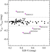 |
Fig. 4 Differences in V band photometry between ground-based (Valencic et al. 2004) and HIPPARCOS (Kharchenko & Roeser 2009) VGB – VHip as a function of reddening E(B – V). Stars labelled in magenta outside the dashed lines are rejected. |
5.6 Unfeasible stellar classification
O- and B-type stars are often fast rotators; the peak in the rotational velocity probability distribution for B-type stars is around 300 km s−1 (Dufton et al. 2019). As a consequence their SpT and LC determination is highly uncertain because: (1) most useful diagnostic lines such as Mg II or He I are blended and (2) unless the spectra have a very high signal-to-noise ratio, many stellar absorption lines merge into the continuum. Several of the stars have also a bright companion making the stellar classifcation unfeasible. For nine stars the stellar classification procedure of Sect. 4 is uncertain at χ1 > 2. These sightlines are rejected for the high-quality reddening curve determination with label χ2 in Table 3.
5.7 Inaccurate stellar classification
A SpT and LC miss-match of the target or comparison star can give a large variation in E(B – V), in the infrared extinction, differences in position and width of the extinction bump, and in the far UV rise of the reddening curve. As shown by Massa et al. (1983); Massa & Fitzpatrick (1986); Cardelli et al. (1992), photometric and systematic errors of the extinction curves scale as 1/E(B – V). A miss-classification in the LC or SpT of more than one subclass in either of the reddend or the unreddened star may introduce large (~20%) systematic errors in E(B – V) and a significant difference in the far UV rise (Cardelli et al. 1992). They also show that such a change in the far UV rise expressed in parameter c4 (Eq. (5)) may vary by a factor ~1.5. Whenever the comparison star is hotter than the reddened star the far UV rise will be overestimated. In the UV, the IUE and FUSE spectrographs were used to estimate SpT and LC. Besides the low resolving power of these UV spectrographs, there are major diagnostic lines in the optical but not in the UV. Smith-Neubig & Bruhweiler (1997) show that the UV spectral diagnostics indicate often earlier SpT than obtained from optical spectra. They considered uncertainties of one LC and one SpT, which increases to up to two sub-types for mid/late B stars because of fewer spectral diagnostics in that range.
Gordon et al. (2009) list the SpT of the reddened and comparison stars. Valencic et al. (2004) apply comparison stars selected from Cardelli et al. (1992), who provide those for types earlier than B3. For later stars, the choice of the comparison star was not detailed; same holds for stars earlier than O7. We note that the stellar atmosphere model-based method, as used by Fitzpatrick & Massa (2007), does not need to apply a comparison star. For some stars we find differences in the SpT and LC of more than one subclass when derived from observations in the UV by Valencic et al. (2004), Fitzpatrick & Massa (2007), and Gordon et al. (2009) and in the optical (Sect. 4). This introduces systematic errors in the reddening curves as mentioned above. This affects fifteen curves by Valencic et al. (2004), two by Gordon et al. (2009), and six by Fitzpatrick & Massa (2007). For the latter there is an extra difficulty that the temperature of the Lanz & Hubeny (2007) model atmospheres needs to be related to the MK system by means of a stellar temperature scale (Theodossiou & Danezis 1991). In that scheme we add an extra uncertainty of 1,000 K in favour of non-rejection.
In 40 out of 54 cases, the SpT of the reddened and the comparison stars agree within 1.5 subclasses. These stars are indicated below the line in Table 2 and are kept in the high-quality sample, whereas the cases above that line show larger deviations. Their reddening curves are considerered to be of lower quality. For example, the SpT of HD 093843 is uncertain; we find O4 Ib, Sota et al. (2014) O5 III, and Valencic et al. (2004) O6 III. For deriving the reddening curve Valencic et al. (2004) used an O7 V comparison star, which deviates by more than two types; therefore, we reject the reddening. HD 046660 whose SpT is also uncertain, when using the fitting procedure (Sect. 4), a similar χ2 minimum is found for either B0 III or O7 V. We adopt the latter type as the star displays He II. It has been classified as O9 V by Siebenmorgen et al. (2020) implying a temperature ≳30,000 K, in agreement with 31067 K derived Fitzpatrick et al. (2019). However, Fitzpatrick & Massa (2007) derived the reddening with a best fitting model atmosphere at 26,138 K, hence later than B1 (Theodossiou & Danezis 1991; Pecaut & Mamajek 2013). Additionally, Valencic et al. (2004) derived the reddening with a B1.5 V comparison star. Due to the discrepancy between these results and our derived SpT, we also reject this reddening curve. As detailed in Table 2, the reddening curve of HD 168076 (O4 III/O5 V) was derived by Valencic et al. (2004) using an O5 V type star, while Gordon et al. (2009) used HD 091824 (O7 V) and is therefore removed. For HD 167771 the reddening curve by Valencic et al. (2004) was derived with a comparison star that differs by two subclasses and is removed, while the Gordon et al. (2009) derived curve with a smaller SpT difference is included (Table 2). The reddening curve towards HD 108927 (B5 V) was derived by Valencic et al. (2004) using a B3 V comparison star. Reddening curves derived with comparison stars with unconfirmed SpT in Simbad are kept. For example, Gordon et al. (2009) used as comparison stars HD 051013 (B3V?) for deriving the reddening of HD 027778 (B3 V) and HD 062542 (B5 V). Both reddening curves show excellent agreement with those derived by Fitzpatrick et al. (2019), respectively. Further comments on individual stars are given in Appendix A. In total, 15 sightlines have uncertain reddening curves because of a SpT mismatch (Table 2). They are flagged in Table 3 by attaching the SpT and LC to that star.
Comparison of spectral-type between the reddened and the unreddened star.
5.8 Comparison of reddening derived from the IUE and Ground-based observations
After applying the confidence criteria, we discovered that some of the remaining reddening curves display a jump when going from the longest wavelength of the IUE spacecraft, that is not contaminated by instrumental features at 0.28 µm, to the shortest wavelength accessible from the ground, the U band. The reddening between 0.28 µm and the U band for these 96 curves has a mean and 1σ scatter of E(0.28µm–U)/E(B – V) = 1.3 ± 0.3 mag and are shown in Fig. 5. Peculiar reddening curves that show an offset in E(0.28µm – U)/E(B – V) were identified by means of 3σ clipping. These include eight reddening curves which are derived by Valencic et al. (2004). Two of these, HD 108927 and HD 122879, were rejected above. For HD 079286, HD 089137, and HD 149038 no other reddening curve is available. For the remaining three sightlines – HD 091824, HD 156247, and HD 180968 – only the reddening curves derived by Valencic et al. (2004) show this striking jump whereas this feature is not present in the reddening curves derived by Fitzpatrick & Massa (2007) for the same stars (Fig. 7). These six reddening curves are marked as peculiar in Table 4.
6 The high-quality sample of reddening curves in the Milky Way
6.1 The sample
Our high-quality sample contains only reddening curves that respect the following six confidence criteria derived in Sect. 5: (a) the IUE spectra include only a single star that dominates the observed spectrum. (b) The Gaia parallaxes πDR3 and πDR2 are consistent within their 3σ error estimates. (c) The Gaia photometric variability between DR3 and DR2 is within −19 ≲ ΔG ≲ 47 (mmag). (d) The variability of the star observed from the ground and by HIPPARCOS in the V band is within −100 ≲ ΔV ≲ 88 (mmag) and in the B–V colour within −55 ≲ ΔBV ≲ 112 (mmag), respectively. (e) SpT and LC are derived as in Sect. 4 at high confidence (χ2 < 2). (f) The stellar classification of programme and comparison star agrees within one subtype.
With these confidence criteria, the high-quality sample is given in Table 4. It comprises 80 reddening curves for 53 sight-lines of which 35 are the rare cases of single-cloud dominated sightlines. Six reddening curves show a peculiar jump between 0.28 µm and the U band of E(0.28µm–U)/E(B – V) > 2.2 mag. We give preference to reddening curves by Gordon et al. (2009) as they include besides IUE also FUSE data. We also prefer reddening curves by Fitzpatrick & Massa (2007) over Valencic et al. (2004) because comparison star observations that were used in the latter work are not needed in the former derivation procedure. Our choice of the reference reddening curve EReſ for each sightline is given in Col. 3; when available, other accepted reddening curves Ei with i ∈ {FM07, V04} are listed in Col. 4. None of the stars of Table 4 is associated with reflection nebulosity within 5″ (Magakian 2003) as otherwise, the curves would not represent the reddening in the translucient cloud.
All reddening curves of both the high-quality sample (Table 4) and those of the stars with uncertainties in the reddening curve are shown in Figs. 6 and 7, respectively. A nearly perfect match for stars with accepted curves by Gordon et al. (2009), Fitzpatrick & Massa (2007), and Fitzpatrick et al. (2019) are visible in Fig. 6 and for about half of the stars with high-quality reddening curves by Fitzpatrick & Massa (2007) and Valencic et al. (2004) in Fig. 7. We note that the consistency between various reddening curves of a star cannot be taken as full proof of the correctness of the derivation. In the far UV a steeper rise in the reddening is present for six curves derived by Valencic et al. (2004) and for three stars by Fitzpatrick & Massa (2007) when compared to any other of the available reddening curves for these stars. In the near IR differences in the reddening between Valencic et al. (2004) and Fitzpatrick & Massa (2007) are visible for three sightlines (Fig. 7).
Rejected sightlines (58) with uncertain reddening curves.
High-quality Milky Way reddening curve sample.
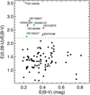 |
Fig. 5 Reddening between 0.28 µm and the U band as a function of E(B – V). The reddening curves towards the stars above the dashed line were derived by Valencic et al. (2004). They are marked in green when included in the high-quality sample (Table 4) and in red when rejected. |
6.2 Intrinsic errors in the high-quality sample
The intrinsic error of the reddening curves in the high-quality sample (Sect. 6.1) was estimated by measuring the variance between individual reddening curves towards the same star. For each star of Table 4, which is not flaged as peculiar, the ratio  of the two reddening curves was computed, where the reference for the reddening curve
  is given in Col. 3 and the reference for the reddening curve Ei with i ∈ {FM07, V04} in Col. 4 of Table 4. For example, for HD 027778 the ratio of the reddening curves
  were determined, for HD 030470 there exists no such ratio, and for HD 037903 there are even two ratios available
  and
and  . In total there are 27 (Ei/ERef) ratios of reddening curves that all pass the confidence criteria of Sect. 6.1.
The mean and 1σ error of these (Ei/EReſ) ratios are computed by omitting data at 1/λ ≳ 7.5 µm−1 when not observed by FUSE. In the V band, to which the curves are normalized, the scatter of these ratios is σ(Ei/EReſ) = 0 by definition and remains naturally small for wavelengths close to it. In the IUE range σ(Ei/ERef) ~ 10% and grows to ~15% in the far UV at x ~ 11 µm−1. Similarly σ(Ei/ERef) ≲ 7% for λ ~ 1 µm and increases to 11% at longer wavelengths. The typical error in the high-quality sample when averaged over wavelengths is σ(Ei/ERef) ~ 9% and stays below 16%. Repeating the same exercise for the 58 stars with uncertain reddening curves gives 23 such ratios and shows a larger scatter of σ(Ei/ERef) ~ 15%. The ratios of uncertain reddening curves of the same star varies by up to 39%, which is about a factor of two larger spread than for the high-quality sample.
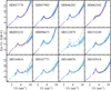 |
Fig. 6 Comparison of reddening curves derived for the same sightline. The symbols represent the reddening data from Gordon et al. (2009) shown as blue dots and by Fitzpatrick et al. (2019) in salmon, respectively. Reddening curves derived from UV spline fits (Eq. (5)) and interpolated in UBVJHK, –RV are taken from Gordon et al. (2009), shown as blue, by Fitzpatrick & Massa (2007) in red, and by Valencic et al. (2004) by green lines. Non peculiar stars of the high-quality sample listed in Table 4 are shown as full lines with the others as dashed lines. |
6.3 Uncertainties in RV
The shape of the extinction curves depends on the total-to-selective extinction RV (Cardelli et al. 1989; Zagury 2020). This parameter is estimated by extrapolating a derived reddening, for example, in the near or mid infrared, to infinite wavelengths; thus RV is not an observable. It successfully describes averaged properties with clear deviations in the reddening for specific sightlines (Gordon et al. 2023). The systematic uncertainties of RV = −E(∞) (Eq. (3)) are hence of interest. The differences ΔRV = Eref(∞) – Ei(∞) of the available estimates of RV for the same star are computed. They provide an estimate of the systematic errors and are shown in Fig. 8 as histograms for the sample of uncertain and confident reddening curves. The references to the reddening curves Eref and Ei are listed for the high-quality sample in Cols. 3 and 4 of Table 4. For the unsecure sample we use – whenever available – the estimate of Eref(∞) by Gordon et al. (2009) and otherwise Fitzpatrick & Massa (2007). Three stars HD 104705, HD 164073 and HD 147933 deviate with ||ΔRV|| > 1.3 and are therefore omitted. For example, HD 164073 has RV = 2.96 (Valencic et al. 2004) or RV = 5.18 (Fitzpatrick & Massa 2007). The distributions in ΔRV appear similar in both samples and are flatter than Gaussian, which indicates that systematic errors dominate. The high-quality sample has a peak-to-peak scatter, mean, and 1σ error of −0.33 ≲ ΔRV = 0.09 ± 0.21 ≲ 0.67. The reference reddening curves of the high-quality sample vary between 2.01 ≲ RV = 3.08 ± 0.44 ≲ 4.34 (Sect. 6.4). We find that the derivation of RV for the same star by the various authors agrees to better than σ(ΔRV)/mean(RV) ~ 7%.
6.4 Reddening in the Milky Way
Galactic extinction studies derive the typical wavelength dependence of interstellar reddening. Such curves are commonly used, in particular in extra-galactic research, as the standard for dered-dening the observed flux of objects for which there is no specific knowledge about the dust. Large variations from cloud-to-cloud of the grain characteristics and the physical parameters of the dust are reported by Siebenmorgen et al. (2018b). Although aver- aging a sufficiently large number of clouds and sightlines leads to similar mean parameters, they likely do not reflect the true nature of the dust. The degree to which mean Galactic extinction curves can be taken as typical shall always be put in question.
The shape of the average Galactic extinction for a sample of 243 stars with 2.4 ≤ RV ≤ 3.6 at 1/λ ≤ 8.6 µm−1 has been presented by Fitzpatrick & Massa (2007). Their mean curve has RV = 3.1 as derived earlier by Fitzpatrick & Massa (1990) and Valencic et al. (2004) and in recent studies (Fitzpatrick et al. 2019); Wang & Chen (2019) find a similar value of RV = 3.16. Here we compute average Milky Way reddening curves using the high-quality sample (Table 4, Col. 3). As in the previous sections a 3σ rejection criterium is applied, so that stars have AV ≲ 2.4 and RV ≲ 4.4. HD 093222 and HD 168076 violate this criterium and are not included in the analysis. We distinguish sightlines of translucent clouds at 1 < τV ≲ 2.2 and single-cloud sightlines of the diffuse ISM at τV ≲ 1. The average curve of the 33 translucent clouds in our sample has a peak-to-peak scatter, mean, and 1cc error of 2.7 ≲ RV = 3.3 ± 0.4 ≲ 4.1 at median of RV = 3.16. That of the 15 single-cloud diffuse ISM sightlines has 2.3 ≲ RV = 3.0 ± 0.3 ≲ 3.6 at median of RV = 3.1, respectively. These curves3 are shown in Fig. 9 with the average Galactic reddening by Fitzpatrick & Massa (2007) and Fitzpatrick et al. (2019). Driven by the same RV of these curves a nearly perfect match from optical to longer wavelengths is found; for translu- cent clouds this incldues the IUE range and for the diffuse ISM the reddening is smaller at λ < 0.2µm. Noticeable is the large diversity of the reddening curves (Fig. 1) and agreement of the various mean Milky Way reddening curvesl within σ (RV) = 0.4.
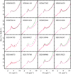 |
Fig. 7 Comparison of reddening curves derived for the same sightline. Notation as in Fig. 6: Valencic et al. (2004) in green, Fitzpatrick & Massa (2007) in red, and Fitzpatrick et al. (2019) in salmon. |
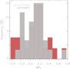 |
Fig. 8 Systematic differences in estimates of the total-to-selective extinction. The histograms show ΔRV = Eref(∞) - Ei(∞) of individual stars in the sample with uncertain (red) and confident reddening curves (grey). |
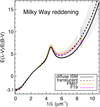 |
Fig. 9 Milky Way reddening derived from the high-quality sample (Table 4) for translucent clouds (dashed with 1σ error bars) and for single-cloud sightlines of the diffuse ISM. The average Galactic redden- ing derived by Fitzpatrick & Massa (2007) and Fitzpatrick et al. (2019) are shown for comparison. |
7 Summary
Individual clouds in the ISM can be drastically different from each other. Therefore, the framework of single-cloud sightlines was introduced as they provide an unambiguous view of phys- ical relations between dust properties and observables such as extinction and polarization (Siebenmorgen et al. 2018b, 2020). Reddening curves allow to derive fundamental characteristics of dust. However, before extracting dust properties from a physical model one must ensure that the observational basis is solid and the assumptions in the derivation of the reddening are met to an acceptable level.
We discussed the current database of available reddening curves. The initial sample of 820 reddening curves towards 568 OB stars, which cover the spectral range from the near IR to the Lyman limit was merged with 186 OB stars with high- resolution UVES spectra and with polarization spectra towards 215 OB stars from the Large Interstellar Polarization survey. This yields a sample of 111 sightlines for which the redden- ing curves were scrutinized against systematic errors by the following means:
Whenever IUE/FUSE spectra were identified as a com- posite of multiple bright sources the corresponding reddening curves were rejected. Stars with assigned binary information did not provide a direct link or a striking feature in the appearance of the reddening curves for qualifying a rejection.
The stellar classification of the stars was derived at high confidence. Objects whose SpT do not match within one subtype the comparison star were removed from the sample.
Stars with detected variability between 1950 and 2017 from ground-based and HIPPARCOS V band photometry and B – V colurs of about 0.1 mag were excluded. The same holds for Gaia G band photometric variations of more than 47 mmag.
Reddening curves of stars showing inconsistencies in the Gaia parallaxes between DR2 and DR3 were declared as spurious.
The reddening curves with different estimates of RV of the same star exceeding 50% were also rejected.
In total, we find 50 stars with one or more not perculiar red- dening curves passing the rejection criteria of which 35 are the rare cases of single-cloud sightlines. This provides the highest-quality Milky Way reddening curve sample available today. The average Milky Way reddening curve is determined for translucent clouds and the diffuse ISM to be RV = 3.1 ± 0.4, confirming earlier estimates. The high-quality reddening curve sample together with polarization properties will be subject to dust modelling in a future paper in this series of the Dark Dust project.
Acknowledgements
J.K. acknowledges the financial support of the Polish National Science Centre, Poland (2017/25/B/ST9/01524) for the period 2018–2023. This research has made use of the services of the ESO Science Archive Facility and the SIMBAD database operated at CDS, Strasbourg, France (Wanger et al. 2000) and partially based on observations collected at the European Southern Observatory under ESO programmes Observations collected at the European Southern Observatory are based under ESO programmes: 060.A-9036(A), 067.C-0281(A), 071.C-0367(A), 072.D-0196(A), 073.C-0337(A), 073.C-0337(AX073.D-0609(AX074.D-0300(AX075.D-0061(A),075.D-0369(AX 075.D-0369(AX076.C-0164(AX076.C-0431(A),076.C-0431(BX079.D-0564(AX 081.C-0475(A),081.D-2008(A),082.C-0566(A),083.D-0589(A),083.D-0589(A), 086.D-0997(B),091.D-0221(A),092.C-0019(A), 102.C-0040(B), 102.C-0699(A), 187.D-0917(A), 194.C-0833(A), 194.C-0833(B), 194.C-0833(D),194.C-0833(E), 194.C-0833(F),194.C-0833(H),0102.C-0040(B),072.A-0100(A),072.B-0123(D), 072.B-0218(A),072.C-0488(E),076.B-0055(A),077.C-0547(A),078.D-0245(C), 079.A-9008(A),079.C-0170(A),083.A-0733(A),088.A-9003(A),089.D-0975(A), 091.C-0713(A),091.D-0221(A),092.C-0218(A),096.D-0008(A),097.D-0150(A), 106.20WN.001,1102.A-0852(C),165.N-0276(A),194.C-0833(A),194.C-0833(B), 194.C-0833(C), 266.D-5655(A), 65.H-0375(A), 65.N-0378(A), 65.N-0577(B), 70.D-0191(A).
Appendix A Comments on indiviudal stars
Reddening curves with a miss-match of more than one type between our estimates (Sect. 4) and the SpT used in the deriva- tion are rejected by the following reason:
HD 054306: we classify it as B3V whereas Fitzpatrick & Massa (2007) finds it at 22,409 K so earlier than B1.5 I and Valencic et al. (2004) used a B1 V comparison star (HD 031726).
HD 072648: we classify it as B5 Ib whereas Fitzpatrick & Massa (2007) finds it at 21,035 K so earlier than B1.5 I and Valencic et al. (2004) used a B1.5 III comparison star.
HD 091983: we classify this photometric variable star (Fig. 4) as O9 V, Sota et al. (2014) as O9 IV, and Cardelli et al. (1992) finds it as O9.5 Ib.
HD 096675: we classify it as B7 V, Gordon et al. (2009) as B6 IV and Valencic et al. (2004) used a B5 V comparison star.
HD 103779: we classify it as B2 Ib whereas Gordon et al. (2009) and Valencic et al. (2004) used a B0.5 Ib comparison star.
HD 134591: we classify it as B8 III whereas Valencic et al. (2004) used a B4 V comparison star.
HD 151804, HD 153919, HD 162978: we classify these stars as O 8Ia, O4 Ib, O8II and Sota et al. (2014) as O8 lab, O6 V, O8 III; whereas Valencic et al. (2004) used a O 9.5Ia comparison star.
HD 164536: we classify it, in agreement to Sota et al. (2014), as O7 V whereas Fitzpatrick & Massa (2007) finds it at 33,500 K, close to O9 V (Theodossiou & Danezis 1991).
HD 164816: we classify it as O8 V, Sota et al. (2014) as O9.5 V+B0 V binary, Valencic et al. (2004) as B0 V, and Fitz-patrick & Massa (2007) finds it at 31,427 K, close to O9.5 V (Theodossiou & Danezis 1991), while Gordon et al. (2009) used HD 097471 a B0 V comparison star.
HD 168076: we classify it as O5 V at χ2 = 0.31 and as O4 III at χ2 = 0.17 in agreement to Sota et al. (2014).
HD 185859: we classify it as B2 Ib whereas Valencic et al. (2004) used a B0.5 Ib comparison star.
HD 203532: we classify it as B5 III, Fitzpatrick & Massa (2007) finds it at 17,785 K so earlier than that (Theodossiou & Danezis 1991) and Valencic et al. (2004) used a B3 IV comparison star.
HD 315033: we classify it as B3 V whereas Fitzpatrick & Massa (2007) finds it at 25,609 K so earlier than B1.5 V and Valencic et al. (2004) used a B1.5 III comparison star.
References
- Allamandola, L. J., Tielens, A. G. G. M., & Barker, J. R. 1989, ApJS, 71, 733 [Google Scholar]
- Bagnulo, S., Cox, N. L. J., Cikota, A., et al. 2017, A&A, 608, A146 [NASA ADS] [CrossRef] [EDP Sciences] [Google Scholar]
- Binder, B. A., & Povich, M. S. 2018, ApJ, 864, 136 [CrossRef] [Google Scholar]
- Bouwman, J., Meeus, G., de Koter, A., et al. 2001, A&A, 375, 950 [NASA ADS] [CrossRef] [EDP Sciences] [Google Scholar]
- Cardelli, J. A., Clayton, G. C., & Mathis, J. S. 1989, ApJ, 345, 245 [Google Scholar]
- Cardelli, J. A., Sembach, K. R., & Mathis, J. S. 1992, AJ, 104, 1916 [NASA ADS] [CrossRef] [Google Scholar]
- Chini, R., Hoffmeister, V. H., Nasseri, A., Stahl, O., & Zinnecker, H. 2012, MNRAS, 424, 1925 [Google Scholar]
- Cutri, R. M., Skrutskie, M. F., van Dyk, S., et al. 2003, 2MASS All Sky Catalog of point sources (NASA/IPAC Infrared Science Archive) [Google Scholar]
- Dekker, H., D’Odorico, S., Kaufer, A., Delabre, B., & Kotzlowski, H. 2000, SPIE Conf. Ser., 4008, 534 [Google Scholar]
- Deng, D., Sun, Y., Wang, T., Wang, Y., & Jiang, B. 2022, ApJ, 935, 175 [NASA ADS] [CrossRef] [Google Scholar]
- Dickey, J. M., & Lockman, F. J. 1990, ARA&A, 28, 215 [Google Scholar]
- Dufton, P. L., Evans, C. J., Hunter, I., Lennon, D. J., & Schneider, F. R. N. 2019, A&A, 626, A50 [NASA ADS] [CrossRef] [EDP Sciences] [Google Scholar]
- Fitzpatrick, E. L., & Massa, D. 1990, ApJS, 72, 163 [NASA ADS] [CrossRef] [Google Scholar]
- Fitzpatrick, E. L., & Massa, D. 2007, ApJ, 663, 320 [Google Scholar]
- Fitzpatrick, E. L., Massa, D., Gordon, K. D., Bohlin, R., & Clayton, G. C. 2019, ApJ, 886, 108 [Google Scholar]
- Gaia Collaboration (Prusti, T., et al.) 2016, A&A, 595, A1 [NASA ADS] [CrossRef] [EDP Sciences] [Google Scholar]
- Gaia Collaboration (Brown, A. G. A., et al.) 2018, A&A, 616, A1 [NASA ADS] [CrossRef] [EDP Sciences] [Google Scholar]
- Gordon, K. D., Cartledge, S., & Clayton, G. C. 2009, ApJ, 705, 1320 [NASA ADS] [CrossRef] [Google Scholar]
- Gordon, K. D., Clayton, G. C., Decleir, M., et al. 2023, ApJ, 950, 86 [CrossRef] [Google Scholar]
- Gray, R. O., & Corbally, C. J. 2014, AJ, 147, 80 [CrossRef] [Google Scholar]
- Hartmann, J. 1904, ApJ, 19, 268 [Google Scholar]
- Heger, M. L. 1922, Lick Observ. Bull., 10, 141 [NASA ADS] [CrossRef] [Google Scholar]
- Hensley, B. S., & Draine, B. T. 2021, ApJ, 906, 73 [NASA ADS] [CrossRef] [Google Scholar]
- Hiltner, W. A., & Johnson, H. L. 1956, ApJ, 124, 367 [NASA ADS] [CrossRef] [Google Scholar]
- Kaufer, A., Stahl, O., Tubbesing, S., et al. 1999, The Messenger, 95, 8 [Google Scholar]
- Kharchenko, N. V., & Roeser, S. 2009, VizieR Online Data Catalog: I/280B [Google Scholar]
- Krügel, E. 2008, An introduction to the Physics of Interstellar Dust (Taylor & Francis) [Google Scholar]
- Kyritsis, E., Maravelias, G., Zezas, A., et al. 2022, A&A, 657, A62 [NASA ADS] [CrossRef] [EDP Sciences] [Google Scholar]
- Lanz, T., & Hubeny, I. 2007, ApJS, 169, 83 [CrossRef] [Google Scholar]
- Li, A., & Draine, B. T. 2001, ApJ, 554, 778 [Google Scholar]
- Liu, Z., Cui, W., Liu, C., et al. 2019, ApJS, 241, 32 [CrossRef] [Google Scholar]
- Magakian, T. Y. 2003, A&A, 399, 141 [NASA ADS] [CrossRef] [EDP Sciences] [Google Scholar]
- Massa, D., & Fitzpatrick, E. L. 1986, ApJS, 60, 305 [NASA ADS] [CrossRef] [Google Scholar]
- Massa, D., Savage, B. D., & Fitzpatrick, E. L. 1983, ApJ, 266, 662 [NASA ADS] [CrossRef] [Google Scholar]
- Mathis, J. S., & Wallenhorst, S. G. 1981, ApJ, 244, 483 [NASA ADS] [CrossRef] [Google Scholar]
- Mayor, M., Pepe, F., Queloz, D., et al. 2003, The Messenger, 114, 20 [NASA ADS] [Google Scholar]
- McKee, C. F., & Ostriker, J. P. 1977, ApJ, 218, 148 [NASA ADS] [CrossRef] [Google Scholar]
- Mermilliod, J. C., Mermilliod, M., & Hauck, B. 1997, A&AS, 124, 349 [NASA ADS] [CrossRef] [EDP Sciences] [Google Scholar]
- Meyer, D. M., & Blades, J. C. 1996, ApJ, 464, L179 [Google Scholar]
- Moultaka, J., Ilovaisky, S. A., Prugniel, P., & Soubiran, C. 2004, PASP, 116, 693 [NASA ADS] [CrossRef] [Google Scholar]
- Nicolet, B. 1978, A&AS, 34, 1 [NASA ADS] [Google Scholar]
- Pecaut, M. J., & Mamajek, E. E. 2013, ApJS, 208, 9 [Google Scholar]
- Pepe, F., Cristiani, S., Rebolo, R., et al. 2021, A&A, 645, A96 [NASA ADS] [CrossRef] [EDP Sciences] [Google Scholar]
- Sana, H., Le Bouquin, J. B., Lacour, S., et al. 2014, ApJS, 215, 15 [Google Scholar]
- Siebenmorgen, R. 2023, A&A, 670, A115 [NASA ADS] [CrossRef] [EDP Sciences] [Google Scholar]
- Siebenmorgen, R., Voshchinnikov, N. V., & Bagnulo, S. 2014, A&A, 561, A82 [NASA ADS] [CrossRef] [EDP Sciences] [Google Scholar]
- Siebenmorgen, R., Voshchinnikov, N. V., Bagnulo, S., & Cox, N. L. J. 2017, Planet. Space Sci., 149, 64 [CrossRef] [Google Scholar]
- Siebenmorgen, R., Scicluna, P., & Krelowski, J. 2018a, A&A, 620, A32 [NASA ADS] [CrossRef] [EDP Sciences] [Google Scholar]
- Siebenmorgen, R., Voshchinnikov, N. V., Bagnulo, S., et al. 2018b, A&A, 611, A5 [NASA ADS] [CrossRef] [EDP Sciences] [Google Scholar]
- Siebenmorgen, R., Krelowski, J., Smoker, J., Galazutdinov, G., & Bagnulo, S. 2020, A&A, 641, A35 [NASA ADS] [CrossRef] [EDP Sciences] [Google Scholar]
- Smith-Neubig, M. M., & Bruhweiler, F. C. 1997, AJ, 114, 1951 [CrossRef] [Google Scholar]
- Smoker, J., Haddad, N., Iwert, O., et al. 2009, The Messenger, 138, 8 [NASA ADS] [Google Scholar]
- Snow, T. P., & McCall, B. J. 2006, ARA&A, 44, 367 [NASA ADS] [CrossRef] [Google Scholar]
- Sota, A., Apellániz, J. M., Morrell, N. I., et al. 2014, A&AS, 211, 10 [Google Scholar]
- Spitzer, L. 1978, Physical Processes in the Interstellar Medium (New York: A Wiley-Interscience Publication) [Google Scholar]
- Stecher, T. P. 1965, ApJ, 142, 1683 [NASA ADS] [CrossRef] [Google Scholar]
- Theodossiou, E., & Danezis, E. 1991, Ap&SS, 183, 91 [NASA ADS] [CrossRef] [Google Scholar]
- Trumpler, R. J. 1930, PASP, 42, 214 [CrossRef] [Google Scholar]
- Valencic, L. A., Clayton, G. C., & Gordon, K. D. 2004, ApJ, 616, 912 [NASA ADS] [CrossRef] [Google Scholar]
- Vallenari, A., Arenou, F., Bellazzini, M., et al. 2022, Gaia DR3 Documentation, Chapter 19: Performance Verification, Gaia DR3 documentation, European Space Agency; Gaia Data Processing and Analysis Consortium [Google Scholar]
- Vernet, J., Dekker, H., D’Odorico, S., et al. 2011, A&A, 536, A105 [NASA ADS] [CrossRef] [EDP Sciences] [Google Scholar]
- Walborn, N. R., & Fitzpatrick, E. L. 1990, PASP, 102, 379 [Google Scholar]
- Wang, S., & Chen, X. 2019, ApJ, 877, 116 [Google Scholar]
- Welty, D. E., & Hobbs, L. M. 2001, ApJS, 133, 345 [NASA ADS] [CrossRef] [Google Scholar]
- Welty, D. E., Hobbs, L. M., & Kulkarni, V. P. 1994, ApJ, 436, 152 [CrossRef] [Google Scholar]
- Welty, D. E., Hobbs, L. M., & Morton, D. C. 2003, ApJS, 147, 61 [NASA ADS] [CrossRef] [Google Scholar]
- Whittet, D. C. B. 1992, Dust in the Galactic Environment (Bristol, Philadelphia: A. Hilger) [CrossRef] [Google Scholar]
- Ysard, N. 2020, in Laboratory Astrophysics: From Observations to Interpreta- tion, 350, eds. F. Salama, & H. Linnartz, 53 [Google Scholar]
- Zagury, F. 2020, ApJ, 893, 5 [NASA ADS] [CrossRef] [Google Scholar]
Available in electronic form at the CDS.
All Tables
All Figures
|
Fig. 1 Diversity of reddening curves by Valencic et al. (2004), Fitzpatrick & Massa (2007), and Gordon et al. (2009) of the input sample (Sect. 2, grey) and the high-quality Milky Way sample (blue, Table 4). |
| In the text | |
|
Fig. 2 Inverse parallax (pc) of Gaia data releases DR3, |
| In the text | |
|
Fig. 3 Differences in Gaia G band photometry between data release DR3 and DR2, GDR3 – GDR2, as a function of reddening E(B – V). Stars labelled in magenta outside the dashed lines are rejected. |
| In the text | |
|
Fig. 4 Differences in V band photometry between ground-based (Valencic et al. 2004) and HIPPARCOS (Kharchenko & Roeser 2009) VGB – VHip as a function of reddening E(B – V). Stars labelled in magenta outside the dashed lines are rejected. |
| In the text | |
|
Fig. 5 Reddening between 0.28 µm and the U band as a function of E(B – V). The reddening curves towards the stars above the dashed line were derived by Valencic et al. (2004). They are marked in green when included in the high-quality sample (Table 4) and in red when rejected. |
| In the text | |
|
Fig. 6 Comparison of reddening curves derived for the same sightline. The symbols represent the reddening data from Gordon et al. (2009) shown as blue dots and by Fitzpatrick et al. (2019) in salmon, respectively. Reddening curves derived from UV spline fits (Eq. (5)) and interpolated in UBVJHK, –RV are taken from Gordon et al. (2009), shown as blue, by Fitzpatrick & Massa (2007) in red, and by Valencic et al. (2004) by green lines. Non peculiar stars of the high-quality sample listed in Table 4 are shown as full lines with the others as dashed lines. |
| In the text | |
|
Fig. 7 Comparison of reddening curves derived for the same sightline. Notation as in Fig. 6: Valencic et al. (2004) in green, Fitzpatrick & Massa (2007) in red, and Fitzpatrick et al. (2019) in salmon. |
| In the text | |
|
Fig. 8 Systematic differences in estimates of the total-to-selective extinction. The histograms show ΔRV = Eref(∞) - Ei(∞) of individual stars in the sample with uncertain (red) and confident reddening curves (grey). |
| In the text | |
|
Fig. 9 Milky Way reddening derived from the high-quality sample (Table 4) for translucent clouds (dashed with 1σ error bars) and for single-cloud sightlines of the diffuse ISM. The average Galactic redden- ing derived by Fitzpatrick & Massa (2007) and Fitzpatrick et al. (2019) are shown for comparison. |
| In the text | |
Current usage metrics show cumulative count of Article Views (full-text article views including HTML views, PDF and ePub downloads, according to the available data) and Abstracts Views on Vision4Press platform.
Data correspond to usage on the plateform after 2015. The current usage metrics is available 48-96 hours after online publication and is updated daily on week days.
Initial download of the metrics may take a while.