| Issue |
A&A
Volume 675, July 2023
|
|
|---|---|---|
| Article Number | A26 | |
| Number of page(s) | 12 | |
| Section | Catalogs and data | |
| DOI | https://doi.org/10.1051/0004-6361/202245809 | |
| Published online | 30 June 2023 | |
Precise masses and ages of ~1 million RGB and RC stars observed by LAMOST★
1
Tianjin Astrophysics Center, Tianjin Normal University,
Tianjin
300387,
PR China
e-mail: This email address is being protected from spambots. You need JavaScript enabled to view it.
2
University of Chinese Academy of Sciences,
Beijing
100049,
PR China
e-mail: This email address is being protected from spambots. You need JavaScript enabled to view it.
3
National Astronomical Observatories, Chinese Academy of Sciences,
Beijing
100012,
PR China
4
College of Mathematics and Physics, Guangxi Minzu University,
Nanning
530006,
PR China
5
Department of Astronomy, School of Physics, Peking Univeristy,
Beijing
100871,
PR China
6
Kavli Institute for Astronomy and Astrophysics, Peking University,
Beijing
100871,
PR China
Received:
28
December
2022
Accepted:
4
May
2023
Abstract
We construct a catalogue of stellar masses and ages for 696 680 red giant branch (RGB) stars, 180 436 primary red clump (RC) stars, and 120 907 secondary RC stars selected from the LAMOSTDR8. The RGBs, primary RCs, and secondary RCs are identified with the large frequency spacing (∆ν) and period spacing (∆P) estimated from the LAMOST spectra with spectral signal-to-noise ratios (S/Ns) > 10 using a neural network method supervised with seismologic information from LAMOST-Kepler sample stars. The purity and completeness of both RGB and RC samples are better than 95% and 90%, respectively. The mass and age of RGBs and RCs are determined again with the neural network method by taking the LAMOST-Kepler giant stars as the training set. The typical uncertainties on stellar mass and age are 10% and 30%, respectively, for the RGB stellar sample. For RCs, the typical uncertainties on stellar mass and age are 9% and 24%, respectively. The RGB and RC stellar samples cover a large volume of the Milky Way (5 < R < 20 kpc and |Z| < 5 kpc), which are valuable data sets for various Galactic studies.
Key words: stars: fundamental parameters
The catalogue is available at the CDS via anonymous ftp to cdsarc.cds.unistra.fr (130.79.128.5) or via https://cdsarc.cds.unistra.fr/viz-bin/cat/J/A+A/675/A26 and at the LAMOST official website via http://www.lamost.org/dr8/v2.0/doc/vac
© The Authors 2023
 Open Access article, published by EDP Sciences, under the terms of the Creative Commons Attribution License (https://creativecommons.org/licenses/by/4.0), which permits unrestricted use, distribution, and reproduction in any medium, provided the original work is properly cited.
This article is published in open access under the Subscribe to Open model. This email address is being protected from spambots. You need JavaScript enabled to view it. to support open access publication.
1 Introduction
The Milky Way (MW) is an excellent laboratory for testing galaxy formation and evolution histories, because it is the only galaxy in which the individual stars can be resolved in exquisite detail. One can study the properties of the stellar population and assemblage history of the Galaxy using multidimensional information, including but not limited to accurate age, mass, stellar atmospheric parameters, chemical abundances, 3D positions, and 3D velocities. Thanks to a number of large-scale spectroscopic surveys, such as the Radial Velocity Experiment (RAVE; Steinmetz et al. 2006), the Sloan Extension for Galactic Understanding and Exploration (SEGUE; Yanny et al. 2009), the LAMOST Experiment for Galactic Understanding and Exploration (LEGUE; Deng et al. 2012; Liu et al. 2014; Zhao et al. 2012), Galactic Archaeology with HERMES (GALAH; De Silva et al. 2015), the Apache Point Observatory Galactic Evolution Experiment (APOGEE; Majewski et al. 2017), and the Gaia Radial Velocity Spectrometer (RVS) survey (Gaia Collaboration 2016, 2023b; Recio-Blanco et al. 2023), accurate stellar atmospheric parameters, chemical element abundance ratios, 3D positions, and 3D velocities are now available for a huge sample of Galactic stars.
The ages of stars cannot be measured directly but can be generally derived indirectly from the photometric and spectroscopic data in combination with stellar evolutionary models (Soderblom 2010). Many methods have been explored to estimate the ages of stars at different evolutionary stages. Matching with stellar isochrones using stellar atmospheric parameters derived from spectra has been the most popular method used to estimate the ages for main sequence turnoff and subgiant stars (e.g., Xiang et al. 2017; Sanders & Das 2018), and the uncertainties of the estimated ages are ~ 20%–30%. It is not easy to infer the age information for evolved red giant stars using the isochrone fitting method due to the mixing of stars of various evolutionary stages on the Herzsprung–Russell (HR) diagram. The degeneracy can be broken if the stellar mass is determined independently. In this manner, age estimates with a precision of about 10%–20% have been achieved for subgiants (Li et al. 2020), red giants (Tayar et al. 2017; Wu et al. 2018, 2023; Bellinger 2020; Li et al. 2022a), and red clump stars (Huang et al. 2020) in the Kepler fields, because these stars have precise asteroseismic masses with uncertainties of 8%–10% (e.g., Huber et al. 2014; Yu et al. 2018). Those asteroseismic masses and ages are adopted as training data to estimate the masses and ages directly from stellar spectra using a data-driven method (e.g., Ness et al. 2016; Ho et al. 2017; Ting et al. 2018; Wu et al. 2019; Huang et al. 2020). The physics behind the estimates of spectroscopic mass from the data-driven method is that stellar spectra contain key features that can be used to determine the carbon-to-nitrogen abundance ratio [C/N], which is tightly correlated with stellar mass as the result of the convective mixing through the CNO cycle (e.g., the first dredge-up process). Also, [C/N] ratios deducible from the optical/infrared spectra can be directly used to derive their ages using the relation between the regressed trained relation between [C/N] and mass (e.g., Martig et al. 2016a; Ness et al. 2016).
By March 2021, the Low-Resolution Spectroscopic Survey of LAMOSTDR8 had released 11214076 optical (3700–9000 Å) spectra with a resolving power of R~ 1800, of which more than 90% are stellar spectra. The classifications and line of sight velocity measurements for these spectra are provided by the official catalogue of LAMOSTDR8 (Luo et al. 2015). Accurate stellar parameters, including the atmospheric stellar parameters, chemical-element abundance ratios, absolute magnitudes for 14 bands, and photometric distance, have been provided by Wang et al. (2022).
In this work, we applied a technique similar to that used by Ting et al. (2018) to separate red giant branch stars (RGBs) and red clump stars (RCs). The latter can be further divided into primary RC stars and secondary RC stars according to their stellar masses1 (e.g., Bovy et al. 2014; Huang et al. 2020). We estimate the ages and masses of these separated RGBs, primary RCs, and secondary RCs using a neural network machine learning technique by adopting LAMOST-Kepler common stars as the training sample. Other stellar parameters estimated by Wang et al. (2022) are also provided, together with information from the LAMOST DR8 and the astrometric information from Gaia EDR3 (Gaia Collaboration 2021).
The paper is organised as follows. Section 2 introduces the data employed in this work. Section 3 presents the selections of RGBs, primary RCs, and secondary RCs. In Sect. 4, we present estimates of ages and masses derived from LAMOST spectra using the neural network technique. A detailed uncertainty analysis is presented in Sect. 5. In Sect. 6, we introduce the properties of our RGB, primary RC, and secondary RC stellar samples. Finally, we provide a summary in Sect. 7.
2 Data
The LAMOST Galactic survey (Deng et al. 2012; Liu et al. 2014; Zhao et al. 2012) is a spectroscopic survey to obtain over 10 million stellar spectra. By March 2021, 11214 076 optical (3700–9000 Å) low-resolution spectra (R ~ 1800) had been released, of which more than 90% are stellar spectra.
The value-added catalogue of LAMOSTDR8 by Wang et al. (2022) provides stellar atmospheric parameters (Teff, log g, [Fe/H] and [M/H]), chemical elemental abundance to metal or iron ratios ([α/M], [C/Fe], [N/Fe]), absolute magnitudes of 14 photometric bands, that is, G, Bp, Rp of Gaia, J, H, Ks of 2MASS, W1, W2 of WISE, B, V, r of APASS and g, r, i of SDSS, and spectro-photometric distances for 4.9 million unique stars targeted by LAMOST DR8. This value-added catalogue of LAMOST DR8 is publicly available at the CDS and the LAMOST official website2. For stars with spectral signal-to-noise ratios (S/Ns) larger than 50, the precision of Teff, log g, [Fe/H], [M/H], [C/Fe], [N/Fe], and [α/M] is 85 K, 0.10dex, 0.05 dex, 0.05 dex, 0.05 dex, 0.08 dex, and 0.03 dex, respectively. The typical uncertainties of the absolute magnitudes of 14 bands are 0.16–0.22 mag for stars with spectral S/Ns larger than 50, corresponding to a typical distance uncertainty of around 10%. This stellar sample in the catalogue contains main sequence stars, main sequence turn-off stars, subgiant stars, and giant stars of all evolutionary stages (e.g., RGB, RC, AGB etc.). We can select samples of RGB and RC from the catalogue as the first step.
3 Selection of RGBs and RCs
Before separating RGBs and RCs, we first select giant stars using the Teff and log g provided by Wang et al. (2022). By cuts of Teff ≤ 5800 K and log g ≤ 3.8, a total of about 1.3 million giant stars are selected. RGB and RC are stars with burning hydrogen in a shell around an inert helium core and stars with helium-core and hydrogen-shell burning, respectively. However, the RGBs and RCs occupy overlapping parameter spaces in a classical HR diagram. This is due to the fact that the RGBs and RCs can have quite similar surface characteristics such as effective temperature, surface gravity, and luminosity (Elsworth et al. 2017; Wu et al. 2019). The classical method of classifying RGBs and RCs is based on the Teff–log g–[Fe/H] relation and the colour-metallicity diagram. The typical contamination rate of RC stars by RGB stars using this method could be smaller than ~10% (Bovy et al. 2014; Huang et al. 2015, 2020).
Now, asteroseismology has become the gold standard for separating RGBs and RCs (Montalbán et al. 2010; Bedding et al. 2011; Mosser et al. 2011, 2012; Vrard et al. 2016; Hawkins et al. 2018). Although RGBs and RCs have similar surface characteristics, they have totally different interior structures. The solar-like oscillations in RGBs are excited and intrinsically damped by turbulence in the near-surface convection of the envelope and can have acoustic (p-mode) and gravity (g-mode) characteristics (Chaplin & Miglio 2013; Wu et al. 2019). The p-mode and g-mode are always associated with the stellar envelope, with pressure as the restoring force, and with the inner core, with buoyancy as the restoring force. A mixed-modes characteristic also exists, with RGBs displaying g-mode-like behaviour in the central region of the star, and p-mode-like behaviour in the envelope. The evolved RGBs always show mixed modes. The core density of RCs is lower than that of RGBs with the same luminosity, which causes a significantly stronger coupling between g- and p-modes and leads to larger period spacing (Bedding et al. 2011; Wu et al. 2019). Therefore, one can distinguish RGBs and RCs from the period spacing (∆P). There are two kinds of RCs, the primary RC stars (formed from lower-mass stars) and the secondary RC stars (formed from more massive stars). The secondary RC stars have larger ∆ν compared to primary RC stars. Therefore, asteroseismology is a powerful tool with which to separate RGBs, primary RCs, and secondary RCs (Bedding et al. 2011; Stello et al. 2013; Pinsonneault et al. 2014; Vrard et al. 2016; Elsworth et al. 2017; Wu et al. 2019), and the typical contamination rate of RCs by RGBs using the method is only 3% (Ting et al. 2018; Wu et al. 2019).
The photospheric abundances reflect the interior structure of stars via the efficacy of extra mixing on the upper RGB (Martell et al. 2008; Masseron & Gilmore 2015; Masseron et al. 2017; Masseron & Hawkins 2017; Ting et al. 2018). Therefore, ∆ν and ∆P can be directly derived from low-resolution spectra with a data-driven method using stars with accurate estimates of ∆ν and ∆P (Ting et al. 2018; Wu et al. 2019) as training stars, allowing RGBs, primary RCs, and secondary RCs to be separated.
The ∆ν and ∆P of about 6100 Kepler giants were estimated through Fourier analysis of their light curves by Vrard et al. (2016). Amongst them, 2662 unique stars have a good-quality LAMOST spectrum (S/N > 50), including 826 RGBs, 1599 primary RCs, and 237 secondary RCs, which is a good training sample for deriving ∆ν and ∆P from LAMOST spectra. Here, we select 1800 stars as training stars to estimate ∆ν and ∆P from LAMOST spectra. Other stars are selected as testing stars. First, we pre-process LAMOST spectra and build up a neural network model to construct the relation between the pre-processed LAMOST spectra and asteroseismic parameters; namely ∆ν and ∆P. We then estimate ∆ν and ∆P for all testing stars using LAMOST spectra based on the neural network model. The pre-processing of LAMOST spectra and the neural network model are the same as those used by Wang et al. (2022). As discussed in Wang et al. (2022), we only use spectra in the wavelength ranges of 3900-6800 Å and 8450–8950 Å, because of the low-quality spectra in the 3700–3900 Å for most of the stars and serious background contamination (including sky emission lines and telluric bands) and very limited effective information in the spectra of 6800–8450 Å.
Following Wang et al. (2022), a neural network is built with three layers, and can be written as:
 (1)
(1)
where P is the asteroseismic parameters ∆ν or ∆P; σ is the Relu activation function; ω and b are weights and biases of the network to be optimized, respectively; the indices i, j, and k denote the number of neurons in the third, second, and first layer, respectively; and λ denotes the wavelength pixel. The neurons for the first, second, and third layers are respectively 512, 256, and 64. The architecture of the neural network is empirically adjusted based on the performance of both training and testing samples. A delicate balance must be struck between achieving high accuracy of the parameters and avoiding overfitting the training data. The training process is carried out with the Tensor flow package in Python.
After estimating asteroseismic parameters for training and testing samples, we compare our frequency spacing and period spacing (∆vnn and ∆Pnn) with those provided by Vrard et al. (2016) for testing stars, as shown in Fig. 1. We find our ∆νNN and ∆PNN to be a good match to those of Vrard et al. (2016). Our neural network is able to derive precise frequency spacing and period spacing from LAMOST spectra.
The ∆P of RC stars is very different from that of RGB stars, with ~300s and ~70s, respectively (Bedding et al. 2011; Ting et al. 2018). Figure 2 shows the stellar distributions on the plane of ∆ν and ∆P derived with the neural network method for the training and testing sample. The plots clearly show that a gap of ∆P between the RGB and RC stellar populations is visible for both training and testing samples. This illustrates that the spectroscopically estimated frequency spacing and period spacing (∆ν and ∆P) using our neural network method, especially ∆P, could allow us to separate the RC stars from the RGB stars. Here, we identify giant stars with ∆P > 150 s as RCs, and giant stars with ∆P ≤ 150 s as red giant stars.
Figure 2 suggests that it is also possible to classify primary and secondary RC stars using the spectroscopically estimated frequency spacing and period spacing. RC stars with ∆ν > 6µHz can be classified as secondary RC stars (Yang et al. 2012; Ting et al. 2018). To separate the primary RCs from the secondary RCs, we select ∆P > 150 s and ∆ν > 5µHz as secondary RCs, ∆P > 150 s and ∆ν ≤ 5µHz as primary RCs.
The testing set indicates completeness values for RGB, primary RC, and secondary RC of respectively 99.2%(280/282), 96.8%(485/501), and 62%(49/79). Also, the same testing set indicates purities of 98.9% (280/283), 94.2% (485/515), and 79% (49/62) for these groups, respectively.
We apply the constructed neural network model to ~1.3 million LAMOST spectra collected by LAMOST DR8 for giant stars in order to estimate their spectroscopic frequency spacing and period spacing. With the aforementioned criteria of separating RGBs, primary RCs, and secondary RCs, we find 937 082, 244458, and 167 105 spectra for 696 680 unique RGBs, 180436 unique primary RCs, and 120907 unique secondary RCs, respectively, with spectral S/Ns > 10. For a star with multiple observed spectra, the classification, mass, and age derived by the spectrum with the highest spectral S/N are suggested.
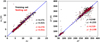 |
Fig. 1 Comparisons of ∆ν and ∆P provided by Vrard et al. (2016) (X-axis) using Kepler data with those derived using our neural network model (Y-axis) for 1800 training (black dots) and 862 testing stars (red dots). The values of the mean and standard deviation of the differences are labelled in the bottom-right corner of each panel. |
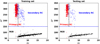 |
Fig. 2 Stellar distributions on the plane of ∆ν–∆P derived using our neural network method for 1800 training (left panel) and 862 testing stars (right panel). The black, red, and blue dots show the 826 RGBs, 1599 primary RCs, and 237 secondary RCs classified by Vrard et al. (2016) using Kepler data, respectively. The blue dashed line (∆P = 150 s) is plotted to separate RGBs and RCs. The black dashed line (∆ν = 5µHz) is plotted to separate primary RCs and secondary RCs. |
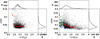 |
Fig. 3 Distributions of 3220 RGBs (left panels) and 3276 RCs common to LAMOST and Kepler (right panels) on the M–∆M/M plane. M and ∆M are the estimated masses and their associated uncertainties. The red dot presents the median values in each mass bin with a bin size of 0.1 M⊙. Green dots are stars with M < 0.7 M⊙. Blue stars show the post-mass-transfer helium-burning stars identified by Li et al. (2022b). Distributions of masses and their associated uncertainties are over-plotted using histograms. |
4 Ages and masses of RGBs and RCs
In this section, we preset our estimations of the masses and ages of our RGBs, primary RCs, and secondary RCs selected from the LAMOST low-resolution spectroscopic survey. To this end, we first estimated the masses and ages using the respective asteroseismic information and isochrone fitting method for LAMOST-Kepler giant stars. We then estimated masses and ages for all LAMOST DR8 giant stars using our neural network method, taking the LAMOST-Kepler giant stars as the training set. For both RGBs and RCs, we built up two different neural network models to estimate ages and masses, respectively.
4.1 Ages and masses of LAMOST-Kepler training and testing stars
Masses of RGBs and RCs can be accurately measured from the asteroseismic information obtained by the Kepler mission. We cross-matched our RGB and RC samples to the Kepler sample with accurate asteroseismic parameters measured by Yu et al. (2018), using light curves of stars provided by the Kepler mission. In total, 3220 and 3276 common RGBs and RCs are found with high-quality spectra (S/N > 50), well-derived spectroscopy, and precise asteroseismic parameters.
For these RGB and RC common stars, we determined their asteroseismic masses using modified scaling relations,
 (2)
(2)
where the Solar values of Teff,⊙, νmax,⊙, and ∆ν⊙ are 5777K, 3090 µHz, and 135.1 µHz (Huber et al. 2011), respectively, and the correction factor ƒ∆ν can be obtained for all stars using the publicly available code Asƒgrid11 provided by Sharma et al. (2016). With this modified scaling relation, the masses of these 3220 and 3276 RGB and RC common stars are derived with precise ∆ν and νmax provided by Yu et al. (2018) and effective temperature Teff taken from Wang et al. (2022). Figure 3 shows the mass distributions estimated from the asteroseismic and spectroscopic stellar atmospheric parameters, as well as their associated uncertainties. The plot clearly shows that the typical uncertainties on the masses of RGBs and RCs are respectively 4.1 and 8.4%.
There are several stars with a mass lower than 0.7 M⊙ as shown in Fig. 3, especially for RCs. Some of these stars may be post-mass-transfer helium-burning stars (Li et al. 2022b), which may be in binary systems, and may have suffered a mass-transfer history with a mass-loss of about 0.1–0.2 M⊙. We cross-matched these stars to the list of post-mass-transfer helium-burning red giants provided by Li et al. (2022b) and find 12 common stars, 9 of them with M < 0.7 M⊙. In the current work, we did not consider such an extreme mass-loss case and readers should therefore be wary of the parameters that we provide for any star with a mass of lower than 0.7 M⊙.
We further estimate the ages of these common stars based on the stellar isochrone fitting method using the aforementioned estimated masses and the effective temperatures, metallicities, and surface gravities provided by Wang et al. (2022). Similar to Huang et al. (2020), we adopt the PARSEC isochrones calculated with a mass-loss parameter ηReimers = 0.2 (Bressan et al. 2012) as the stellar evolution tracks. Here, we adopt one Bayesian approach similar to Xiang et al. (2017) and Huang et al. (2020) when performing isochrone fitting. The mass M, effective temperature Teff, metallicity [M/H], and surface gravity log g are the input constraints.
The posterior probability distributions as a function of age for three stars of typical ages for both RGB and RC stars are shown in Fig. 4. As shown in Fig. 4, we find that the age distributions show prominent peaks, which suggests that the resultant ages are well constrained, especially thanks to the precise mass estimates from asteroseismology information. Figure 5 shows the distributions of the ages of RGBs and RCs, with uncertainties, estimated using the isochrone fitting method. Both the RGB and RC samples cover a whole range of possible ages of stars, from close to zero to 13 Gyr (close to the age of the Universe). The typical age uncertainties on RGB and RC stars are 14 and 23%, respectively. Only a small fraction of stars have age uncertainties of greater than 40%. The larger age uncertainties on RCs compared to RGBs are due to the larger mass uncertainties on RCs. We note that the relationship between age and its associated uncertainty on RGBs is opposite to that for RCs at τ < 8 Gyr, which may be the consequence of the larger variation in mass uncertainty on RCs compared to that of RGBs at 1.0 < M < 1.5 M⊙. The mass uncertainty decreases by 1.7% and 0.02% when masses decrease from 1.55 M⊙ (τ ~ 2.0 Gyr) to 1.05 M⊙ (τ ~ 9.0 Gyr) for RCs and RGBs, respectively. Large mass uncertainties lead to large age uncertainties (∆τ), and therefore older RGBs and RCs have respectively smaller and larger relative age uncertainties (∆τ/т).
After estimating the masses and ages of these 3103 and 3114 RGB and RC stars common to LAMOST and Kepler, we divide each of these samples of stars into two subsamples, a training and a testing subsample. The training samples of RGBs and RCs contain 1493 and 2499 stars, respectively. A further 1610 RGBs and 615 RCs form the testing samples. When selecting training stars, we try to keep a similar number of training stars in each age bin. Nevertheless, as shown in Fig. 5, the RGB sample contains fewer old stars as compared to the RC sample. This is the same for the training set. Figure 6 shows the distributions of the RGB and RC training samples and testing samples on the [M/H]–[α/Fe] plane, colour-coded by mass and age.
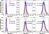 |
Fig. 4 Posterior probability distribution as a function of age for three stars of typical ages for both RGB (top panels) and RC (bottom panels) stars. The blue solid lines denote the median values of the stellar ages. The blue dashed lines show the standard deviations of the stellar ages. The KIC number is given here for the six stars. |
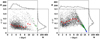 |
Fig. 5 Distributions of 3220 RGBs (left panels) and 3276 RCs common to LAMOST and Kepler (right panels) on the τ–∆τ/τ plane. Here, τ and ∆τ are the estimated ages using the isochrone fitting method and their associated uncertainties. The red dot presents the median value in each age bin with a bin size of 1.0 Gyr. Green dots are stars with M < 0.7 M⊙. Blue star symbols show post-mass-transfer helium-burning stars identified by Li et al. (2022b). Distributions of ages and their associated uncertainties are over-plotted using histograms. |
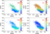 |
Fig. 6 Distributions of 1493 training RGB stars (left panels) and 2499 training RC stars common to LAMOST and Kepler (right panels) on the [Fe/H]-[α/Fe] plane colour-coded according to stellar age (top panels) and mass (bottom panels). Here, the values of [Fe/H] and [α/Fe] come from the value-added catalogue of LAMOST DR8 (Wang et al. 2022). |
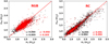 |
Fig. 7 Comparisons of masses estimated with the scaling relation (MS) in Sect. 4.1 and those derived using our neural network model (MNN) using LAMOST spectra for RGB (left panel) and RC stars common to LAMOST and Kepler (right panel) (testing sample: red dots – 1610 RGBs, 615 RCs, and training sample: black dots – 1493 RGBs, 2499 RCs). The µ and σ are the mean and standard deviations of (MS – MNN)/MS, as marked in the bottom-right corner of each panel. |
4.2 Age and mass determinations of RGB and RC stars in LAMOST DR8
After building up the training and testing stars with accurate masses and ages, we derived masses and ages of RGB and RC stars from the LAMOST DR8 spectra using our neural network method, the details of which are provided in Sect. 3.1. The aforementioned RGB and RC training stars are adopted as training samples. Once the LAMOST spectra of all the training and testing stars were pre-processed, following the same procedure as that of Wang et al. (2022), we proceeded to develop a neural network model. This model aimed to establish the connection between the pre-processed LAMOST spectra and the mass/age for RGBs and RCs. Our neural network models used to estimate masses and ages also contain three layers; the total number of neurons for the first, second, and third layers are respectively 512, 256, and 64, which is the same as the neural network model used to estimate asteroseismic parameters in Sect. 3.
Figure 7 shows the comparison of masses estimated with the scaling relation (MS) in Sect. 4.1 with those derived by our neural network model (MNN) using LAMOST spectra for testing RGB and RC stars. We find MNN to be a good match to MS for individual stars. The systematic uncertainties are very small, and the standard deviations of estimated mass are 10% and 9.6% for RGBs and RCs, respectively. Figure 8 shows the comparison of ages estimated with the isochrone fitting method (τISO) in Sect. 4.1 with those derived by our neural network model (τNN) using LAMOST spectra for testing RGB and RC stars. We find that τNN is consistent with τISO for individual stars. The τNN are overestimated by about 10% for RGB stars. The systematic uncertainties on τNN for RCs are very small. The standard deviations of estimated age are 30% and 24% for RGBs and RCs, respectively. Figures 7 or 8 also show the comparisons between MNN and MS and between τNN and τISO for training stars. The MNN (τNN) is in good agreement with MS (τISO). The standard deviations of estimated mass are respectively 5.9% and 9.4% for RGB and RC training stars. For age estimates of RGB and RC training stars, the standard deviations are 26.6% and 19.4%, respectively. In summary, our neural networks could derive precise mass and age for RGB and RC stars from LAMOST spectra. Finally, below, we adopt our neural network models to 937082, 244458, and 167105 RGB, primary RC, and secondary RC stellar spectra and derive their spectroscopic masses and ages.
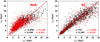 |
Fig. 8 Comparisons of age estimated with isochrone fitting (τISO) in Sect. 4.1 and age derived by our neural network model (τNN) using LAMOST spectra for 3103 RGB (left panel) and RC (right panel) stars common to LAMOST and Kepler (testing sample: red dots – 1610 RGBs, 615 RCs, and training sample: black dots – 1493 RGBs, 2499 RCs). The µ and σ are the mean and standard deviations of (τIS0 – τNN)/τIS0, as marked in the bottom-right corner of each panel. |
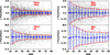 |
Fig. 9 Relative internal residuals of our masses (left panels) and ages (right panels) estimated using spectra given by duplicate observations with similar spectral S/N for LAMOST RGB (top panels) and RC (bottom panels) stars. Black dots are the differences of duplicate observations of S/N differences smaller than 10%. Blue dots and error bars represent the median values and standard deviations (after dividing by |

5 Validation of the spectroscopic masses and ages of RGBs and RCs
In this section, we first examine the uncertainties on the masses and ages of RGBs and RCs using our neural network method through internal comparisons. Secondly, through external comparisons, we further examine the uncertainties, including the systematic biases affecting masses and ages.
5.1 The uncertainties on estimated masses and ages of RGBs and RCs
The uncertainties of estimated masses and ages depend on the spectral noise (random uncertainties) and method uncertainties. As discussed in Huang et al. (2020) and Wang et al. (2022), the random uncertainties on masses and ages are estimated by comparing results derived from duplicate observations of similar spectral S/Ns (differing by less than 10 per cent) collected during different nights. The relative residuals of mass and age estimates (after dividing by  ) along with mean spectral S/Ns are shown in Fig. 9. To properly obtain random uncertainties on age and mass, we fitted the relative residuals with the equation used by Huang et al. (2020):
 (3)
(3)
where σr represents the random uncertainty. In addition to the random uncertainties, method uncertainties (σm) are also considered when we estimate the uncertainties on stellar parameters. The final uncertainties are given by  . The method uncertainties are provided by the relative residuals between our estimated results and the asteroseismic results of the training sample. For the ages and masses of RGB stars, the method uncertainties are 26.6 and 5.9%, as shown in Figs. 7 and 8, respectively. The method uncertainties of age and mass are 19.4 and 9.4% for RC stars, as shown in Figs. 7 and 8, respectively.
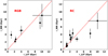 |
Fig. 10 Comparisons of our estimated ages (τNN) of open clusters with literature values (τLIT) for LAMOST RGBs (left panel) and RCs (right panel). |
Age values of open clusters estimated using our neural network and ages of literature values for both LAMOST RGB and RC stars.
5.2 The ages of members of open clusters
Stars in open clusters are believed to form almost simultaneously from a single gas cloud and are therefore expected to have almost the same age, metallicity, distance, and kinematics. Open clusters are therefore useful for testing the accuracy of ages. Zhong et al. (2020a,b) provide 8811 cluster members of 295 clusters observed by LAMOST. These latter authors cross-matched the open cluster catalogue and the member stars provided by Cantat-Gaudin et al. (2018) with LAMOST DR5. Amongst these clusters, we carefully selected open clusters with a wide age range (1–10 Gyr) in order to check our age estimates. As shown in Fig. 10, we find that our ages of open clusters are consistent with those in the literature for both RGB and RC stars of all ages, from young (~ 2 Gyr) to old (~ 10 Gyr). Table 1 presents our age estimates and literature age values.
5.3 Comparison of masses and ages of RGB and RC stars with previous results
A catalogue containing accurate stellar ages for ~0.64 million RGB stars of LAMOST DR4 was published by Wu et al. (2019). Furthermore, Sanders & Das (2018) determined distances and ages for ~3 million stars with astrometric information from Gaia DR2 and spectroscopic parameters from massive spectro-scopic surveys: including the APOGEE, Gaia-ESO, GALAH, LAMOST, RAVE, and SEGUE surveys. We cross-matched our catalogue with the catalogues of Wu et al. (2019) and Sanders & Das (2018) and obtain ~97 000 and 83 000 common RGB stars (S/N ≥ 50, 2.0 < log g < 3.2 dex, 4000 < Teff < 5500 K) with the catalogues of Wu et al. (2019) and Sanders & Das (2018), respectively. The comparisons are shown in Fig. 11. Generally, our ages are younger than those estimated by Wu et al. (2019). In particular, for stars towards the older end of the range of RGB and RCs analysed here, our ages are younger than the ages of Wu et al. (2019) by 2–3 Gyr. This is mainly due to the different choices of isochrone database between this work and Wu et al. (2019); we adopt the isochrones from PARSEC and these latter authors use those of Yonsei–Yale (Y2; Demarque et al. 2004), respectively. The lack of old (low-mass: M < 1.0 M⊙) RGB training stars in this work may also be factor driving our lower age estimates. Our estimated ages could agree well with those estimated by Sanders & Das (2018).
Montalbán et al. (2021) provided precise stellar ages (~11%) and masses for 95 RGBs observed by the Kepler space mission by combining asteroseismology with kinematics and chemical abundances of stars. There are 62 stars in common between our catalogue and their list. As shown in Fig. 12, ages of old stars with τ > 8 Gyr are underestimated by 2–3 Gyr compared to the results of Montalbán et al. (2021), because masses of these stars are overestimated by ~ 0.1M⊙. Montalbán et al. (2021) estimate masses by adopting the individual frequencies of radial modes as observational constraints, which may provide more accurate masses (Lebreton & Goupil 2014; Miglio et al. 2017; Rendle et al. 2019; Montalbán et al. 2021). Building up a training sample containing enough RGBs with accurate age and mass estimates by adopting individual frequencies as observational constraints may dramatically improve the determination of age and mass for RGBs using machine learning methods. A potential challenge is the lack of precise individual frequencies for a larger sample size of red giant stars (~2000–6000 stars). Nevertheless, this method is beyond the scope of the present paper.
In a previous study, we determined precise distances, masses, ages, and 3D velocities for ~ 140 000 primary RCs selected from the LAMOST database (Huang et al. 2020). The catalogue of Sanders & Das (2018) also contains a great many RC stars with age estimates. Our catalogue contains ~ 52 000 and 72 000 RC stars (S/N ≥ 50) in common with the catalogues of Huang et al. (2020) and Sanders & Das (2018), respectively. Figure 13 shows a comparison between the ages derived in this work and the ages provided by Huang et al. (2020) and Sanders & Das (2018) for RC stars. Our ages are highly consistent with those of Huang et al. (2020). The ages in this work are generally consistent with those of Sanders & Das (2018), although a mild offset of 2–3 Gyr (our values minus those of Sanders & Das 2018) is detected.
In summary, we calculate, via internal comparisons, uncertainties on ages and masses of RC stars of smaller than 25 and 10%, respectively, for stars with spectral S/N > 50. For RGB stars with spectral S/N > 50, we calculate uncertainties on ages and masses of smaller than 20 and 8%, respectively. Comparison of the ages derived in this work with those from the literature for open cluster member stars reveals very small systematic uncertainties on our age estimates for both RGB and RC stars. Our age estimations are a close match to those of Sanders & Das (2018) for RGB stars and to those of Huang et al. (2020) for RC stars.
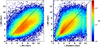 |
Fig. 11 Comparisons of our estimated ages with those provided by Wu et al. (2019, left panel) and Sanders & Das (2018, right panel) for 97 112 and 83 199 RGB stars with S/Ns > 50 and common to our sample, respectively. |
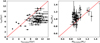 |
Fig. 12 Comparisons of our estimated ages and masses with those provided by Montalbán et al. (2021) for 62 common RGB stars. |
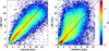 |
Fig. 13 Comparisons of our estimated ages with those provided by Huang et al. (2020, left panel) and Sanders & Das (2018, right panel) for 42 969 and 52 944 RC stars with S/Ns > 50 and common to our sample, respectively. |
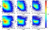 |
Fig. 14 Stellar number density distributions of the 520 073 unique LAMOST RGB (left panels), 154 587 unique primary RC (middle panels) and 66 395 unique secondary RC (right panels) stars with spectral S/Ns > 20 on the X–Y (top panels) and X–Z (bottom panels) planes in Galactic Cartesian coordinates. |
6 Properties of the LAMOST RGB and RC samples
In addition to estimating accurate masses and ages, we also provide stellar atmospheric parameters (Teff, log g and [Fe/H]), chemical element abundance ratios ([M/H], [α/M], [C/Fe] and [N/Fe]), the absolute magnitudes of 14 bands (MG, MBp, MRp of Gaia bands, MJ, MH, MKs of 2MASS bands, MW1, MW2 of WISE bands, MB, MV,  of APASS bands and Mg, Mr, Mi of SDSS bands), and photometric distances for all these RGBs, primary RCs, and secondary RCs, which are taken from the value-added catalogue of LAMOSTDR8 built up by Wang et al. (2022). We were therefore able to study the spatial coverage and age distributions on the R–Z plane and on the [Fe/H]–[α/Fe] plane of our RGB, primary RC, and secondary RC samples.
Figure 14 shows the stellar number density distributions of our RGB, primary RC, and secondary RC stellar samples on the X–Y and X–Z planes, which cover a large volume of the Milky Way (5 < R < 20 kpc and |Z| < 5 kpc). One can use these distributions to probe the structural, chemical, and kinematic properties of the Galactic thin and thick discs and the halo by combining this information with the proper motions provided by Gaia DR3 (Gaia Collaboration 2023a; Babusiaux et al. 2023).
The age distributions of RGB, primary RC, and secondary RC stars on the R–Z plane are presented in Fig. 15. From this figure, we can see that there are negative age gradients in the radial direction and positive age gradients in the vertical direction for both RGB and primary RC stars, which were reported in a series of previous studies (e.g., Martig et al. 2016b; Casagrande et al. 2016). For secondary RCs, there are positive age gradients in the vertical direction. Flat or slightly positive radial age gradients are found for secondary RCs, which may be meaningless considering the small mean age coverage (from ~ 1.1 Gyr at R ~ 9 kpc to 1.5 Gyr at R ~ 12 kpc) and the large age uncertainties for stars of younger ages. The strong flaring of the young Galactic disc (young stellar populations extending to greater heights from the Galactic plane with increasing R) is clearly seen in the age distributions of RGB and primary RC stars. Similar results were also noted by Xiang et al. (2017), Wu et al. (2019), and Huang et al. (2020).
Figure 16 shows the stellar number density and mean age distributions on the [Fe/H]–[α/Fe] plane for the RGB, primary RC, and secondary RC stars. The stellar number density distributions of RGB and primary RC stars suggest that the RGB and primary RC stellar populations could each be clearly separated into two individual sequences, that is, high-α and low-α sequences. The high- and low-α sequences are associated with the so-called chemically thick and thin discs, respectively. For primary RC stellar populations, the mean ages of the high-and low-α sequences are ~ 8 Gyr and ~ 2.5 Gyr, respectively. The high-α sequence is older than the low-α sequence. The results are consistent with previous findings for the solar neighbourhood using high-resolution spectroscopy (Bensby et al. 2003; Haywood 2008; Haywood et al. 2013; Hayden et al. 2015) and results using a large sample of stars with ages derived from the LAMOST low-resolution spectra (Xiang et al. 2017; Wu et al. 2019; Huang et al. 2020). For RGB stellar populations, the ages of high- and low-α sequences are ~6Gyr and ~3 Gyr, respectively. The high-α sequence is older than the low-α sequence with a smaller age difference as compared to that of primary RC stellar populations. For RGB stellar populations, the eldest stellar populations are located in the transition region of high-and low-α sequences. Almost all of the secondary RC stars are thin disc stars, because they are massive young stars.
For both RGB and primary RC stellar populations, there are some stars with a metallicity of higher than 0.2 dex that are also older than stars on the low-α sequence. Some of these stars are the so-called old-yet-metal-rich stars (6 < τ < 8 Gyr, [Fe/H] > 0.2 dex, −0.05 < [α/Fe] < 0.05 dex), and it has been suggested that these stars may come from the inner disc via radial migration processes (Xiang et al. 2015; Wang et al. 2019; Feuillet et al. 2018, 2019; Hasselquist et al. 2019; Boeche et al. 2013; Chen et al. 2019).
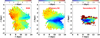 |
Fig. 15 Median age distributions of the 259 372 unique LAMOST RGB (left panels), 92 795 unique primary RC (middle panels) and 28 104 unique secondary RC (right panels) stars with spectral S/Ns > 50 on the R–Z plane. |
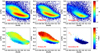 |
Fig. 16 Stellar number density (top panels) and mean age (bottom panels) distributions on the [Fe/H]–[α/Fe] plane for the 259 372 unique LAMOST RGBs (left panels), 92 795 unique primary RCs (middle panels), and 28 104 unique secondary RCs (right panels) with spectral S/Ns > 50. |
7 Summary
In the current work, we build up a catalogue of masses and ages for 937082, 244458, and 167 105 RGBs, primary RCs, and secondary RCs selected from LAMOST DR8 low-resolution stellar spectra of spectral S/N>10. Amongst them, 696680 RGBs, 180436 primary RCs, and 120 907 secondary RCs are unique stars. The RGBs, primary RCs, and secondary RCs are identified using the large frequency spacing (∆v) and period spacing (∆P) estimated using a neural network method. The contaminations of RGB stars by RC stars and contaminations of RCs by RGBs are both about 1% for stars with spectral S/N> 20.
Using relations of stellar spectra and masses and ages built up by the neural network method using the RGB and RC stars in the LAMOST-Kepler fields that have accurate asteroseismic mass and age measurements as training samples, we estimated the masses and ages of all LAMOST RGB and RC stars. The typical uncertainties on estimated masses and ages, as examined by the testing sample, are 10% and 30% for RGB stars, and 9% and 24% for RC stars, respectively.
The RGB and RC stellar populations cover a large volume of the Milky Way (5 < R < 20 kpc and |Z| < 5 kpc). We also provide stellar atmospheric parameters, chemical element abundances, absolute magnitudes for 14 bands, and photometric distances. These can be used to probe the structural, chemical, and kinematic properties of both the Galactic thin and thick discs and the halo through combination with proper motions provided by Gaia DR3. The catalogue is available at the CDS and the LAMOST official website3.
Acknowledgements
This work was funded by the National Key R&D Program of China (No. 2019YFA0405500) and the National Natural Science Foundation of China (NSFC Grant Nos. 12203037, 12173007 and 11973001). We acknowledge the science research grants from the China Manned Space Project with No. CMS-CSST-2021-B03. We used data from the European Space Agency mission Gaia (http://www.cosmos.esa.int/gaia), processed by the Gaia Data Processing and Analysis Consortium (DPAC; see http://www.cosmos. esa.int/web/gaia/dpac/consortium). Guoshoujing Telescope (the Large Sky Area Multi-Object Fiber Spectroscopic Telescope LAMOST) is a National Major Scientific Project built by the Chinese Academy of Sciences. Funding for the project has been provided by the National Development and Reform Commission. LAMOST is operated and managed by the National Astronomical Observatories, Chinese Academy of Sciences.
References
- An, D., Terndrup, D. M., Pinsonneault, M. H., & Lee, J.-W. 2015, ApJ, 811, 46 [NASA ADS] [CrossRef] [Google Scholar]
- Anthony-Twarog, B. J., Deliyannis, C. P., & Twarog, B. A. 2014, AJ, 148, 51 [NASA ADS] [CrossRef] [Google Scholar]
- Babusiaux, C., Fabricius, C., Khanna, S., et al. 2023, A&A, 674, A32 [NASA ADS] [CrossRef] [EDP Sciences] [Google Scholar]
- Bedding, T. R., Mosser, B., Huber, D., et al. 2011, Nature, 471, 608 [Google Scholar]
- Bellinger, E. P. 2020, MNRAS, 492, L50 [Google Scholar]
- Bensby, T., Feltzing, S., & Lundström, I. 2003, A&A, 410, 527 [CrossRef] [EDP Sciences] [Google Scholar]
- Boeche, C., Siebert, A., Piffl, T., et al. 2013, A&A, 559, A59 [NASA ADS] [CrossRef] [EDP Sciences] [Google Scholar]
- Bossini, D., Vallenari, A., Bragaglia, A., et al. 2019, A&A, 623, A108 [NASA ADS] [CrossRef] [EDP Sciences] [Google Scholar]
- Bovy, J., Nidever, D. L., Rix, H.-W., et al. 2014, ApJ, 790, 127 [CrossRef] [Google Scholar]
- Bragaglia, A., Tosi, M., Andreuzzi, G., & Marconi, G. 2006, MNRAS, 368, 1971 [NASA ADS] [CrossRef] [Google Scholar]
- Bressan, A., Marigo, P., Girardi, L., et al. 2012, MNRAS, 427, 127 [NASA ADS] [CrossRef] [Google Scholar]
- Brewer, L. N., Sandquist, E. L., Mathieu, R. D., et al. 2016, AJ, 151, 66 [NASA ADS] [CrossRef] [Google Scholar]
- Cantat-Gaudin, T., Jordi, C., Vallenari, A., et al. 2018, A&A, 618, A93 [NASA ADS] [CrossRef] [EDP Sciences] [Google Scholar]
- Casagrande, L., Silva Aguirre, V., Schlesinger, K. J., et al. 2016, MNRAS, 455, 987 [Google Scholar]
- Chaplin, W. J., & Miglio, A. 2013, ARA&A, 51, 353 [Google Scholar]
- Chen, Y. Q., Zhao, G., Zhao, J. K., et al. 2019, AJ, 158, 249 [NASA ADS] [CrossRef] [Google Scholar]
- Demarque, P., Woo, J.-H., Kim, Y.-C., & Yi, S. K. 2004, ApJS, 155, 667 [NASA ADS] [CrossRef] [Google Scholar]
- Deng, L.-C., Newberg, H. J., Liu, C., et al. 2012, Res. Astron. Astrophys., 12, 735 [Google Scholar]
- De Silva, G. M., Freeman, K. C., Bland-Hawthorn, J., et al. 2015, MNRAS, 449, 2604 [NASA ADS] [CrossRef] [Google Scholar]
- Elsworth, Y., Hekker, S., Basu, S., & Davies, G. R. 2017, MNRAS, 466, 3344 [NASA ADS] [CrossRef] [Google Scholar]
- Feuillet, D. K., Bovy, J., Holtzman, J., et al. 2018, MNRAS, 477, 2326 [NASA ADS] [CrossRef] [Google Scholar]
- Feuillet, D. K., Frankel, N., Lind, K., et al. 2019, MNRAS, 489, 1742 [Google Scholar]
- Gaia Collaboration (Prusti, T., et al.) 2016, A&A, 595, A1 [NASA ADS] [CrossRef] [EDP Sciences] [Google Scholar]
- Gaia Collaboration (Brown, A. G. A., et al.) 2021, A&A, 649, A1 [NASA ADS] [CrossRef] [EDP Sciences] [Google Scholar]
- Gaia Collaboration (Arenou, F., et al.) 2023a, A&A, 674, A34 [CrossRef] [EDP Sciences] [Google Scholar]
- Gaia Collaboration (Recio-Blanco, A., et al.) 2023b, A&A, 674, A38 [CrossRef] [EDP Sciences] [Google Scholar]
- Hasselquist, S., Holtzman, J. A., Shetrone, M., et al. 2019, ApJ, 871, 181 [NASA ADS] [CrossRef] [Google Scholar]
- Hawkins, K., Ting, Y.-S., & Walter-Rix, H. 2018, ApJ, 853, 20 [NASA ADS] [CrossRef] [Google Scholar]
- Hayden, M. R., Bovy, J., Holtzman, J. A., et al. 2015, ApJ, 808, 132 [Google Scholar]
- Haywood, M. 2008, MNRAS, 388, 1175 [NASA ADS] [CrossRef] [Google Scholar]
- Haywood, M., Di Matteo, P., Lehnert, M. D., Katz, D., & Gómez, A. 2013, A&A, 560, A109 [NASA ADS] [CrossRef] [EDP Sciences] [Google Scholar]
- Ho, A. Y. Q., Ness, M. K., Hogg, D. W., et al. 2017, ApJ, 836, 5 [NASA ADS] [CrossRef] [Google Scholar]
- Huang, Y., Liu, X.-W., Zhang, H.-W., et al. 2015, Res. Astron. Astrophys., 15, 1240 [CrossRef] [Google Scholar]
- Huang, Y., Schönrich, R., Zhang, H., et al. 2020, ApJS, 249, 29 [NASA ADS] [CrossRef] [Google Scholar]
- Huber, D., Bedding, T. R., Stello, D., et al. 2011, ApJ, 743, 143 [Google Scholar]
- Huber, D., Silva Aguirre, V., Matthews, J. M., et al. 2014, ApJS, 211, 2 [NASA ADS] [CrossRef] [Google Scholar]
- Kharchenko, N. V., Piskunov, A. E., Schilbach, E., Röser, S., & Scholz, R. D. 2013, A&A, 558, A53 [NASA ADS] [CrossRef] [EDP Sciences] [Google Scholar]
- Lebreton, Y., & Goupil, M. J. 2014, A&A, 569, A21 [NASA ADS] [CrossRef] [EDP Sciences] [Google Scholar]
- Li, T., Bedding, T. R., Christensen-Dalsgaard, J., et al. 2020, MNRAS, 495, 3431 [Google Scholar]
- Li, T., Li, Y., Bi, S., et al. 2022a, ApJ, 927, 167 [NASA ADS] [CrossRef] [Google Scholar]
- Li, Y., Bedding, T. R., Murphy, S. J., et al. 2022b, Nat. Astron., 6, 673 [NASA ADS] [CrossRef] [Google Scholar]
- Liu, X.-W., Yuan, H.-B., Huo, Z.-Y., et al. 2014, in IAU Symposium, 298, IAU Symposium, eds. S. Feltzing, G. Zhao, N. A. Walton, & P. Whitelock, 310 [Google Scholar]
- Luo, A. L., Zhao, Y.-H., Zhao, G., et al. 2015, Res. Astron. Astrophys., 15, 1095 [Google Scholar]
- Majewski, S. R., Schiavon, R. P., Frinchaboy, P. M., et al. 2017, AJ, 154, 94 [NASA ADS] [CrossRef] [Google Scholar]
- Martell, S. L., Smith, G. H., & Briley, M. M. 2008, AJ, 136, 2522 [NASA ADS] [CrossRef] [Google Scholar]
- Martig, M., Fouesneau, M., Rix, H.-W., et al. 2016a, MNRAS, 456, 3655 [NASA ADS] [CrossRef] [Google Scholar]
- Martig, M., Minchev, I., Ness, M., Fouesneau, M., & Rix, H.-W. 2016b, ApJ, 831, 139 [CrossRef] [Google Scholar]
- Masseron, T., & Gilmore, G. 2015, MNRAS, 453, 1855 [CrossRef] [Google Scholar]
- Masseron, T., & Hawkins, K. 2017, A&A, 597, A3 [NASA ADS] [CrossRef] [EDP Sciences] [Google Scholar]
- Masseron, T., Lagarde, N., Miglio, A., Elsworth, Y., & Gilmore, G. 2017, MNRAS, 464, 3021 [NASA ADS] [CrossRef] [Google Scholar]
- Miglio, A., Chiappini, C., Mosser, B., et al. 2017, Astron. Nachr., 338, 644 [Google Scholar]
- Molenda-Zakowicz, J., Brogaard, K., Niemczura, E., et al. 2014, MNRAS, 445, 2446 [CrossRef] [Google Scholar]
- Montalbán, J., Miglio, A., Noels, A., Scuflaire, R., & Ventura, P. 2010, ApJ, 721, L182 [Google Scholar]
- Montalbán, J., Mackereth, J. T., Miglio, A., et al. 2021, Nat, Astron., 5, 640 [CrossRef] [Google Scholar]
- Mosser, B., Barban, C., Montalbán, J., et al. 2011, A&A, 532, A86 [NASA ADS] [CrossRef] [EDP Sciences] [Google Scholar]
- Mosser, B., Goupil, M. J., Belkacem, K., et al. 2012, A&A, 540, A143 [NASA ADS] [CrossRef] [EDP Sciences] [Google Scholar]
- Ness, M., Hogg, D. W., Rix, H. W., et al. 2016, ApJ, 823, 114 [NASA ADS] [CrossRef] [Google Scholar]
- Pinsonneault, M. H., Elsworth, Y., Epstein, C., et al. 2014, ApJS, 215, 19 [Google Scholar]
- Recio-Blanco, A., de Laverny, P., Palicio, P. A., et al. 2023, A&A, 674, A29 [NASA ADS] [CrossRef] [EDP Sciences] [Google Scholar]
- Rendle, B. M., Buldgen, G., Miglio, A., et al. 2019, MNRAS, 484, 771 [Google Scholar]
- Salaris, M., Weiss, A., & Percival, S. M. 2004, A&A, 414, 163 [NASA ADS] [CrossRef] [EDP Sciences] [Google Scholar]
- Sanders, J. L., & Das, P. 2018, MNRAS, 481, 4093 [CrossRef] [Google Scholar]
- Sandquist, E. L., Jessen-Hansen, J., Shetrone, M. D., et al. 2016, ApJ, 831, 11 [Google Scholar]
- Sharma, S., Stello, D., Bland-Hawthorn, J., Huber, D., & Bedding, T. R. 2016, ApJ, 822, 15 [Google Scholar]
- Soderblom, D. R. 2010, ARA&A, 48, 581 [Google Scholar]
- Steinmetz, M., Zwitter, T., Siebert, A., et al. 2006, AJ, 132, 1645 [Google Scholar]
- Stello, D., Huber, D., Bedding, T. R., et al. 2013, ApJ, 765, L41 [CrossRef] [Google Scholar]
- Stello, D., Vanderburg, A., Casagrande, L., et al. 2016, ApJ, 832, 133 [NASA ADS] [CrossRef] [Google Scholar]
- Tayar, J., Somers, G., Pinsonneault, M. H., et al. 2017, ApJ, 840, 17 [NASA ADS] [CrossRef] [Google Scholar]
- Ting, Y.-S., Hawkins, K., & Rix, H.-W. 2018, ApJ, 858, L7 [NASA ADS] [CrossRef] [Google Scholar]
- Vrard, M., Mosser, B., & Samadi, R. 2016, A&A, 588, A87 [CrossRef] [EDP Sciences] [Google Scholar]
- Wang, C., Liu, X. W., Xiang, M. S., et al. 2019, MNRAS, 482, 2189 [NASA ADS] [CrossRef] [Google Scholar]
- Wang, C., Huang, Y., Yuan, H., et al. 2022, ApJS, 259, 51 [NASA ADS] [CrossRef] [Google Scholar]
- Wu, Y., Xiang, M., Bi, S., et al. 2018, MNRAS, 475, 3633 [NASA ADS] [CrossRef] [Google Scholar]
- Wu, Y., Xiang, M., Zhao, G., et al. 2019, MNRAS, 484, 5315 [NASA ADS] [CrossRef] [Google Scholar]
- Wu, Y., Xiang, M., Zhao, G., et al. 2023, MNRAS, 520, 1913 [CrossRef] [Google Scholar]
- Xiang, M.-S., Liu, X.-W., Yuan, H.-B., et al. 2015, Res. Astron. Astrophys., 15, 1209 [CrossRef] [Google Scholar]
- Xiang, M., Liu, X., Shi, J., et al. 2017, ApJS, 232, 2 [NASA ADS] [CrossRef] [Google Scholar]
- Yang, W., Meng, X., Bi, S., et al. 2012, MNRAS, 422, 1552 [NASA ADS] [CrossRef] [Google Scholar]
- Yanny, B., Rockosi, C., Newberg, H. J., et al. 2009, AJ, 137, 4377 [Google Scholar]
- Yu, J., Huber, D., Bedding, T. R., et al. 2018, ApJS, 236, 42 [NASA ADS] [CrossRef] [Google Scholar]
- Zhao, G., Zhao, Y.-H., Chu, Y.-Q., Jing, Y.-P., & Deng, L.-C. 2012, Res. Astron. Astrophys., 12, 723 [NASA ADS] [CrossRef] [Google Scholar]
- Zhong, J., Chen, L., Wu, D., et al. 2020a, A&A, 640, A127 [NASA ADS] [CrossRef] [EDP Sciences] [Google Scholar]
- Zhong, J., Chen, L., Wu, D., et al. 2020b, VizieR Online Data Catalog: J/A+A/640/A127 [Google Scholar]
The primary RC stars are helium-burning (ignited non-degenerately) descendants of low-mass stars (typically smaller than 2 M⊙), while the secondary RC stars are helium-burning descendants of high-mass stars (typically larger than 2 M⊙).
All Tables
Age values of open clusters estimated using our neural network and ages of literature values for both LAMOST RGB and RC stars.
All Figures
|
Fig. 1 Comparisons of ∆ν and ∆P provided by Vrard et al. (2016) (X-axis) using Kepler data with those derived using our neural network model (Y-axis) for 1800 training (black dots) and 862 testing stars (red dots). The values of the mean and standard deviation of the differences are labelled in the bottom-right corner of each panel. |
| In the text | |
|
Fig. 2 Stellar distributions on the plane of ∆ν–∆P derived using our neural network method for 1800 training (left panel) and 862 testing stars (right panel). The black, red, and blue dots show the 826 RGBs, 1599 primary RCs, and 237 secondary RCs classified by Vrard et al. (2016) using Kepler data, respectively. The blue dashed line (∆P = 150 s) is plotted to separate RGBs and RCs. The black dashed line (∆ν = 5µHz) is plotted to separate primary RCs and secondary RCs. |
| In the text | |
|
Fig. 3 Distributions of 3220 RGBs (left panels) and 3276 RCs common to LAMOST and Kepler (right panels) on the M–∆M/M plane. M and ∆M are the estimated masses and their associated uncertainties. The red dot presents the median values in each mass bin with a bin size of 0.1 M⊙. Green dots are stars with M < 0.7 M⊙. Blue stars show the post-mass-transfer helium-burning stars identified by Li et al. (2022b). Distributions of masses and their associated uncertainties are over-plotted using histograms. |
| In the text | |
|
Fig. 4 Posterior probability distribution as a function of age for three stars of typical ages for both RGB (top panels) and RC (bottom panels) stars. The blue solid lines denote the median values of the stellar ages. The blue dashed lines show the standard deviations of the stellar ages. The KIC number is given here for the six stars. |
| In the text | |
|
Fig. 5 Distributions of 3220 RGBs (left panels) and 3276 RCs common to LAMOST and Kepler (right panels) on the τ–∆τ/τ plane. Here, τ and ∆τ are the estimated ages using the isochrone fitting method and their associated uncertainties. The red dot presents the median value in each age bin with a bin size of 1.0 Gyr. Green dots are stars with M < 0.7 M⊙. Blue star symbols show post-mass-transfer helium-burning stars identified by Li et al. (2022b). Distributions of ages and their associated uncertainties are over-plotted using histograms. |
| In the text | |
|
Fig. 6 Distributions of 1493 training RGB stars (left panels) and 2499 training RC stars common to LAMOST and Kepler (right panels) on the [Fe/H]-[α/Fe] plane colour-coded according to stellar age (top panels) and mass (bottom panels). Here, the values of [Fe/H] and [α/Fe] come from the value-added catalogue of LAMOST DR8 (Wang et al. 2022). |
| In the text | |
|
Fig. 7 Comparisons of masses estimated with the scaling relation (MS) in Sect. 4.1 and those derived using our neural network model (MNN) using LAMOST spectra for RGB (left panel) and RC stars common to LAMOST and Kepler (right panel) (testing sample: red dots – 1610 RGBs, 615 RCs, and training sample: black dots – 1493 RGBs, 2499 RCs). The µ and σ are the mean and standard deviations of (MS – MNN)/MS, as marked in the bottom-right corner of each panel. |
| In the text | |
|
Fig. 8 Comparisons of age estimated with isochrone fitting (τISO) in Sect. 4.1 and age derived by our neural network model (τNN) using LAMOST spectra for 3103 RGB (left panel) and RC (right panel) stars common to LAMOST and Kepler (testing sample: red dots – 1610 RGBs, 615 RCs, and training sample: black dots – 1493 RGBs, 2499 RCs). The µ and σ are the mean and standard deviations of (τIS0 – τNN)/τIS0, as marked in the bottom-right corner of each panel. |
| In the text | |
|
Fig. 9 Relative internal residuals of our masses (left panels) and ages (right panels) estimated using spectra given by duplicate observations with similar spectral S/N for LAMOST RGB (top panels) and RC (bottom panels) stars. Black dots are the differences of duplicate observations of S/N differences smaller than 10%. Blue dots and error bars represent the median values and standard deviations (after dividing by |
| In the text | |
|
Fig. 10 Comparisons of our estimated ages (τNN) of open clusters with literature values (τLIT) for LAMOST RGBs (left panel) and RCs (right panel). |
| In the text | |
|
Fig. 11 Comparisons of our estimated ages with those provided by Wu et al. (2019, left panel) and Sanders & Das (2018, right panel) for 97 112 and 83 199 RGB stars with S/Ns > 50 and common to our sample, respectively. |
| In the text | |
|
Fig. 12 Comparisons of our estimated ages and masses with those provided by Montalbán et al. (2021) for 62 common RGB stars. |
| In the text | |
|
Fig. 13 Comparisons of our estimated ages with those provided by Huang et al. (2020, left panel) and Sanders & Das (2018, right panel) for 42 969 and 52 944 RC stars with S/Ns > 50 and common to our sample, respectively. |
| In the text | |
|
Fig. 14 Stellar number density distributions of the 520 073 unique LAMOST RGB (left panels), 154 587 unique primary RC (middle panels) and 66 395 unique secondary RC (right panels) stars with spectral S/Ns > 20 on the X–Y (top panels) and X–Z (bottom panels) planes in Galactic Cartesian coordinates. |
| In the text | |
|
Fig. 15 Median age distributions of the 259 372 unique LAMOST RGB (left panels), 92 795 unique primary RC (middle panels) and 28 104 unique secondary RC (right panels) stars with spectral S/Ns > 50 on the R–Z plane. |
| In the text | |
|
Fig. 16 Stellar number density (top panels) and mean age (bottom panels) distributions on the [Fe/H]–[α/Fe] plane for the 259 372 unique LAMOST RGBs (left panels), 92 795 unique primary RCs (middle panels), and 28 104 unique secondary RCs (right panels) with spectral S/Ns > 50. |
| In the text | |
Current usage metrics show cumulative count of Article Views (full-text article views including HTML views, PDF and ePub downloads, according to the available data) and Abstracts Views on Vision4Press platform.
Data correspond to usage on the plateform after 2015. The current usage metrics is available 48-96 hours after online publication and is updated daily on week days.
Initial download of the metrics may take a while.