| Issue |
A&A
Volume 674, June 2023
|
|
|---|---|---|
| Article Number | A182 | |
| Number of page(s) | 15 | |
| Section | The Sun and the Heliosphere | |
| DOI | https://doi.org/10.1051/0004-6361/202345999 | |
| Published online | 19 June 2023 | |
Hale cycle in solar hemispheric radio flux and sunspots: Evidence for a northward-shifted relic field
Space Climate Group, Space Physics and Astronomy Research Unit, University of Oulu, PO Box 8000 90014 Oulu, Finland
e-mail: This email address is being protected from spambots. You need JavaScript enabled to view it.
Received:
25
January
2023
Accepted:
30
April
2023
Abstract
Context. Solar and heliospheric parameters occasionally depict notable differences between the northern and southern solar hemisphere. Although the hemispheric asymmetries of some heliospheric parameters vary systematically with the Hale cycle, this has not been found to be commonly valid for solar parameters. Also, no verified physical mechanism exists that can explain possible systematic hemispheric asymmetries.
Aims. We use a novel method of high heliolatitudinal vantage points to increase the fraction of one hemisphere in solar 10.7 cm radio fluxes and sunspot numbers. We aim to explore the possibility that solar radio fluxes and sunspot numbers, the two most fundamental solar parameters, depict systematic, possibly mutually similar patterns in their hemispheric activities during the last 75 yr.
Methods. We used three different sets of time intervals with increasing mean heliographic latitude and calculated corresponding hemispheric high-latitude radio fluxes and sunspot numbers. We also normalized these fluxes by yearly means in order to study the variation of fluxes in the two hemispheres over the whole 75 yr time interval.
Results. We find that cycle-maximum radio fluxes and sunspot numbers in each odd solar cycle (19, 21, 23) are larger at northern high latitudes than at southern high latitudes, while maximum fluxes and numbers in all even cycles (18, 20, 22 24) are larger at southern high latitudes than at northern high latitudes. This alternation indicates a new form of systematic, Hale-cycle-related variation in solar activity. Hemispheric differences at cycle maxima are 15% for radio flux and 23% for sunspot numbers, on average. The difference is largest during cycle 19 and smallest in cycle 24. Normalized radio fluxes depict a dominant Hale-cycle variation in both hemispheres, with an opposite phase and overall amplitude of about 5% in the north and 4% in the south. Thus, there is systematic Hale-cycle alternation in magnetic flux emergence in both hemispheres.
Conclusions. The hemispheric Hale cycle in flux emergence can be explained if there is a northward-directed relic magnetic field, which is slightly shifted northward. In that case, in odd cycles, the northern hemisphere is enhanced more than the southern hemisphere, and in even cycles, the northern hemisphere is reduced more than the southern hemisphere, establishing the observed hemispheric alternation. The temporal change of asymmetry during the seven cycles can be explained if the relic shift oscillates at the 210 yr Suess/deVries period, which also provides a physical cause to this periodicity. Gleissberg cycles are explained as off-equator excursions of the relic, each Gleissberg cycle forming one half of the full relic shift oscillation cycle. Having a relic field in the Sun also offers interesting possibilities for century-scale forecasting of solar activity.
Key words: Sun: radio radiation / Sun: activity / sunspots / Sun: magnetic fields
© The Authors 2023
 Open Access article, published by EDP Sciences, under the terms of the Creative Commons Attribution License (https://creativecommons.org/licenses/by/4.0), which permits unrestricted use, distribution, and reproduction in any medium, provided the original work is properly cited.
This article is published in open access under the Subscribe to Open model. This email address is being protected from spambots. You need JavaScript enabled to view it. to support open access publication.
1. Introduction
Solar radio emissions at 10.7 cm wavelength (2800 MHz frequency) have been measured in Canada since the team led by Arthur Covington constructed a radio telescope operating at this wavelength in 1946. Continuous measurements of 10.7 cm radio waves started on February 14, 1947, and continue to this day. During the 75 yr of operation, the location of measurements has been moved twice, first from Ottawa to Algonquin in 1962 and then to Dominion (Penticton, British Columbia) in 1991 (Tapping 2013). Measurements are made typically three times a day around noon, in three-hour intervals in Summer and, because of lower solar elevation, in two-hour intervals in Winter. On most days, only the noon measurement is used.
It was soon found that the intensity of centimetric radio waves varies with sunspot activity (Covington 1947; Lehany & Yabsley 1948). The hourly means of radio-wave flux density over a frequency band of about 100 MHz centered at 2800 MHz form the famous solar radio F10.7 index, which is the flux given in terms of solar radio flux units (1 sfu = 10−22 Wm−2 Hz−1). As a more concretely physical parameter than sunspot numbers, solar 10.7 cm radio waves are frequently used as a measure of solar activity when studying the structure of solar magnetic fields, or when studying the terrestrial effects of solar activity; for example, in modulating atmospheric drag upon satellites.
Solar 10.7 cm radio emissions contributing to the varying, activity-dependent S-component (in addition to the thermal spectrum) are mainly produced in the solar chromosphere and lower corona by three types of physical mechanisms: electron bremsstrahlung (also called thermal free-free) emission, electron thermal gyroresonance, and nonthermal emissions (Krueger 1979; Tapping 1987; Tapping & Detracey 1990). Bremsstrahlung is the dominant emission in non-sunspot active regions (typically chromospheric plages or photospheric faculae) and produces, on average, more than 60% of the 10.7 cm radio flux (Tapping & Detracey 1990). Plages are typically much larger than sunspots and include dense plasma in closed magnetic loops, where bremsstrahlung reactions can be enhanced. Magnetic fields in sunspots are stronger than in non-sunspot active regions, and therefore electrons in sunspot regions emit most of the thermal gyroresonance radiation in the 10.7 cm wavelength band. These two types of magnetic structures of the solar atmosphere are the two largest contributions to the S-component of 10 cm emission, which establishes the intimate connection between variable radio flux intensity and solar magnetic activity.
There are several advantages to radio-wave measurements over other ways of measuring long-term solar activity. Because of the softness of radio wave quanta, radio telescopes do not experience significant degradation as do most detectors of harder radiation. The same radio telescope can be (and has been) used over very long timescales (up to several decades) without significant degradation, which enhances data homogeneity. Secondly, 10.7 cm radio flux measurements can be calibrated to an absolute standard level (Tapping 2013); this is also in contrast to sunspot numbers, where the weighting of sunspot groups with respect to sunspots is somewhat ad hoc. Thirdly, there is no a priori lower limit to radio emissions while sunspot numbers are bound to be above zero. Radio intensity is also inherently linear, while sunspot numbering has a step from zero (no sunspots) to 11 (one sunspot forming its own group), which causes a nonlinearity in the F10.7-sunspot relation at small activity. Finally, 10.7 cm radio waves penetrate the Earth’s atmosphere with only minor damping, which is relatively constant and can easily be taken into account. The F10.7 index can be measured in all weather conditions, which avoids problems related, for example, to determining the relative quality of multiple observers, as is necessary for sunspot observations (for a recent review see, e.g., Clette et al. 2014.) These benefits make the 10.7 cm radio flux the most reliable physical measure of long-term solar activity during the last 75 yr.
Nevertheless, solar 10.7 cm radio flux measurements have a serious limitation in that all 10.7 cm radio emissions are integrated to one total flux value (in the frequency band noted above) coming from the whole visible solar disk toward the Earth. Therefore, they do not provide any direct information on the location of the main sources of solar 10.7 cm radio emissions. Accordingly, the long sequence of solar radio flux measurements has so far not been used to study, for example, the differences in the activity of the two solar hemispheres. On the other hand, a large number of studies using different solar proxies such as sunspot numbers and areas (see, e.g., Newton & Milsom 1955; Waldmeier 1971; Swinson et al. 1986; Carbonell et al. 1993; Oliver & Ballester 1994; Vernova et al. 2002; Temmer et al. 2006; Norton & Gallagher 2010; Norton et al. 2014; Ravindra & Javaraiah 2015; Ravindra et al. 2021; Veronig et al. 2021), flares (see, e.g., Reid 1968; Roy 1977; Garcia 1990; Verma 1993; Temmer et al. 2001), photospheric magnetic field and rotation (see, e.g., Antonucci et al. 1990; Knaack et al. 2004, 2005; Zhang et al. 2015), solar filaments and prominences (see, e.g., Vizoso & Ballester 1987; Duchlev 2001), solar wind speed and temperature (Zieger & Mursula 1998; Mursula & Zieger 2001; Mursula et al. 2002, 2003), or coronal and heliospheric magnetic fields (see, e.g., Mursula & Hiltula 2003, 2004; Zhao et al. 2005; Hiltula & Mursula 2006; Virtanen & Mursula 2010, 2014, 2016) have shown that solar magnetic activity is often hemispherically (north–south, N–S) asymmetric. Furthermore, solar hemispheric asymmetry has been suggested to be an essential property in the operation of the solar dynamo (see, e.g., Mursula 2007; Norton et al. 2014), and a number of studies (see, e.g., Schüssler & Cameron 2018; Bhowmik 2019; Kitchatinov & Khlystova 2021) have been carried out using different types of dynamo simulations in order to better understand hemispheric asymmetries.
However, although some parameters, such as the streamer belt (Zieger & Mursula 1998; Mursula & Zieger 2001; Mursula et al. 2002, 2003), depict a systematic Hale-cycle-related variation, our current knowledge of hemispheric asymmetries, especially in solar parameters, remains somewhat incoherent. As radio flux is a robust, physical parameter closely related to solar magnetic fields, hemispheric radio fluxes could provide new, independent information and could perhaps be used to clarify our view of the long-term evolution of hemispheric asymmetries.
In this study, we use the Earth’s annually varying heliographic latitude (vantage point) in order to preferentially measure radio waves coming from the southern solar hemisphere in Spring and from the northern hemisphere in Fall. This provides a novel, robust method to study differences between the two solar hemispheres as observed by solar radio flux measurements. Here, we use this method and the whole 75 yr dataset of solar radio emissions to study the intensity of radio emissions coming preferentially from one of the two hemispheres. We find that there is a significant difference between the two hemispheres during each solar maximum, but the dominant hemisphere of solar radio emissions alternates systematically with a period of 22 yr. We also find that sunspot numbers follow the same pattern of Hale-cycle-related alternation in hemispheric dominance as the radio flux.
This paper is structured as follows. We briefly introduce the solar F10.7 index and the sunspot numbers used in this study in Sect. 2, and the new method and the three types of hemispheric heliolatitude radio fluxes in Sect. 3. Section 4 presents the hemispheric heliolatitude radio fluxes around solar maxima and shows how they are ordered with heliolatitude and alternate from cycle to cycle. In Sect. 5, we quantify the cycle mean asymmetries of radio fluxes at flux maxima, and in Sect. 6 we test the difference in maximum-time radio fluxes between the two hemispheres. Section 7 introduces normalized radio fluxes in order to study radio fluxes in the two hemispheres continuously over the whole 75 yr time interval. Section 8 shows that the daily sunspot numbers at solar maxima depict a very similar dependence on heliolatitude and alternation of hemispheric dominance from cycle to cycle, as the radio fluxes. In Sect. 9, we derive the cycle mean asymmetries of hemispheric heliolatitude sunspot numbers at cycle maxima, and in Sect. 10 we briefly compare the hemispheric high-heliolatitude sunspot numbers with hemispheric sunspot numbers (hemiSSNs) from SIDC (SILSO World Data Center 1947-2022). In Sect. 11, we discuss the observed asymmetries in hemispheric heliolatitude radio fluxes and sunspot numbers and in Sect. 11.1 we interpret them in terms of a northward-shifted relic field, which is oscillating at the 210 yr Suess/deVries cycle. In Sect. 11.2, we provide a century-scale forecast of cycle heights based on this scenario. Finally, we give our conclusions in Sect. 12.
2. Data
There are two versions of F10.7 indices that are generally distributed at all data servers: the Observed F10.7 index and the Adjusted F10.7 index. The Observed index gives the originally measured flux, which includes the annually varying distance of the Earth from the Sun. The Observed index is normally used when studying solar effects on the Earth. On the other hand, the Adjusted index gives the flux normalized to the constant radial distance of one astronomical unit (1 AU). Accordingly, the Adjusted index is the correct index when studying the Sun itself, as is done in this study (we note that some servers also provide the Absolute index, which, according to a recommendation by the International Union for Radio Science (URSI), is defined as 0.9 times the Adjusted index and is also called the URSI Series-D flux. The factor 0.9 calibrates the 10.7 cm flux to the same spectral level with the fluxes of other radio wavelengths Tanaka et al. 1973).
We extracted the daily 10.7 cm radio flux data from the Lisird database, which provides a link, for example, to the NOAA version of the F10.7 index. The NOAA F10.7 index is probably the most used radio flux index. It is based on radio flux measurements taken at noon (noon flux hereafter), and covers the time from the start of continuous measurements in February 14, 1947, until the end of April, 2018, when the NOAA stopped the index production. We continue the NOAA F10.7 index from May 2018 onward using the Penticton radio flux data available from the NRCan server. Among the typically three daily radio flux measurements, we selected the noon flux, as is done in the NOAA index. This produces a homogeneous, extended NOAA F10.7 index from 1947 to 2022, which is used in this study. We note that the same results presented here based on the extended NOAA F10.7 index were found for two other F10.7 index versions and even for the Observed indices corresponding to all three Adjusted indices. Accordingly, the found hemispheric differences are larger for example than those due to differences between the Observed and Adjusted F10.7 indices.
We also use the daily total sunspot numbers (version 2; Clette et al. 2015, 2016) from 1947 to 2022 and the daily hemiSSNs from 1992 to 2022. Both of these sunspot indices are served at the WDC-SILSO (SILSO World Data Center 1947-2022).
3. Hemispheric heliolatitude radio fluxes
In this study, we show that the solar 10.7 cm radio flux can reveal systematic differences between the two solar hemispheres. We use the Earth’s varying heliographic latitude as a simple, robust method to have one of the two hemispheres – alternating semiannually – as a preferred source of radio emissions.
The solar rotation axis is tilted by 7.2° with respect to the ecliptic, and the solar equatorial plane and the ecliptic plane cross each other twice a year in the heliographic longitude direction of June 7 and December 8. From June 7 to December 8 every year, the Earth preferentially views the solar northern hemisphere, and from December 8 to June 7 the southern hemisphere. We calculate the two means of daily 10.7 cm fluxes between these two dates every year and refer to them as the northern (N) and southern (S) all-hemispheric (all-hemi) radio fluxes, respectively. The mean heliographic latitude of the Earth during the half-year either above or below the heliographic equator is about 4.6°.
The Earth reaches its highest northern heliographic latitude of 7.2° on September 7, and the highest southern heliographic latitude of −7.2° on March 6. We selected all the days (from August 22 to September 26) when the Earth is above +7.0° and refer to this as the northern high heliolatitude interval. Similarly, the days (from February 19 to March 23) when the Earth is below −7.0° form the southern high heliolatitude interval. We calculate the mean daily 10.7 cm fluxes for these two intervals every year and call them the northern and southern high-latitude (high-lat) radio fluxes, respectively. We note that one high-latitude interval lasts slightly longer than one solar rotation, including emissions from all solar longitudes. We also occasionally use fluxes calculated over a more extended high-latitude interval when the Earth is above 6.0° (from August 5 to October 13) and below −6.0° (from February 1 to April 10) and call these the second high-latitude (second high) intervals. These three sets of heliographic intervals (in the order of all-hemi, second high, and high-latitude) and the related radio fluxes provide a way to increase the preference of one hemisphere in F10.7 data and thereby study possible hemispheric differences in solar radio emissions.
The top panel of Fig. 1 depicts the average radio fluxes during the northern and southern all-hemispheric time intervals in each year from 1948 to 2021, together with the corresponding yearly means of the F10.7 index, which mostly remain between the two all-hemi lines (we note that, because the all-hemispheric half-year intervals do not synchronize with the calendar year, the yearly mean fluxes are not exact averages of the two all-hemi means). The panel shows some differences between the northern and southern all-hemi fluxes, which are mostly around solar maxima. However although for some cycles these differences are notable (about 20 sfu), they are not generally very large, and do not form any systematic pattern. Therefore, they do not appear to be particularly convincing or scientifically interesting.
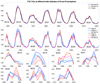 |
Fig. 1. Yearly hemispheric radio fluxes calculated at different helio-latitude intervals in 1948–2021. Top panel: all-hemispheric means of radio fluxes for the northern (N; blue line) and southern (S; red line) hemisphere in each year, together with the yearly mean radio flux (black line). Second panel: high-latitude (High), second high-latitude (2 High), and all-hemispheric radio fluxes for the northern (blueish colors) and southern (reddish colors) hemisphere. The seven small plots on the third and bottom row depict an enlarged view of the second panel, one for each of the seven solar cycle maxima. All fluxes are given in units of sfu. |
The second panel of Fig. 1 depicts radio fluxes for all three hemispheric heliolatitude (high-latitude, second high-latitude, and all-hemispheric) intervals. The largest differences between the northern and southern fluxes in the second panel of Fig. 1 are much larger in every cycle than the differences between the two all-hemispheric fluxes depicted in the top panel of Fig. 1. In most cycles, the highest value of the cycle is formed by one of the two (N or S) high-latitude fluxes, while the (nearly) simultaneous high-latitude flux of the opposite hemisphere often has the lowest value. As the high-latitude (and second high-latitude) fluxes are measured at higher (northern or southern) heliographic latitudes than the all-hemispheric fluxes, the differences between the northern and southern fluxes are seen to increase with increasing heliographic latitude. This also verifies that these differences are related to systematic spatial differences between the solar hemispheres and not to temporal variations.
Figure 1 shows that, for some cycles, the hemisphere with the largest radio flux is different for all-hemispheric fluxes (top panel) and high-latitude fluxes (second panel). This is the case, for example, for cycle 22, where the northern all-hemispheric fluxes form the peak in 1989 (top panel), while the southern high-latitude fluxes form the cycle maximum in 1991 (second panel). Furthermore, the second panel of Fig. 1 shows an interesting, systematic alternation, with northern heliolatitude fluxes forming cycle maxima in all three odd cycles (19, 21, 23) and southern heliolatitude fluxes forming cycle maxima in all four even cycles (18, 20, 22, 24). Using binomial statistics, one can estimate that such a systematic variation would occur randomly at the probability of less than 2%. This suggests that there is a systematic 22 yr oscillation in hemispheric 10.7 cm radio fluxes, which has so far remained unnoticed.
4. Fluxes around solar maxima
The alternation of cycle maximum fluxes between the two hemispheres from cycle to cycle is most clearly depicted in the enlarged plots of the two bottom rows of Fig. 1. The northern high-latitude flux is larger than all southern fluxes during the odd cycles, while the southern high-latitude flux is larger than all northern fluxes during the even cycles. We refer to the hemisphere with the cycle flux maximum as the dominant hemisphere during the respective cycle and to the opposite hemisphere as the recessive hemisphere (during that cycle).
During six cycle maxima (cycles 18–23), the largest flux is formed by the (either northern or southern) high-latitude flux of the dominant hemisphere. Only in one cycle (cycle 24) is the southern second high-latitude flux slightly higher than the southern high-latitude flux. At each cycle maximum, the high-latitude and second high-latitude fluxes of the dominant hemisphere are larger than all three simultaneous (half a year before or after) fluxes of the opposite (recessive) hemisphere. In five cycles (19–22, 24) out of seven, even the all-hemispheric flux of the dominant hemisphere is larger than all three simultaneous fluxes of the recessive hemisphere. In five cycles (18, 20–23), the three fluxes of the dominant hemisphere systematically increase with heliographic latitude (with the high-latitude flux being the largest and the all-hemispheric the smallest).
On the other hand, when studying the simultaneous fluxes of the recessive hemisphere (either of the two fluxes half a year away from the maximum of the dominant hemisphere), we find that the high-latitude flux is the smallest flux in four cycles, while the second high-latitude flux is smallest in cycle 18, and the all-hemispheric flux is smallest in cycles 21 and 22. Accordingly, at the same time as the heliolatitude fluxes of the dominant hemisphere are above the average and increase with heliolatitude, the heliolatitude fluxes of the opposite (recessive) hemisphere are below the average and, in most cycles, decrease with heliolatitude.
These results show that the cycle maximum fluxes are typically ordered with (signed) heliographic latitude. This ordering is especially clear in the dominant hemisphere of all cycles but is also very clear (in reverse order) in the recessive hemisphere in most cycles. This ordering is created by the fact that almost all sources of radio emissions (sunspots and non-sunspot active regions) are located at higher (northern or southern) latitudes than those reached by the Earth (±7.2°) during its yearly excursion. When the Earth’s heliolatitude increases either to the north or to the south, the contribution of the corresponding regions to radio flux increases and the contribution from the opposite hemisphere decreases. During those few cases when radio fluxes at cycle maxima did not follow a strict dependence on heliolatitude, some temporary activities must have occurred during the longer time interval (as in the six-month all-hemispheric interval) but outside the shorter (high-latitude) interval, changing the order of fluxes. As described above, such a change happened only once in the dominant hemisphere in cycle 24 between the high-latitude and second high-latitude interval.
5. High-latitude asymmetries at cycle maxima
We calculated the difference between the cycle maximum high-latitude radio flux (in the dominant hemisphere) and the larger of the two high-latitude fluxes in the recessive hemisphere within half a year from the cycle maximum. This difference is an appropriate measure of the asymmetry of high-latitude fluxes in each solar cycle (this definition leads to somewhat smaller asymmetries than perhaps the more symmetric alternative of using the mean of the two fluxes of the recessive hemisphere). We depict the corresponding (absolute) asymmetries for each cycle in the left plot of Fig. 2. The highest solar cycle 19 has the largest asymmetry of about 45 sfu, and the second highest cycle 22 has the second largest asymmetry of about 39 sfu. The mean value of the asymmetry over all cycles is about 30 sfu. The asymmetry of the lowest cycle 24, which is about 12 sfu, is much smaller than for any other cycle. Cycle 18 has the second smallest asymmetry of about 22 sfu. Omitting cycles 24 and 18, the mean asymmetry of cycles 19–23 is about 35 sfu. The corresponding standard deviation (std) is about 7 sfu, which means the std/mean ratio is 0.2.
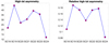 |
Fig. 2. Hemispheric difference (asymmetry) between cycle maximum high-latitude radio flux in the dominant hemisphere and the maximum high-latitude flux in the recessive hemisphere within half a year from the maximum. Left: absolute asymmetry (in units of sfu). Right: corresponding relative asymmetry obtained by normalizing the (absolute) asymmetry in the left plot by the mean of the two fluxes. |
The right plot of Fig. 2 depicts the corresponding relative asymmetry obtained by normalizing the asymmetry in the left plot of Fig. 2 by the mean of the two fluxes. The mean of the relative asymmetry over all seven cycles is about 0.15 and is about 0.17 over the five cycles 19–23; the corresponding standard deviations are 0.040 and 0.017. Accordingly, the (relative) asymmetry in the high-latitude radio flux between the dominant and recessive hemisphere is about 15 ± 4% for all cycles and about 17 ± 1% for the high cycles 19–23.
We also note that the standard deviation/mean ratio for the relative asymmetry of cycles 19–23 is only 0.1, which is roughly half of that for the (absolute) asymmetry. This reduction is another demonstration of the correlation between asymmetry and cycle height. Normalizing the asymmetry by the mean flux almost completely removes this correlation. Cycle 21 seems to have a somewhat smaller asymmetry than expected from its height. Even though cycle 24 is lower than other cycles, its relative asymmetry of about 0.082 remains very small even after normalization, making cycle 24 an outlier, which deviates from the five other cycles by 5 std. We also note that, according to the relative asymmetry, cycle 18 also considerably differs (by more than 3 std) from the other cycles. These results reveal an interesting temporal evolution of the (relative) asymmetry during the last seven solar cycles.
6. Flux-value distributions
Figure 3 depicts the daily high-latitude radio flux values in the northern (blue stars) and southern (red stars) hemisphere during 2 yr around the cycle maxima in descending rank order separately for each of the seven solar cycles. The panels of the left column show the distribution of flux values in the four even cycles, where the southern flux values are systematically above the northern fluxes. The opposite ordering is true for the three odd cycles depicted in the panels of the right column. The mean difference between the ranked fluxes is largest in cycle 19 and smallest in cycle 24, as expected from Figs. 1 and 2.
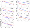 |
Fig. 3. Daily high-latitude radio flux values (in units of sfu) of the northern (blue stars) and southern (red stars) hemisphere during 2 yr around cycle maxima, in descending rank order, separately for each of the seven solar cycles (even cycles on left, odd cycles on right). |
We used the two-sided Wilcoxon rank sum test in order to test whether or not, in each solar cycle separately, the daily northern and southern fluxes are samples from the same distributions with equal medians. The Wilcoxon rank sum test (equivalent to Mann-Whitney U-test) is a nonparametric test, and has the additional advantage that the two populations can have different lengths, which is of use here as the northern high-latitude sections (70 days) are slightly longer than the southern (66 days) ones because of the eccentricity of the Earth’s orbit.
Using the 99% confidence limit in the test, we find that, for each cycle, the medians (and thereby the populations) are significantly different, with p-values (probability that the two populations are the same) varying from 2.9 × 10⁻¹⁷ (extremely improbable) for cycle 19 to 8.2 × 10⁻⁴ for cycle 24 (quite improbable). All p-values and the related years are given in Table 1. Accordingly, the Wilcoxon rank sum test verifies that the differences between the high-latitude fluxes of the dominant and recessive hemispheres around cycle maxima are significant, and that the corresponding flux populations (distributions) are different. This indicates, for example, that the differences between the radio fluxes of the dominant and recessive hemispheres, and thereby the corresponding hemispheric asymmetries, are not due to a small number of extreme events, such as large flares, causing a few exceptional radio flux values, but rather to a systematic difference between the radio flux distributions around cycle maxima.
Wilcoxon rank sum tests between 2 yr sections of northern and southern high-latitude radio fluxes, performed for each of the seven solar cycles.
7. Hale cycle in both hemispheres
Here, we study the continuous, long-term evolution of the three (high-latitude, second high-latitude, and all-hemispheric) radio fluxes separately in the northern and southern hemisphere. As radio fluxes show a large solar cycle variation, we normalize each of the three hemispheric fluxes of the two hemispheres by the annual (more precisely, 365 day, not calendar year) mean around the respective highest latitude time (March 6 for south and September 7 for north). This normalizes the radio fluxes from the different phases of solar cycle to the same level around unity, allowing a consistent long-term comparison.
The top panel of Fig. 4 shows the normalized northern and southern radio fluxes using the high-latitude (blue for N, red for S), second high-latitude (light blue for N, orange for S), and all-hemispheric (cyan for N, magenta for S) time intervals (colors are the same as in the second panel of Fig. 1). Although the variation of these hemispheric fluxes from year to year is relatively large, one can see that there are a number of time intervals when the northern fluxes (blueish colors) and southern fluxes (reddish colors) are on opposite sides of unity. This is the case, for example, around 1960, when the northern (southern) fluxes are larger (smaller) than unity, and in the early 1990s when the southern (northern) fluxes are larger (smaller) than unity. As expected, the largest, oppositely oriented values of the northern and southern fluxes during these intervals are best seen in the high-latitude fluxes.
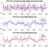 |
Fig. 4. Normalized hemispheric radio fluxes (in relative units). Top: normalized radio fluxes for the northern and southern hemisphere using high-latitude (blue for N, red for S), second high-latitude (light blue for N, orange for S), and all-hemispheric (cyan for N, magenta for S) time intervals (colors are the same as in the second panel of Fig. 1). Middle panel: yearly (thin blue) and 3 yr smoothed (thick blue) values of the normalized high-latitude radio flux for the northern hemisphere. A best-fit model consisting of two Fourier components is included as a black line. Bottom panel: same as in middle panel for the southern hemisphere, with blue color changed for red. |
The middle panel of Fig. 4 repeats the normalized northern high-latitude flux of the top panel as a thin blue line. Similarly, in the bottom panel of Fig. 4, we have reproduced the normalized southern high-latitude flux as a thin red line. In both panels, we include a 3 yr (three-point) smoothed (running mean) line of the corresponding yearly high-latitude flux. The smoothed line alleviates the large variability of the yearly values especially in the southern hemisphere (bottom panel of Fig. 4), making the long-term variation more visible. Both the northern and southern flux depict periods of a few years alternately above and below unity, indicating long-term oscillations.
In order to study this oscillation in more detail, we first found the dominant period of the long-term variation of fluxes by fitting the northern and southern smoothed fluxes separately with a harmonic function (one-harmonic model). We find that the dominant long-term oscillation is very close to the Hale cycle in both hemispheres, with the best-fit period being 20.7 yr in the north and 22.8 yr in the south. The corresponding amplitudes are 0.045 and 0.042.
However, it is evident from Fig. 4 that the variation of the normalized radio fluxes does not follow a pure (one-harmonic) sinusoid. Rather, the dominant Hale cycle seems to be modulated by a longer-term variation. In order to take into account this modulation, we used a model consisting of two Fourier components, the fundamental and the second harmonic, and fitted this two-harmonic model separately to the northern and southern normalized fluxes.
The middle and bottom panels of Fig. 4 include the corresponding best-fit results of the two-harmonic model as a black line. We find that, in both hemispheres, the second harmonic has a period close to the Hale cycle and is much stronger than the fundamental harmonic of the model. In the north (middle panel of Fig. 4), the Hale cycle period of the two-harmonic model is 20.8 yr, which is almost the same as in the one-harmonic model (the fundamental has, naturally, a period of twice this length). The power of the Hale cycle in the north is about three times the power of the fundamental. The two-harmonic model explains a considerable amount (almost 40%; r = 0.62) of the variation of the northern radio flux, and the correlation between the model and observations is highly significant (p < 2 × 10⁻⁸).
In the southern hemisphere (bottom panel of Fig. 4), the second harmonic is also the dominant Fourier component and has a period of 23.9 yr, which is close to the Hale period. The power of the Hale period in the south is almost twice that of the fundamental. Therefore, the fundamental harmonic (a long-period wave) modulates the Hale cycle more in the south than in the north, which is in agreement with a slightly smaller one-harmonic Hale cycle amplitude in the south than in the north. As in the north, the two-harmonic model explains a fair amount (almost one third; r = 0.56) of the low-frequency variation of the southern radio flux, and the correlation between the model and observations is very significant (p < 5 × 10⁻⁷). We also find a very significant negative correlation between the northern and southern fluxes (r = −0.52, p < 4 × 10⁻⁶).
As seen in the middle panel of Fig. 4, the normalized high-latitude radio fluxes of the northern hemisphere have maxima (minima) around the maxima of odd (even) cycles. On the other hand, the southern fluxes (see bottom panel of Fig. 4) have maxima (minima) around the maxima of even (odd) cycles, which is roughly opposite to the northern flux. These results are in excellent agreement with the above found relation between the hemispheric asymmetry of cycle peaks and the Hale cycle (see Fig. 1).
Finally, we note that there is considerable power in the normalized high-latitude radio fluxes of both hemispheres at higher frequencies, which is not explained by the long-period harmonics studied here. The strongest high-frequency harmonic is the sixth harmonic, which has a period of about 7 yr in the north and 8 yr in the south. This period is fairly close to the 8.6 yr periodicity, which was found in sunspot area asymmetry by Ballester et al. (2005) and was reproduced by Schüssler & Cameron (2018) in a dynamo simulation of hemispheric asymmetry. Finding these close-by periodicities in completely different datasets with very different analysis methods suggests that there is likely to be some physical cause behind this periodicity. This will be studied in more detail in a separate publication.
8. High-latitude sunspot numbers
The finding of systematic hemispheric asymmetries in solar radio flux at the level of about 15%–17% around cycle maxima and about 4%–5% over the whole cycle depicts a considerably larger variability than the estimated error for the 10.7 cm radio flux of about 1% (Tapping 2013). Therefore, it is very unlikely that the observed asymmetry pattern is due to measurement errors. As we discuss above, it is also extremely unlikely that this systematic pattern arises from random fluctuations in radio flux. Therefore, as the solar radio flux is known to be a close proxy of solar activity, we may expect the observed pattern to reflect a real hemispheric asymmetry in the emergence of solar magnetic flux, and should be seen in other related proxies of solar activity as well.
It is known that at least 60% of the activity-dependent F10.7 flux is in the form of bremsstrahlung emission from non-sunspot active regions (typically plages), while less than 10% of radio flux comes from sunspots (Schonfeld et al. 2015). However, as the occurrence of plages follows the sunspot occurrence (sunspot cycle) relatively closely, radio flux and sunspots also follow each other relatively closely, at least on monthly and longer timescales (Covington 1947; Lehany & Yabsley 1948; Johnson 2011; Tiwari & Kumar 2018; Clette 2021). Accordingly, the notable hemispheric asymmetries found here in solar radio flux should also be visible in sunspots.
Figure 5 shows analogous plots for sunspot numbers as was presented in Fig. 1 for radio flux. The top panel of Fig. 5 depicts the mean sunspot numbers during the northern and southern all-hemispheric intervals in each year from 1948 to 2021, together with the corresponding yearly mean sunspot numbers. As for the corresponding plot of radio fluxes (top panel of Fig. 1), the top panel of Fig. 5 shows some small differences between the northern and southern all-hemispheric sunspot numbers, mostly around solar maxima. The relative hemispheric differences are fairly similar for sunspot numbers and radio flux, but the dominant hemisphere is not always the same for the all-hemispheric fluxes of these two parameters.
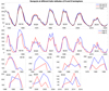 |
Fig. 5. Yearly hemiSSNs calculated at different helio-latitude intervals in 1948–2021. Top panel: all-hemispheric means of daily sunspot numbers for the northern (all-hemi N; blue line) and southern (all-hemi S; red line) hemisphere, together with the yearly mean sunspot numbers (black line). Second panel: high-latitude sunspot numbers for the northern (High N) and southern hemisphere (High S). The seven small plots on the third and bottom rows depict an enlarged view of the second panel, for each of the seven solar cycle maxima. |
The second panel of Fig. 5 depicts sunspot numbers for the high-latitude intervals of the northern and southern hemisphere (for clarity, we omit the second high-latitude and all-hemispheric sunspot numbers). There is dramatic overall agreement between the hemispheric high-latitude sunspot numbers (second panel of Fig. 5) and hemispheric high-latitude radio fluxes (red and blue lines in the second panel of Fig. 1). The temporal variations of the high-latitude sunspot numbers and high-latitude radio fluxes follow each other quite closely in both hemispheres, although some differences can be seen in some cycles. For example, the northern dominance in cycles 21 and 23 is more systematic in high-latitude sunspot numbers than radio flux, while the southern dominance in cycle 22 is somewhat more clear in high-latitude radio flux than in sunspot numbers.
Most interestingly, the hemispheric high-latitude sunspot numbers and radio fluxes depict the same pattern of alternating hemispheric dominance at cycle maxima, with high-latitude sunspot numbers (and radio flux) of the northern hemisphere forming cycle maxima during all odd cycles and sunspot numbers (and radio flux) of the southern hemisphere dominating during all even cycles.
9. Sunspot number asymmetry
Figure 6 shows the absolute (left panel) and relative (right panel) hemispheric asymmetry between dominant and recessive high-latitude sunspot numbers, with sunspot number asymmetry defined analogously to radio flux asymmetry, which is repeated here from Fig. 2 for a comparison of sunspot and radio flux asymmetries. We note that both the absolute and the relative asymmetries are considerably larger for sunspot numbers than for radio fluxes in all cycles, except for cycles 18 and 22. The mean absolute sunspot asymmetry of all cycles is 46, and is 57 for cycles 19–23, both approximately 50% larger than for radio flux. As for radio flux, cycle 19 has the largest absolute sunspot number asymmetry but, contrary to radio flux, cycle 24 has only the third smallest asymmetry.
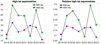 |
Fig. 6. Hemispheric asymmetries between dominant and recessive high-latitude sunspot numbers (black line with green circles) and radio fluxes (blue line with red squares (repeated from Fig. 2). Left: absolute asymmetries. Right: corresponding relative asymmetries obtained by normalizing the (absolute) asymmetries in the left plot by the mean of the two sunspot numbers/fluxes. |
The mean relative asymmetry for sunspot numbers over all seven cycles is about 0.23 and is about 0.27 over the five cycles 19–23. Thus, even the relative asymmetry is roughly 50% larger for sunspot numbers than for radio flux. The standard deviations in the two cases are 0.12 and 0.11 (these are almost the same, because cycle 22, which causes much of variance, is included in both cases). Accordingly, the relative asymmetry in the high-latitude sunspot numbers between the dominant and recessive hemisphere is about 23 ± 12% for all cycles and about 27 ± 11% for the high cycles 19–23.
10. Hemispheric sunspot numbers
Let us now study the hemiSSNs that are available at SILSO. These were produced at the same time and using the same method as the total (international) sunspot number since 1992. The sum of the two hemiSSNs yields the total sunspot number. Accordingly, these numbers can be considered as the most reliable version of any hemispheric sunspot numbers. The left plot of Fig. 7 presents the yearly means of daily hemiSSNs in 1992–2022 for the northern (N) and southern (S) hemisphere. The maximum yearly hemispheric sunspot activity during cycle 24 was recorded in 2014 in the southern hemisphere, which in agreement with the view obtained from the high-latitude vantage point (see Fig. 5). However, the highest yearly hemiSSN during cycle 23 was obtained in 2002 in the southern hemisphere, while the northern peak in 2001 remains a couple of units lower. This is in contrast to the view obtained from the high-latitude sunspot numbers depicted in Fig. 5 and suggests that the high-latitude sunspot numbers and yearly hemiSSNs do not always yield exactly the same view on hemispheric differences. We also note that the sum of yearly means of hemiSSNs remains far below 200 in each year of cycle 23, while the maximum high-latitude sunspot number is above 200 (see Fig. 5).
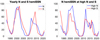 |
Fig. 7. Hemispheric sunspot numbers. Left: yearly means of daily hemiSSNs for the northern (N) and southern (S) hemisphere. Right: northern hemiSSNs observed at high heliographic northern (high N) and southern (high S) latitudes. |
The right plot of Fig. 7 depicts the northern hemiSSNs observed at the northern (N) and southern (S) high-latitude vantage points. It is important to note how different the time evolution of the northern hemiSSNs is between the N and S high-latitude vantage points. During cycle 23, the northern hemiSSNs are consistently larger in the northern vantage point than in the southern one, in every year from 1997 to 2005. This difference is largest in 2001, which is the maximum year for both the yearly northern sunspot numbers (left plot of Fig. 7) and for the total sunspot number viewed from the northern vantage point (see Fig. 5). This consistent dominance of the northern vantage point indicates that a considerable fraction of sunspots of the northern hemisphere are not seen at the southern vantage point. Therefore, the northern hemiSSNs are underestimated at the (time of the) southern vantage point, that is, in spring time.
Moreover, the monthly means of northern hemiSSNs during the three spring months from February to April (not shown here) are systematically below the three fall months in the same years, namely 1997-2005, in analogy to the right plot of Fig. 7. This implies that the yearly northern hemiSSNs are considerably underestimated. Taking into account that the maximum of the northern hemispheric numbers in 2001 is only slightly below the southern peak in 2002, it is very likely that a correct value of northern hemiSSNs (obtained when viewed from an unbiased vantage point) would reveal the maximum of cycle 23 to be in the northern hemisphere in 2001, as depicted in Fig. 5. We did not find a similar underestimation of southern hemispheric numbers when viewed from the north. On the contrary, the southern hemiSSNs in three consecutive years from 2001 to 2003 are considerably larger (on average by some 30) when viewed from the north than when viewed from the south. Even in the maximum year, 2002, the southern sunspot numbers are more than 20 larger when viewed from the north than when viewed from the south. Currently, we do not know what could cause this obvious underestimation of hemiSSNs when viewed from the south (i.e., around the high heliolatitude time in spring); a detailed study of hemiSSNs is needed to answer this question.
11. Discussion
Here, we present a study of the 10.7 cm solar radio flux using the NOAA F10.7 index in 1947–2018 and continued thereafter by the Penticton noon flux values. We calculated radio fluxes at three different time intervals of increasing (absolute) heliographic latitude in order to create radio fluxes that increasingly weight emissions from one of the two hemispheres. We find that the hemispheric differences at cycle maxima increase (decrease) with increasing absolute heliographic latitude in the dominant (recessive) hemisphere and that fluxes calculated above 6° of (N or S) heliographic latitude, alternate systematically so that the northern hemisphere dominates during all odd cycles (19, 21, 23) and the southern hemisphere dominates during all even cycles (18, 20, 22, 24).
We also find that the mean relative hemispheric asymmetry, as measured by the normalized difference between high-latitude radio fluxes in the dominant and recessive hemispheres at cycle maxima, is about 15 ± 4% for all cycles and about 17 ± 1% for the high cycles 19–23. The relative asymmetry increases from about 11% during cycle 18 to the maximum of about 19% during the highest cycle 19, remains somewhat smaller during cycles 20–23, and then decreases to the smallest asymmetry of about 8% during cycle 24. This temporal evolution of the observed hemispheric asymmetry has interesting implications.
We show that the differences between the mean hemispheric high-latitude radio fluxes are not due to the effect of randomly occurring days with extremely large fluxes (due, e.g., to large flares). Rather, the distributions of daily radio flux values around maxima in the dominant and in the recessive hemisphere are statistically different at a very high confidence level. The largest difference, with an extremely high significance (p = 2.9 × 10⁻¹⁷; see Table 1), is found for cycle 19 and the smallest difference, with the lowest significance (p = 8.2 × 10⁻⁴), is found for cycle 24. This gives additional support to the above finding that hemispheric asymmetry has declined, together with solar activity, from the very high cycle 19 to the much lower cycle 24.
Normalizing the radio fluxes against solar activity level using annual (365 days around high-latitude times) averages, we find that both the northern and southern high-latitude fluxes depict a significant oscillation, the period of which is close to the Hale cycle, and the amplitude of which is modulated by a longer-period variation. The northern and southern radio fluxes oscillate roughly in anti-phase and have a strong negative mutual correlation. The amplitude of the Hale cycle in the north is about 5% and in the south is about 4%. This oscillation forms a new type of 22 yr Hale cycle-related variation.
The results based on daily high-latitude sunspot numbers agree very well with the corresponding radio fluxes. Similarly to radio fluxes, the high-latitude hemispheric sunspot numbers alternate systematically from northern dominance during odd cycles to southern dominance during even cycles. This verifies that the emergence of new magnetic flux on the solar surface oscillates with the 22 yr (Hale-related) cycle between the two hemispheres.
The longest contiguous period of northern sunspot dominance, which occurred during cycle 19 and part of cycle 20, has long been known (Swinson et al. 1986; Temmer et al. 2006). Northern dominance in yearly (or 13-month smoothed) sunspots started in 1958, while we find here that the northern dominance already started a couple of years earlier both in high-latitude radio fluxes (see the second small panel of Fig. 1) and in high-latitude sunspot numbers (see the second small panel of Fig. 5). Northern dominance in yearly sunspots lasted until 1971, beyond the maximum of cycle 20, while the hemispheric asymmetry in high-latitude radio fluxes and sunspot numbers had reversed to southern dominance already several years earlier (see the third small panel of Figs. 1 and 5).
Radio fluxes (and total sunspot numbers) measured at high heliolatitudes are clearly not purely hemispheric fluxes (numbers) but contain emissions (numbers) from both solar hemispheres. Accordingly, yearly means of hemiSSNs, for example, may not depict exactly the same hemispheric asymmetry as the high-latitude hemispheric means. We compared hemispheric and high-latitude sunspot numbers during cycles 23 and 24, and argue that the (rather small) difference in cycle 23 in fact reflects an inconsistency in hemispheric sunspots, which underestimates the northern sunspot numbers when viewed from the southern high-latitude vantage point.
The results presented here are novel, but have connections to some earlier Hale-cycle-related observations. Swinson et al. (1986) found a 22 yr periodicity in the normalized hemispheric asymmetry of sunspots. In previous investigations, we found (Zieger & Mursula 1998; Mursula & Zieger 2001; Mursula et al. 2002) that the average solar wind speed at 1 AU is faster (slower) in spring (i.e., at high southern heliolatitudes) than in fall in the late declining to minimum phase of even (odd) cycles. This indicates a systematic 22 yr oscillation of the mean latitude of the streamer belt. Stronger radio flux and larger sunspot numbers in the south in even maxima suggest stronger magnetic fields emerging on the solar surface, which then form stronger magnetic flux surges to the southern pole than to the north. Stronger surges in the south during the declining phase of even cycles create larger polar coronal holes, with larger extensions to southern low latitudes. Larger extensions produce more fast solar wind streams at southern heliographic latitudes, which is in agreement with earlier findings. Therefore, the phasing of the Hale cycle in radio waves agrees with the earlier-found phasing of the shifted streamer belt.
The generation of solar magnetic fields can be understood in terms of the action of a solar dynamo mechanism operating in the solar convection layer (for a review see, e.g., Dikpati & Gilman 2009; Dikpati 2016; Cameron et al. 2017; Brun & Browning 2017; Charbonneau 2020). Although dynamo models can explain many observational facts on solar activity and solar cycles, they cannot explain possible systematic patterns in the long-term (multi-cycle) variation in the height (or intensity) or asymmetry of solar cycles. The variability in poloidal to toroidal conversion (Ω mechanism) is relatively small, which allows, for example, a fairly accurate prediction of cycle maxima based on previous minimum-time polar fields. However, there is much more variability in toroidal to poloidal conversion (α mechanism), because of the greater stochasticity in related processes (meridional transport, possible non-Hale and/or non-Joy sunspots, etc.), which seriously limits the predictability of cycle properties beyond the next cycle (see, e.g., Muñoz-Jaramillo et al. 2013).
11.1. Relic field
One systematic long-term pattern is the pairing of cycles to even–odd pairs consisting of a lower (or less intense) even cycle and a higher (or more intense) odd cycle, the so-called Gnevyshev-Ohl (G-O) rule 1948, and the related 22 yr variation in sunspot activity (Mursula et al. 2001). Relic magnetic fields (and related electric currents) sustained in the Sun since the formation of the Solar System have been proposed to explain the G-O rule (Levy & Boyer 1982; Sonett 1983; Boyer & Levy 1984; Mursula et al. 2001). For example, relic electric currents flowing at the bottom of the convection layer in the direction of solar rotation would produce relic magnetic fields that enhance poleward oriented dynamo fields during a positive-polarity minimum and reduce them during a negative-polarity minimum. This would lead, via the conversion of poloidal to toroidal fields of the dynamo mechanism, to a higher-than-average odd cycle and a lower-than-average even field, explaining the G-O rule.
Even if a relic field exists at the bottom of the convection layer, the dynamo mechanism includes the same physical processes and these operate mostly in the same way as without the relic. The conversion of poloidal to toroidal field would proceed in the same way as without relic field, and would lead to enhanced and reduced hemispheric activities in the toroidal phase. As this modulation is only about 15%–20%, even at maximum, the relic field is considerably weaker than the dynamo field, at least during times of normal (or high) solar activity. We also note that the close phasing of the observed 22 yr cycle of hemispheric dominance with the Hale cycle of solar magnetic polarity reflects the important role of the dynamo conversion process in producing the observed Hale-cycle variation.
However, we note that the existence of a relic field makes the dynamo somewhat less vulnerable in the dominant hemisphere to the stochastic effects of the toroidal-to-poloidal conversion, because ensuing larger toroidal field would bias the probability distribution toward stronger poloidal field, increasing predictability. Roughly speaking, relic field raises the base level of the varying dynamo fields slightly higher in the dominant hemisphere, thereby affecting the probability distribution in favor of a higher cycle. On longer timescales, the centennial motion of the relic shift around the solar equator systematically modulates the effect of the relic, enhancing the possibility to predict solar activity over several cycles.
If the relic currents are located symmetrically around the solar equator, the relic field would enhance or reduce the fields statistically by equal amounts in the northern and southern hemisphere. Therefore, symmetrically located relic currents and fields cannot explain the current observations of systematic differences between the two solar hemispheres, nor their systematic alternation from cycle to cycle. However, if the distribution of relic currents is shifted slightly northward from the solar equator (keeping the relic field oriented northward), the relic field would, during a positive polarity minimum, enhance polar fields more strongly in the northern hemisphere than in the southern hemisphere, leading to the observed northern dominance in the subsequent odd cycle. Correspondingly, during a negative polarity minimum, it would reduce polar fields more strongly in the northern hemisphere than in the southern one, leading to the observed southern dominance in the subsequent even cycle.
We note that a northward oriented relic field would naturally prevail the observed phasing of the G-O rule (odd cycles higher than even cycles), irrespective of whether the shift is northward or southward (or no shift at all). However, a southward-shifted relic would lead to southern dominance in odd cycles and northern dominance in even cycles, which is opposite to current observations. On the other hand, if the relic currents were to flow in the opposite direction, that is, opposite to solar rotation, the relic field would enhance poleward fields during a negative polarity minimum and reduce them during a positive polarity minimum, leading to an opposite phasing of the G-O rule (higher even cycles). This would be the case, again, irrespective of a possible latitudinal shift of the relic. With this direction, a southward-shifted relic would agree with the observed hemispheric dominance, while a northward shift would violate it. In summary, the relic current orientation determines the phasing of the G-O rule (as found earlier), while the latitudinal shift of the relic determines the phasing of the alternating hemispheric dominance (as found here).
If the relic field is shifted northward, the northern field experiences a larger increase during odd cycles than the southern field during even cycles, and a larger reduction during even cycles than the southern field during odd cycles. Thus, both the northern and southern hemisphere experience a 22 yr variation with opposite phasing, but the 22 yr variation of northern hemisphere is of a larger amplitude than that of the southern hemisphere. These predictions are in good agreement with our observation (see Fig. 4) of a 22 yr oscillation in both hemisphere and a slightly stronger Hale cycle in the north than in the south. Accordingly, a northward-shifted relic field explains all the current observations, and also agrees with the phasing of the G-O rule.
We find that the hemispheric asymmetry in radio flux was largest (even when normalized by activity) during cycle 19, and was by far smallest during cycle 24. We suggest that this is due to the change of the relic shift from its widest northward shift during cycle 19 to zero or close to zero during cycle 24. Therefore, cycle 19 was one turning point of a long-term oscillation of a latitudinal shift of the relic, and the time interval between the two cycles, namely of about 50 yr, forms one-quarter of this oscillation. This suggests that the relic shift experiences an oscillation of about 200 yr. This is most likely the well-known 210 yr Suess/deVries cycle (Suess 1980; Sonett & Finney 1990; Ma & Vaquero 2020). The current results also provide an explanation for this cycle as the cycle made by the relic shift (relic average location) in the north–south direction. In previous investigations, we showed that the north–south asymmetry of the streamer belt experiences a long-term oscillation around the solar equator (Mursula & Zieger 2001; Mursula & Hiltula 2004), roughly at a 200 yr period. Accordingly, the streamer belt also oscillates at the same relic shift (Suess/deVries) cycle.
The fact that cycle 19 (cycle 24) marks the highest (smallest) solar cycle in the last 100 yr supports the idea that hemispheric asymmetry is an important factor in modulating long-term solar activity, and that a large (small) hemispheric asymmetry is connected with high (low) solar activity. A shifted relic field can naturally explain this connection. When the relic shift is large (and northward, as in the 20th century), the relic field enhances the dynamo poloidal fields very effectively in the dominant (northern) hemisphere, leading to high activity in that hemisphere. It also enhances the activity in the opposite (southern) hemisphere, although far less than in the dominant hemisphere, leading to a very large and highly asymmetric cycle, as seen for cycle 19. On the other hand, with little or no shift, the relic field affects both hemispheres only slightly and relatively equally, leading to a rather weak, fairly symmetric cycle. We also note that the height of cycle 24 is also reduced by the fact that relic and dynamo fields are opposite during the previous minimum, which makes cycle 24 to be unfavored by the G-O rule.
A sequence of high cycles is formed when the relic shift is large, which happens twice during the 210 yr oscillation, once northward (e.g., during the 20th century) and once southward (like that in the 19th century and in the ongoing 21st century). Accordingly, the relic shift oscillation also explains the long-term variation in the height of solar cycles, known as the Gleissberg cyclicity (Gleissberg 1939, 1958). Two successive Gleissberg cycles have opposite relic shifts and form one full relic field shift (asymmetry) cycle, in analogy to two successive 11 yr solar activity (Schwabe) cycles with opposite polarities forming one full 22 yr magnetic (Hale) cycle.
11.2. Multi-cycle forecast
The suggested explanation for the results presented here in terms of a relic field whose direction and amplitude remain constant but whose latitude is slowly oscillating offers a possibility to make some very long-term (multi-cycle) forecasting. The current lull in solar activity will be replaced with a reactivation as the relic shift starts increasing, now toward the southern hemisphere. During the ongoing cycle 25, the relic shift is expected to remain rather small, which reduces the growth of this cycle. However, the previous solar minimum around 2019 was positive, and relic and dynamo fields were aligned. Accordingly, cycle 25 is G-O rule favored, which will very likely increase its height to somewhat higher than cycle 24. Depending on the amount of shift, cycle 25 may already be dominated by southern hemispheric activity.
The orientation of the poloidal phase of the dynamo reverses to the next minimum, leading to an opposite orientation of the relic and dynamo fields (configuration unfavored by the G-O rule). This reduces the height of cycle 26, and it will remain rather low, perhaps even lower than cycle 25. As the relic is already expected to be shifted southward during cycle 26, the activity will quite likely be dominated by the northern hemisphere. We also note that the alternation of hemispheric activity in this century will be in opposite phase to that of the 20th century because of the opposite (southward) relic shift in the 21st century.
By the time of cycle 27, the relic shift is expected to be already quite large (relative to its final southward extent). Since cycle 27 is also G-O favored (relic and dynamo fields aligned during the previous minimum), it will be a relatively high cycle, considerably higher than cycle 26, possibly reaching the yearly sunspot level of 200. Also, due to the relic shift, the activity in cycle 27 will very likely be dominated by the southern hemisphere. Cycle 28 will also be fairly high but, as it is unfavored by the G-O rule, it will not be a record cycle, and may even remain lower than cycle 27. In line with the alternation of hemispheric dominance, cycle 28 will most likely be northern-dominated.
Most interestingly, according to our scenario, the relic shift will attain its largest southward extent during cycle 29. Therefore, we can forecast with considerable confidence that cycle 29 will be the highest of all five previous cycles (25-29), forming a highly active centennial maximum of the 21st century, in analogy to cycle 19, which was the record cycle of the 20th century. Cycle 29 will also be characterized by a record large dominance of the southern hemisphere.
Overall, during the 21st century, odd cycles tend to be higher and dominated by the southern hemisphere, while even cycles are lower and dominated by the northern hemisphere, in opposite phasing to the hemispheric order of the 20th century found here. After the centennial peak of cycle 29, the relic shift starts declining, leading to a period of about five cycles with cycle heights decreasing alternately, following the G-O rule.
The above forecasting is based on an ideal, unperturbed interpretation of the relic model. However, the dynamo mechanism will produce variability in the above predictions, mainly because of stochastic fluctuations during the toroidal-to-poloidal conversion, as noted above. It may be possible to estimate the probability of the above forecasts in the future, which would take this variability into account. One could construct an observation-based probability model for the interaction of relic and dynamo fields as a function of the shift, with dynamo fluctuations producing variations to be included as a model parameter. A slightly more physical model would be to locate relic currents at the bottom of the convection layer and calculate their effect on the dynamo field (again, as a function of the shift) and include this in a probability model. However, the most physical (and natural) method would be to include a shifted relic field in a dynamo model. Then, a series of dynamo runs for different shifts would yield the most realistic estimate of the distribution of cycle heights and asymmetries as a function of relic shift. We expect such modified dynamo models to be run in the near future.
12. Conclusions
In conclusion, here we used the daily solar F10.7 radio fluxes and daily sunspot numbers for the last 75 yr, as well as a novel method based on helio-latitudinally varying vantage points, to study the long-term evolution of solar hemispheric asymmetry. Our findings can be summarized as follows.
-
Cycle maxima of solar 10.7 cm radio fluxes increase with the heliolatitude of the vantage point in the dominant hemisphere (northern hemisphere in odd cycles, southern in even cycles), while simultaneous fluxes decrease in the recessive hemisphere (southern hemisphere in odd cycles, northern in even cycles). Accordingly, radio fluxes measured at increasingly high heliolatitudes include an increasing fraction from the corresponding hemisphere and therefore yield interesting information about hemispheric radio fluxes and their differences.
-
Cycle maxima of high-latitude radio fluxes are found in the northern hemisphere during all three odd solar cycles (19, 21, 23) and in the southern hemisphere during all four even cycles (18, 20, 22 24) covered by the 75 yr sequence of F10.7 observations. This alternation indicates a new form of systematic 22 yr (Hale-cycle-related) variation in solar radio fluxes.
-
The difference between the dominant and recessive hemisphere at cycle maxima is largest during cycle 19 and smallest in cycle 24, even when using normalized fluxes. Average radio flux asymmetry at cycle maxima is about 15 ± 4% for all cycles and about 17 ± 1% for the high cycles 19–23.
-
Normalizing the high-latitude radio fluxes by yearly means in order to study the asymmetry continuously throughout the solar cycle, we find that the normalized radio fluxes depict a dominant Hale cycle in both hemispheres, with opposite relative phase. The amplitude of the Hale cycle is about 5% in the northern hemisphere and about 4% in the south. These results explain the alternating hemispheric dominance at cycle peaks, and generalize the Hale cycle to high-latitude radio fluxes in both hemispheres.
-
Daily sunspot numbers depict the same ordering with heliolatitude and the same alternation of the dominant hemisphere, with larger sunspot numbers at cycle maxima in the northern hemisphere during odd cycles and in the southern hemisphere during even cycles. The mean hemispheric asymmetry in sunspot numbers (about 23% over all seven cycles and 27% over cycles 19–23) is roughly 50% larger than in radio flux. These results verify that the hemispheric differences and variations found in radio fluxes are due to similar properties in magnetic flux emergence.
-
Our results give additional support to the existence of relic magnetic fields in the Sun. A northward-oriented relic field (produced by currents flowing in the direction of solar rotation in the upper radiation or lower convection zone) has previously been proposed to explain the long-held G-O rule of cycle pairing to lower even cycles and higher odd cycles. Relic fields can enhance (reduce) poleward dynamo fields that have the same northward (opposite southward) polarity as the relic field. However, a relic field located symmetrically around the solar equator cannot explain systematic differences in the two hemispheres.
-
A relic field can explain the observed hemispheric Hale cycle if it is shifted slightly northward. Accordingly, in the odd cycles, the northern hemisphere will be enhanced more than the southern hemisphere and, in the even cycles, the northern hemisphere will be reduced more than the southern hemisphere. This leads to a Hale-cycle-related alternation of hemispheric asymmetry and also to anti-phased Hale cycles in both hemispheres.
-
We interpret the temporal change of hemispheric asymmetry from the highly asymmetric cycle 19 to very weakly asymmetric cycle 24 in terms of a decrease in the relic shift from its maximum in cycle 19 to almost zero in cycle 24. This implies that the relic shift oscillates one full cycle around the solar equator during the 210 yr Suess/deVries period. This also explains the physical cause of this periodicity. The drop in hemispheric asymmetry from cycle 19 to cycle 24 forms one-quarter of this oscillation. This oscillation also explains the previously found roughly 200 yr oscillation in the heliolatitude location of the streamer belt, in the related hemispheric asymmetry of solar wind, and in the phase of the annual variation in geomagnetic activity (Mursula & Zieger 2001; Mursula & Hiltula 2004).
-
Large hemispheric asymmetry and high solar activity occur at the same time because they are both produced at the time when the relic field is shifted away from solar equator. During the 20th century, the relic made one northward excursion from the equator and back, which formed one high Gleissberg cycle. Accordingly, Gleissberg cycles are explained as one half of the relic-shift oscillation cycle, that is, the Suess/deVries cycle. Northern dominance was strongest during cycle 19, which was also the highest cycle in the 20th century and the turning point of the relic-shift oscillation.
-
This interpretation allows very long-term forecasting of solar activity. We expect cycle 25 to remain only slightly larger than cycle 24, because the shift is still relatively small. Cycle 25 is probably south-dominated. Also, cycle 26 will remain rather small because it is unfavored by the G-O rule. Cycle 26 is quite likely north-dominated. Cycle 27 will be much higher than the three preceding cycles, probably reaching 200 in yearly numbers, because the shift is already relatively large (in relation to its maximum extent) and the relic orientation is favorable (this cycle is favored by the G-O rule). Cycle 27 is very likely south-dominated. Cycle 28 will also be quite high and north-dominated, but may remain even lower than cycle 27. Finally, cycle 29 will be the century-high cycle, an analog of cycle 19 in the 21st century. It will also be marked by strong dominance of activity in the southern hemisphere. These forecasts are based on an unperturbed interpretation of the relic model. As discussed above, the dynamo mechanism will produce variability in these predictions due to stochastic fluctuations during the toroidal-to-poloidal conversion. The effect of this variability can be estimated using dynamo models including the relic field, leading to forecasts with more accurate probability estimates with errors.
Our observations open up a new direction in space climate research, including studies of long-term solar activity, solar magnetism, solar magnetic field (dynamo) modeling, and long-term solar wind and solar-terrestrial environment. The proposed scenario in terms of a shifted relic field not only provides an explanation for hemispheric asymmetries but also emphasizes their importance for solar activity and its significance as a signature of solar internal processes.
Acknowledgments
We dedicate this paper to Ken Tapping and other long-term observers of solar radio flux in Canada. We acknowledge the Lisird server (https://lasp.colorado.edu/lisird/) for providing a link to the NOAA F10.7 cm index. The recent Penticton 10.7 cm data were retrieved from the NRCan server (https://www.spaceweather.gc.ca/forecast-prevision/solar-solaire/solarflux/sx-5-flux-en.php), which is served by the Solar Radio Monitoring Program operated jointly by the National Research Council Canada and Natural Resources Canada with support from the Canadian Space Agency. We acknowledge the service of daily total and hemispheric sunspot data (version 2) at the World Data Center SILSO, Royal Observatory of Belgium, Brussels (SILSO World Data Center 1947-2022).
References
- Antonucci, E., Hoeksema, J. T., & Scherrer, P. H. 1990, ApJ, 360, 296 [Google Scholar]
- Ballester, J. L., Oliver, R., & Carbonell, M. 2005, A&A, 431, L5 [NASA ADS] [CrossRef] [EDP Sciences] [Google Scholar]
- Bhowmik, P. 2019, A&A, 632, A117 [NASA ADS] [CrossRef] [EDP Sciences] [Google Scholar]
- Boyer, D. W., & Levy, E. H. 1984, ApJ, 277, 848 [NASA ADS] [CrossRef] [Google Scholar]
- Brun, A. S., & Browning, M. K. 2017, Liv. Rev. Sol. Phys., 14, 4 [Google Scholar]
- Cameron, R. H., Dikpati, M., & Brandenburg, A. 2017, Space Sci. Rev., 210, 367 [Google Scholar]
- Carbonell, M., Oliver, R., & Ballester, J. L. 1993, A&A, 274, 497 [NASA ADS] [Google Scholar]
- Charbonneau, P. 2020, Liv. Rev. Sol. Phys., 17, 4 [Google Scholar]
- Clette, F. 2021, J. Space Weather Space Clim., 11, 2 [NASA ADS] [CrossRef] [EDP Sciences] [Google Scholar]
- Clette, F., Svalgaard, L., Vaquero, J. M., & Cliver, E. W. 2014, Space Sci. Rev., 186, 35 [CrossRef] [Google Scholar]
- Clette, F., Cliver, E. W., Lefèvre, L., Svalgaard, L., & Vaquero, J. M. 2015, Space Weather, 13, 529 [NASA ADS] [CrossRef] [Google Scholar]
- Clette, F., Cliver, E. W., Lefèvre, L., et al. 2016, Sol. Phys., 291, 2479 [NASA ADS] [CrossRef] [Google Scholar]
- Covington, A. E. 1947, Nature, 159, 405 [CrossRef] [Google Scholar]
- Dikpati, M. 2016, Asian J. Phys., 25, 341 [Google Scholar]
- Dikpati, M., & Gilman, P. A. 2009, Space Sci. Rev., 144, 67 [NASA ADS] [CrossRef] [Google Scholar]
- Duchlev, P. I. 2001, Sol. Phys., 199, 211 [NASA ADS] [CrossRef] [Google Scholar]
- Garcia, H. A. 1990, Sol. Phys., 127, 185 [NASA ADS] [CrossRef] [Google Scholar]
- Gleissberg, W. 1939, The Observatory, 62, 158 [NASA ADS] [Google Scholar]
- Gleissberg, W. 1958, J. Br. Astron. Assoc., 68, 148 [Google Scholar]
- Gnevyshev, M. N., & Ohl, A. I. 1948, Astron. Zh., 25, 18 [Google Scholar]
- Hiltula, T., & Mursula, K. 2006, Geophys. Res. Lett., 33, L03105 [NASA ADS] [CrossRef] [Google Scholar]
- Johnson, R. W. 2011, Astrophys. Space Sci., 332, 73 [NASA ADS] [CrossRef] [Google Scholar]
- Kitchatinov, L., & Khlystova, A. 2021, ApJ, 919, 36 [NASA ADS] [CrossRef] [Google Scholar]
- Knaack, R., Stenflo, J. O., & Berdyugina, S. V. 2004, A&A, 418, L17 [NASA ADS] [CrossRef] [EDP Sciences] [Google Scholar]
- Knaack, R., Stenflo, J. O., & Berdyugina, S. V. 2005, A&A, 438, 1067 [CrossRef] [EDP Sciences] [Google Scholar]
- Krueger, A. 1979, Geophys. Astrophys. Monogr., 16, 23 [NASA ADS] [Google Scholar]
- Lehany, F. J., & Yabsley, D. E. 1948, Nature, 161, 645 [NASA ADS] [CrossRef] [Google Scholar]
- Levy, E. H., & Boyer, D. 1982, ApJ, 254, L19 [NASA ADS] [CrossRef] [Google Scholar]
- Ma, L., & Vaquero, J. M. 2020, Open Astron., 29, 28 [NASA ADS] [CrossRef] [Google Scholar]
- Muñoz-Jaramillo, A., Dasi-Espuig, M., Balmaceda, L. A., & DeLuca, E. E. 2013, ApJ, 767, L25 [CrossRef] [Google Scholar]
- Mursula, K. 2007, Adv. Space Res., 40, 1034 [NASA ADS] [CrossRef] [Google Scholar]
- Mursula, K., & Hiltula, T. 2003, Geophys. Res. Lett., 30, 2135 [NASA ADS] [CrossRef] [Google Scholar]
- Mursula, K., & Hiltula, T. 2004, Sol. Phys., 224, 133 [Google Scholar]
- Mursula, K., & Zieger, B. 2001, Geophys. Res. Lett., 28, 95 [NASA ADS] [CrossRef] [Google Scholar]
- Mursula, K., Usoskin, I. G., & Kovaltsov, G. A. 2001, Sol. Phys., 198, 51 [NASA ADS] [CrossRef] [Google Scholar]
- Mursula, K., Hiltula, T., & Zieger, B. 2002, Geophys. Res. Lett., 29, 28 [Google Scholar]
- Mursula, K., Hiltula, T., & Zieger, B. 2003, AIP Conf. Proc., 679, 98 [NASA ADS] [CrossRef] [Google Scholar]
- Newton, H. W., & Milsom, A. S. 1955, MNRAS, 115, 398 [NASA ADS] [CrossRef] [Google Scholar]
- Norton, A. A., & Gallagher, J. C. 2010, Sol. Phys., 261, 193 [NASA ADS] [CrossRef] [Google Scholar]
- Norton, A., Charbonneau, P., & Passos, D. 2014, Space Sci. Rev., 186, 251 [NASA ADS] [CrossRef] [Google Scholar]
- Oliver, R., & Ballester, J. L. 1994, Sol. Phys., 152, 481 [NASA ADS] [CrossRef] [Google Scholar]
- Ravindra, B., & Javaraiah, J. 2015, New Astron., 39, 55 [NASA ADS] [CrossRef] [Google Scholar]
- Ravindra, B., Chowdhury, P., & Javaraiah, J. 2021, Sol. Phys., 296, 2 [Google Scholar]
- Reid, J. H. 1968, Sol. Phys., 5, 207 [Google Scholar]
- Roy, J.-R. 1977, Sol. Phys., 52, 53 [NASA ADS] [CrossRef] [Google Scholar]
- Schonfeld, S. J., White, S. M., Henney, C. J., Arge, C. N., & McAteer, R. T. J. 2015, ApJ, 808, 29 [NASA ADS] [CrossRef] [Google Scholar]
- Schüssler, M., & Cameron, R. H. 2018, A&A, 618, A89 [NASA ADS] [CrossRef] [EDP Sciences] [Google Scholar]
- SILSO World Data Center 1947-2022, International Sunspot Number Monthly Bulletin and online catalogue [Google Scholar]
- Sonett, C. P. 1983, Nature, 306, 670 [NASA ADS] [CrossRef] [Google Scholar]
- Sonett, C. P., & Finney, S. A. 1990, Philos. Trans. R. Soc. A, 330, 413 [NASA ADS] [Google Scholar]
- Suess, H. E. 1980, Radiocarbon, 22, 200 [NASA ADS] [CrossRef] [Google Scholar]
- Swinson, D. B., Koyama, H., & Saito, T. 1986, Sol. Phys., 106, 35 [NASA ADS] [CrossRef] [Google Scholar]
- Tanaka, H., Castelli, J. P., Covington, A. E., et al. 1973, Sol. Phys., 29, 243 [NASA ADS] [CrossRef] [Google Scholar]
- Tapping, K. F. 1987, J. Geophys. Res., 92, 829 [NASA ADS] [CrossRef] [Google Scholar]
- Tapping, K. F. 2013, Space Weather, 11, 394 [CrossRef] [Google Scholar]
- Tapping, K. F., & Detracey, B. 1990, Sol. Phys., 127, 321 [NASA ADS] [CrossRef] [Google Scholar]
- Temmer, M., Rybák, J., Bendík, P., et al. 2006, A&A, 447, 735 [NASA ADS] [CrossRef] [EDP Sciences] [Google Scholar]
- Temmer, M., Veronig, A., Hanslmeier, A., Otruba, W., & Messerotti, M. 2001, A&A, 375, 1049 [NASA ADS] [CrossRef] [EDP Sciences] [Google Scholar]
- Tiwari, B. R., & Kumar, M. 2018, Int. Ann. Sci., 5, 47 [NASA ADS] [CrossRef] [Google Scholar]
- Verma, V. K. 1993, ApJ, 403, 797 [NASA ADS] [CrossRef] [Google Scholar]
- Vernova, E. S., Mursula, K., Tyasto, M. I., & Baranov, D. G. 2002, Sol. Phys., 205, 371 [NASA ADS] [CrossRef] [Google Scholar]
- Veronig, A. M., Jain, S., Podladchikova, T., Pötzi, W., & Clette, F. 2021, A&A, 652, A56 [NASA ADS] [CrossRef] [EDP Sciences] [Google Scholar]
- Virtanen, I. I., & Mursula, K. 2010, J. Geophys. Res., 115, A09110 [Google Scholar]
- Virtanen, I. I., & Mursula, K. 2014, ApJ, 781, 99 [NASA ADS] [CrossRef] [Google Scholar]
- Virtanen, I., & Mursula, K. 2016, A&A, 591, A78 [NASA ADS] [CrossRef] [EDP Sciences] [Google Scholar]
- Vizoso, G., & Ballester, J. L. 1987, Sol. Phys., 112, 317 [NASA ADS] [CrossRef] [Google Scholar]
- Waldmeier, M. 1971, Sol. Phys., 20, 332 [NASA ADS] [CrossRef] [Google Scholar]
- Zhang, L., Mursula, K., & Usoskin, I. 2015, A&A, 575, L2 [NASA ADS] [CrossRef] [EDP Sciences] [Google Scholar]
- Zhao, X. P., Hoeksema, J. T., & Scherrer, P. H. 2005, J. Geophys. Res., 110, A10101 [NASA ADS] [CrossRef] [Google Scholar]
- Zieger, B., & Mursula, K. 1998, Geophys. Res. Lett., 25, 841 [NASA ADS] [CrossRef] [Google Scholar]
All Tables
Wilcoxon rank sum tests between 2 yr sections of northern and southern high-latitude radio fluxes, performed for each of the seven solar cycles.
All Figures
|
Fig. 1. Yearly hemispheric radio fluxes calculated at different helio-latitude intervals in 1948–2021. Top panel: all-hemispheric means of radio fluxes for the northern (N; blue line) and southern (S; red line) hemisphere in each year, together with the yearly mean radio flux (black line). Second panel: high-latitude (High), second high-latitude (2 High), and all-hemispheric radio fluxes for the northern (blueish colors) and southern (reddish colors) hemisphere. The seven small plots on the third and bottom row depict an enlarged view of the second panel, one for each of the seven solar cycle maxima. All fluxes are given in units of sfu. |
| In the text | |
|
Fig. 2. Hemispheric difference (asymmetry) between cycle maximum high-latitude radio flux in the dominant hemisphere and the maximum high-latitude flux in the recessive hemisphere within half a year from the maximum. Left: absolute asymmetry (in units of sfu). Right: corresponding relative asymmetry obtained by normalizing the (absolute) asymmetry in the left plot by the mean of the two fluxes. |
| In the text | |
|
Fig. 3. Daily high-latitude radio flux values (in units of sfu) of the northern (blue stars) and southern (red stars) hemisphere during 2 yr around cycle maxima, in descending rank order, separately for each of the seven solar cycles (even cycles on left, odd cycles on right). |
| In the text | |
|
Fig. 4. Normalized hemispheric radio fluxes (in relative units). Top: normalized radio fluxes for the northern and southern hemisphere using high-latitude (blue for N, red for S), second high-latitude (light blue for N, orange for S), and all-hemispheric (cyan for N, magenta for S) time intervals (colors are the same as in the second panel of Fig. 1). Middle panel: yearly (thin blue) and 3 yr smoothed (thick blue) values of the normalized high-latitude radio flux for the northern hemisphere. A best-fit model consisting of two Fourier components is included as a black line. Bottom panel: same as in middle panel for the southern hemisphere, with blue color changed for red. |
| In the text | |
|
Fig. 5. Yearly hemiSSNs calculated at different helio-latitude intervals in 1948–2021. Top panel: all-hemispheric means of daily sunspot numbers for the northern (all-hemi N; blue line) and southern (all-hemi S; red line) hemisphere, together with the yearly mean sunspot numbers (black line). Second panel: high-latitude sunspot numbers for the northern (High N) and southern hemisphere (High S). The seven small plots on the third and bottom rows depict an enlarged view of the second panel, for each of the seven solar cycle maxima. |
| In the text | |
|
Fig. 6. Hemispheric asymmetries between dominant and recessive high-latitude sunspot numbers (black line with green circles) and radio fluxes (blue line with red squares (repeated from Fig. 2). Left: absolute asymmetries. Right: corresponding relative asymmetries obtained by normalizing the (absolute) asymmetries in the left plot by the mean of the two sunspot numbers/fluxes. |
| In the text | |
|
Fig. 7. Hemispheric sunspot numbers. Left: yearly means of daily hemiSSNs for the northern (N) and southern (S) hemisphere. Right: northern hemiSSNs observed at high heliographic northern (high N) and southern (high S) latitudes. |
| In the text | |
Current usage metrics show cumulative count of Article Views (full-text article views including HTML views, PDF and ePub downloads, according to the available data) and Abstracts Views on Vision4Press platform.
Data correspond to usage on the plateform after 2015. The current usage metrics is available 48-96 hours after online publication and is updated daily on week days.
Initial download of the metrics may take a while.