| Issue |
A&A
Volume 674, June 2023
|
|
|---|---|---|
| Article Number | A153 | |
| Number of page(s) | 8 | |
| Section | Planets and planetary systems | |
| DOI | https://doi.org/10.1051/0004-6361/202245711 | |
| Published online | 16 June 2023 | |
Solar-wind electron precipitation on weakly magnetized bodies: The planet Mercury
1
Laboratoire Lagrange, OCA, UCA, CNRS,
96 Bd de l’Observatoire,
06304
Nice, France
e-mail: This email address is being protected from spambots. You need JavaScript enabled to view it.
2
Dipartimento di Fisica “E. Fermi”, Univ. di Pisa,
L.go Bruno Pontecorvo 3,
56127
Pisa, Italy
3
LPC2E, CNRS, Univ. d’Orléans, OSUC, CNES,
3 Av. de la Recherche Scientifique,
45071
Orléans, France
4
LASP, Univ. of Colorado Boulder,
1234 Innovation Drive
Boulder, CO
80303, USA
5
IMPACT, NASA/SSERVI,
3400 Marine St.,
Boulder, CO
80303, USA
6
LATMOS, UVSQ,
11 Bd D’Alembert,
78280
Guyancourt, France
7
School of Physics & Astronomy, University of Leicester,
University Rd
LE1 7RH,
Leicester, UK
8
IRAP, UPS, CNRS, CNES,
9 Av. du Colonel Roche,
31028
Toulouse, France
9
JAXA,
3-1-1 Yoshinodai, Chuo-ku, Sagamihara-shi,
Kanagawa, Japan
10
ESA/ESTEC,
Keplerlaan 1,
2200 AG
Noordwijk, The Netherlands
Received:
17
December
2022
Accepted:
4
May
2023
Abstract
Rocky objects in the Solar System (such as planets, asteroids, moons, and comets) undergo a complex interaction with the flow of magnetized, supersonic plasma emitted from the Sun called solar wind. We address the interaction of such a flow with the planet Mercury, considered here as the archetype of a weakly magnetized, airless, telluric body immersed in the solar wind. Due to the lack of dense atmosphere, a considerable fraction of solar-wind particles precipitate on Mercury. The interaction processes between precipitating electrons and other nonionized parts of the system remain poorly understood. Shading light on such processes is the goal of this work. Using a 3D fully kinetic self-consistent plasma model, we show for the first time that solar-wind electron precipitation drives (i) efficient ionization of multiple neutral exosphere species and (ii) emission of X-rays from the surface of the planet. We conclude that, compared to photoionization, electron-impact ionization should not be considered a secondary process for the H, He, O, and Mn exosphere. Moreover, we provide the first, independent evidence of X-ray aurora-like emission on Mercury using a numerical approach.
Key words: planets and satellites: magnetic fields / plasmas / X-rays: general / planets and satellites: aurorae / solar wind / planet-star interactions
© The Authors 2023
 Open Access article, published by EDP Sciences, under the terms of the Creative Commons Attribution License (https://creativecommons.org/licenses/by/4.0), which permits unrestricted use, distribution, and reproduction in any medium, provided the original work is properly cited.
This article is published in open access under the Subscribe to Open model. This email address is being protected from spambots. You need JavaScript enabled to view it. to support open access publication.
1 Introduction
The planet Mercury is a nearby example of a rocky, weakly magnetized body immersed in the solar-wind plasma. Mercury’s environment presents an ideal scenario to better understand the physics governing the interaction between solid bodies (such as telluric planets, moons, asteroids, and comets) and the solar wind. Mercury’s ionized environment is nonetheless intrinsically nonlinear and hard to understand. Such complexity is due (i) to the strong coupling between the plasma and the planet’s magnetosphere, exosphere, and surface and (ii) to the strongly kinetic dynamics of the ions in such a small magnetosphere (5% the size of Earth’s magnetosphere). At present, the physical processes controlling the electron interactions in the system are a scientific enigma, with underlying roots ranging from plasma to solid-state physics (Milillo et al. 2010). As an example, electron acceleration in the magnetosphere is thought to be at the origin of X-ray aurora-like emission from the surface of Mercury. However, on the one hand, this hypothesis remains to be confirmed, and on the other, the dependence of such a process on the upstream solar-wind conditions remains unknown.
The Sun acts as an external energy driver, sustaining the dynamics at Mercury. Solar radiation and particles are the source (via desorption and sputtering) and sink (via radiation pressure and ionization) of the neutral exosphere surrounding Mercury, respectively. Moreover, the solar-wind plasma considerably alters the shape of Mercury’s magnetic field. The intrinsic magnetic field generates a scaled-down, Earth-like magnetosphere able to partially shield the planet’s surface from the impinging solar wind. Part of the solar wind enters the magnetosphere, interacts with Mercury’s magnetic field and, given the absence of an atmosphere, precipitates down to the planet surface. Studying this plasma precipitation is key to our understanding of the strong coupling between Mercury’s magnetosphere, exosphere, and surface, and of coupling of this kind around weakly magnetized bodies in general.
To date, only two missions (Mariner 10 and MESSENGER) have been devoted to the exploration of Mercury’s environment. Mariner 10 provided the first electron observations, showing electron fluxes in the range ~20–600eV throughout the magnetosphere (Ogilvie et al. 1977). Sporadic bursts above tens of keV were also detected (Wurz & Blomberg 2001, and references therein). MESSENGER (Solomon et al. 2007) could not measure the core of the electron distribution function, but it provided direct observations of high-energy electrons above 35 keV (Ho et al. 2011, 2012) and indirect observations of suprathermal electrons in the range ~ 1–10 keV (Lawrence et al. 2015; Baker et al. 2016; Dewey et al. 2018; Ho et al. 2016). MESSENGER also reported the first evidence of electron-induced X-ray emissions from the surface (Lindsay et al. 2016, 2022). These missions provided a novel but still fragmented picture of the solar-wind electron interaction with Mercury and weakly magnetized bodies in general. In the near future, the joint ESA/JAXA space mission BepiColombo (Benkhoff et al. 2021) will revolutionize our understanding of Mercury’s environment thanks to (i) its two-satellite composition and (ii) its instrumental payload with resolution down to electron kinetic scales (Milillo et al. 2020). BepiColombo will observe the whole electron (Saito et al. 2021; Huovelin et al. 2020) and X-ray (Bunce et al. 2020) spectrum with unprecedented resolution. This will allow better constraint of the current hypothesis on the electron motion in the system and exploration, for the first time, of the kinetic plasma dynamics at subion scales. However, the complexity of these measurements is such that only through global models, including the electron dynamics, can the true potential of these measurements be unveiled. Here, we present such a model, and use it to interpret the fragmented picture left by past MESSENGER observations, while paving the way for the future BepiColombo ones.
In the past, global numerical models of Mercury’s interaction with the solar wind have focused on the ion dynamics (Kallio & Janhunen 2003; Trávníček et al. 2010; Richer et al. 2012; Fatemi et al. 2020). Such models included the ion kinetic physics self-consistently, but neglected the kinetic physics of electrons (treated as a massless neutralizing fluid). Those models neglect electron acceleration processes and therefore also their feedback on the magnetosphere and surface. Previous studies that did model electron trajectories prescribed constant electromagnetic fields (i.e., a test-particle approach; Schriver et al. 2011a; Walsh et al. 2013), but this completely neglects the feedback of electron physics on the large-scale global evolution. Nonetheless, Schriver et al. (2011a) provided a first estimate of electron precipitation maps at Mercury, but their results did not address the energy distribution of electrons at the surface (due to the small statistical sample of test electrons). To overcome these limitations, in this work we study the precipitation of electrons on Mercury-like bodies using a global, fully kinetic model. Our model includes the electron dynamics self-consistently from the large, planet scale down to the electron gyro-radius.
We assess electron precipitation at the surface of Mercury under purely northward and southward solar-wind conditions. Our numerical results are then used to compute (i) the electron impact ionization rates in Mercury’s low-altitude exosphere, and (ii) the X-ray photon emission profiles from Mercury’s surface. This novel, self-consistent approach provides (i) the first estimate of the efficiency of electron impact ionization – a process usually neglected in exosphere models – for multiple exospheric species, and (ii) the first estimate of the X-ray luminosity of a rocky, weakly magnetized body driven by solar-wind electron precipitation.
Common numerical parameters of RunN and RunS with purely northward and southward IMF, respectively.
2 Methods
2.1 Three-dimensional fully-kinetic global plasma simulations
We use the semi-implicit particle-in-cell code iPIC3D, which solves the Vlasov-Maxwell system of equations in a three-dimensional Cartesian box by discretizing the ion and electron distribution function (Markidis et al. 2010). The simulation setup includes (i) a uniform solar-wind plasma composed of two oppositely charged species (ions and electrons with a normalized mass of mi = 1 and me = 1/100, respectively) injected from the sunward side of the box and (ii) a scaled-down model of the planet Mercury with radius R = 230 km (radius reduced by around a factor 10 from its real value) and magnetic dipole moment 200 nT/R3. The dipole field is shifted northward by 0.2 R in agreement with the MESSENGER magnetic field observations (Anderson et al. 2012). A scaled-down planet enables us to run a global, fully kinetic simulation on present state-of-the-art computing facilities. Scaling-down the planet but keeping the good ordering of physical spatial and temporal scales preserves the global magnetosphere structure and dynamics (Lavorenti et al. 2022). Analogous planet-rescaling techniques have been used to run global simulations of Mercury using a hybrid code on past-decade computing facilities (Trávníček et al. 2007, 2009, 2010) in support to MESSENGER observations. On top of that, we adopt mi/me and c/VA,i rescaling techniques (see Table 1), a procedure commonly used in fully kinetic simulations in order to target kinetic processes using manageable computational resources (Bret & Dieckmann 2010; Le et al. 2013; Lavorenti et al. 2021). The artificially increased electron mass adopted here is responsible for a reduced electron thermal speed in the solar wind (here 460 km s−1 instead of the realistic value 1970 km s−1). However, this reduction does not alter the thermal energy of solar-wind electrons and preserves a value of the electron Mach number in the solar wind of smaller than one (here 0.87 instead of 0.20). To reduce the ratio c/VA,i (equal to ωp,i/ωc,i), we artificially reduce the light speed c in the simulations. This reduction would severely affect the electromagnetic modes with ω/k ≈ c, but these are not included in our model. We further discuss the impact of these rescalings in Appendix A. At the box boundaries, the outermost cells are populated with solar-wind plasma and the electromagnetic fields are linearly smoothed to their solar-wind values. Inside the planet, macro-particles are removed using a charge-balanced scheme (Lavorenti et al. 2022). We initialize the simulations with a solar-wind density of nSW = 30 cm−3, a speed of Vsw = 400 km s−1 in the Sun-planet direction, a magnetic field amplitude of BSW = 20 nT, and temperature of Ti,SW = Te,SW = 21.5 eV. Two different simulation setups are used, with purely northward (RunN) or southward (RunS) interplanetary magnetic field (IMF). These two IMF setups, not designed to be the most statistically significant at Mercury, are used to grasp the physics of interest in the system under a simplified geometry (see James et al. (2017) for a statistical analysis of the IMF at Mercury). This simulation setup was validated by Lavorenti et al. (2022), who compared the large-scale structure of Mercury’s magneto-sphere with the mean structure observed by MESSENGER. The numerical parameters employed in our two runs are reported in Table 1.
2.2 How to link plasma precipitation to exosphere and surface processes?
To compute electron impact ionization (EII) rates and X-ray fluorescence (XRF) emissions, we employ (i) the electron energy distribution at the surface fe(ϕ, θ, E) computed from our fully kinetic simulations and (ii) reference cross sections σX(E) found in the literature. Hereafter, φ and θ are the geographical longitude and latitude, respectively, and E is the electron energy. To compute the EII rates of H, He, Na, Mg, Al, Si, K, and Mn, we use the analytical formula provided by Golyatina & Maiorov (2021); for O we use the NIST tool by Kim et al. (2005); and for Ca we use the curve in Zatsarinny et al. (2019, Fig. 8 therein). XRF cross sections are obtained using the NIST tool by Llovet et al. (2014). The rate of a given process (EII or XRF with a given atomic species) is:
 (1)
(1)
This quantity measures the typical interaction time τX = 1/vX of the electron flux with one target atom at one point of the surface, and is independent of the number of target atoms. For this reason, the EII rates computed from Eq. (1) do not depend on the spatial distribution of exospheric neutral atoms. In Eq. (1), we use the physical electron mass me at the denominator to compute the rate in SI units.
To compute the X-ray flux emitted from the surface, information on surface density and composition are needed. Using Mercury’s mean geochemical surface composition derived from MESSENGER observations (McCoy et al. 2018, Table 7.1 therein) and assuming a mean surface mass density of 3 g cm−3, we obtain the number density ns of the most abundant surface species (namely O, Na, Mg, Al, Si, S, Ca and Fe). We also assume an electron penetration depth δ =1 μm. The total X-ray photon flux as a function of longitude, latitude is:
 (2)
(2)
where vXRF,S is computed using Eq. (1). The emitted photon flux per species FXRF,S is proportional to both ns and δ. Therefore, variations in the value of these two quantities, such as spatial variations on the surface between regions with different compositions, can be directly linked to variations in the emitted X-ray flux.
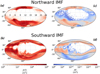 |
Fig. 1 Electron precipitation maps at the surface of Mercury using Mollweide projection. Panels a and b show the number fluxes in units of electrons cm−2 s. Panels c and d show the energy fluxes in units of eV cm−2 s. The vertical axis corresponds to geographical latitude and the horizontal axis corresponds to local time (as indicated in panel a, 12 is the subsolar longitude). Dashed black lines show the boundary between open and closed magnetic field lines (i.e., the cusps). |
3 Results
3.1 Properties of electron precipitation on the planet’s surface
In both simulations, the global system reaches a quasi-steady state after a time T ≈ 10 s. This timescale T is comparable to the Dungey cycle period in our scaled-down Mercury. In our model, scaling down the magnetosphere size by a factor 10 corresponds to scaling down the Dungey cycle period from ≈2 min to ≈10 s. Starting from this time T, we integrate the plasma precipitation on the planet’s surface for a time interval Δt = 50 ms, corresponding to about two electron gyro-periods (τce = 2π/ωce = 30 ms in our simulations with the chosen electron mass rescaling). From the precipitated plasma, we compute the electron precipitation maps shown in Fig. 1. Moreover, solarwind ion precipitation maps in the same format as Fig. 1 can be found in Appendix B. The precipitation maps are obtained using a total of ~106 macro-particles, enabling a good representation of the electron energy distribution function at the surface. Data concerning the macro-particles collected onto the surface are publicly available at this link1.
The electron precipitation maps in Fig. 1 show significant spatial inhomogeneities for both explored IMF configurations. In the case of northward IMF (RunN), the solar-wind electrons are (i) energized up to energies of a few keV and (ii) concentrated onto the northern and southern cusps. In RunN, the northern cusp extends down to a latitude of ~+60° while the southern cusp extends to a latitude of ~−30°. Such north-south asymmetry is due to the northward shift of the planetary magnetic dipole. Energy fluxes in the cusps reach values of ~1012 eV cm−2 s, two orders of magnitude higher than in the pristine solar wind (see Table 1). In the case of southward IMF (RunS), high-energy electrons (up to few keV) precipitate at low latitudes close to the magnetic equator (from −50° to +60°) and mainly at the nightside. This energy flux is higher on the dawn side (LT 0–6 h) than on the dusk side (LT 18–24 h), in agreement with indirect electron observations by MESSENGER (Baker et al. 2016; Dewey et al. 2018; Lindsay et al. 2016). Possible drivers of such an electron enhancement at dawn are (i) the dawn-ward drift of electrons injected from the neutral line in the tail toward the planet (Christon 1987; Dong et al. 2019; Lavorenti et al. 2022) and (ii) the enhanced magnetic reconnection at dawn in the plasma sheet (Sun et al. 2022a, Chap. 4 therein). In RunS, low-energy electrons (around tens of eV) precipitate around the northern and southern poles. These electrons precipitate directly from the solar wind onto the surface without crossing the reconnection region.
We find that 1.5 times more electrons precipitate on the surface in RunS than in RunN. The rate of precipitating electrons is 1.7 × 1025 s−1 (2.6 × 1025 s−1) in RunN (RunS), corresponding to an effective area of 2% (3%) of the total 4π planet surface area. The rates, fluxes, and energies reported here are in agreement with the findings of Schriver et al. (2011a). For unmagnetized bodies (such as Mars, Venus, comets, or the Moon), the effective area exposed to solar wind is 50% of the body’s surface area given the absence of any magnetic field shielding. In those cases, precipitation is much higher as compared to Mercury, but the solar wind does not suffer acceleration in the magnetosphere (Kallio et al. 2008). A weak magnetic field, like that of Mercury, therefore (i) filters the solar-wind in precise regions of the surface and (ii) accelerates the incoming electrons by around a factor 100 in energy. Both effects (filtering and acceleration) are not possible around unmagnetized objects.
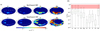 |
Fig. 2 Electron impact ionization rates in Mercury’s exosphere. Panel a: maps in the same format as Fig. 1 of EII rates of exosphere H, He, O, and Mn. Panel b: box-plot of the distribution of EII-to-photoionization frequency ratios for multiple exosphere species (RunN and RunS are merged). The red box highlights the region of significant EII rates. |
3.2 Interaction of precipitating electrons with the exosphere and surface
Before hitting the rocky surface of the planet, electrons interact with the exosphere. We address the efficiency of electron impact ionization (EII) of multiple exosphere species using the electron energy distribution from our simulations, because we want to assess the relevance of EII (usually considered a secondary, negligible effect) in comparison to photoionization (the primary ionization process). The distribution of EII rates computed from Eq. (1) over the planet’s surface is shown in Fig. 2a for hydrogen (H), helium (He), oxygen (O), and manganese (Mn) for both simulation runs. Moreover, maps of EII rates for all exosphere species considered in this work can be found in Appendix C in the same format as Fig. 2a. These four species have the highest EII-to-photoionization frequency ratio, as shown in Fig. 2b (photoionization rates vph are taken from Huebner & Mukherjee (2015) for quiet sun conditions and rescaled to Mercury’s aphelion). For H, He, O, and Mn, EII is relevant (i) in the dayside, where locally vEII ≈ vph and (ii) in the nightside, where ionization of neutrals is dominated by EII with typical rates of ~0.1 vph. Differently from photoionization, EII is (i) localized on specific regions of the surface and (ii) strongly dependent on the upstream solar-wind parameters, as shown in Fig. 2a. Variations in the IMF direction, such as moving from northward to southward IMF, induce strong variations in EII rates locally at the surface. We also show that EII of sodium (Na), magnesium (Mg), aluminum (Al), silicon (Si), potassium (K), and calcium (Ca) are negligible under nominal solar-wind conditions, as shown in Fig. 2b. This result supports the common assumption of negligible EII for the Na exosphere (Sun et al. 2022b; Jasinski et al. 2021). Nevertheless, compared to photoionization, EII should not be considered a secondary process for the H, He, O, and Mn exosphere.
When hitting the surface, electrons induce the emission of photons from the surface atoms via X-ray fluorescence (XRF). This latter is driven by electrons with energies above a few hundred eV (Bunce et al. 2020, Table 5 therein). From the electron energy distribution at the surface obtained from our simulations, we compute the flux of emitted X-rays ℱXRF from Eq. (2), as shown in Fig. 3a. We include XRF emission from the most abundant species on Mercury’s surface, namely O, Na, Mg, Al, Si, S, Ca, and Fe. Figure 3b shows the relative intensity of each of the X-ray emission lines from these different elements. We find that electron-induced X-ray emissions from the surface of Mercury present strong spatial inhomogeneities dependent upon the upstream IMF conditions. Regions of strongest X-ray emission correspond to regions of high-energy electron precipitation, namely the poles (in the case of northward IMF) and the low-latitude, dawn-midnight sector (in the case of southward IMF). In these regions, the emitted X-ray flux reaches values of the order of 107 photons cm−2 s−1 (mostly coming from the O-Kα line). The MESSENGER/XRS instrument was able to measure X-rays from Si- and Ca-group ions at Mercury’s nightside (Lindsay et al. 2016), and partially at the dayside (Lindsay et al. 2022) during periods of low solar activity. Due to limited energy range and energy resolution, XRS was not able to measure the rich variety of emission lines obtained from our simulations shown in Fig. 3b. Our results corroborate the idea – built upon MESSENGER observations - that Mercury’s X-ray aurora-like emission is due to high-energy electron precipitation at the surface. Moreover, our modeled X-ray flux provides a new means to interpret and plan future in situ observations by the BepiColombo/MIXS instrument (Bunce et al. 2020). The integrated X-ray luminosity of Mercury from electron-induced XRF is ℒ ≈ 1024 photons s−1. Such luminosity is comparable to that of other Solar System bodies shining in X-rays (Bhardwaj et al. 2007), such as comets, Jupiter, and Saturn. Nonetheless, remote observations from Earth of Mercury’s X-ray aurora remain challenging due to the strong background of X-ray photons coming from the Sun.
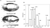 |
Fig. 3 X-ray emissions from the surface of Mercury induced from high-energy electron precipitation. Panel a: maps (same format as Fig. 1) showing the total X-ray photon flux emitted from the surface in our two runs, as computed in Eq. (2). Panel b: INTENSITY of the different X-ray emission lines considered in this study. The intensity of these lines corresponds to the surface integral of the X-ray photon flux FXRFs in Eq. (2). To better visualize the lines, a Gaussian profile with a width of 5 eV is used. |
4 Conclusions
To conclude, using a novel, fully kinetic 3D approach, we investigated the properties of solar-wind electron precipitation on the surface of Mercury-like bodies. The magnetosphere of those bodies acts (i) as a shield, allowing only a few percent of the solar wind to precipitate onto the surface and (ii) as an accelerator, increasing electron energies by a factor ~100. Using the self-consistently modeled electron precipitation fluxes as the input to exosphere and surface impact processes, we find two main results.
First, electron impact ionization of exospheric H, He, O, and Mn at Mercury is shown to be an efficient process. On the dayside, electron impact ionization is locally as efficient as photoionization. On the nightside, it is the dominant source of ionization of neutrals because photoionization is inhibited. The ionization rates provided here are crucial to complement fluid and hybrid models of Mercury’s environment, which cannot model electron acceleration processes.
Second, electrons accelerated in the magnetosphere induce X-ray emission from the surface with fluxes of the order of 107 photons cm−2 s−1, mostly from surface oxygen. This result corroborates and provides the physical origin of the X-ray aurora-like emissions observed by the MESSENGER/XRS instrument; it also paves the way for the future planning of BepiColombo/MIXS observations.
Acknowledgements
This work was granted access to HPC resources at TGCC under the allocation A0100412428 and A0120412428 made by GENCI via the DARI procedure. We acknowledge the CINECA award under the ISCRA initiative, for the availability of high performance computing resources and support for the project IsC93. We acknowledge the support of CNES for the BepiColombo mission. Part of this work was inspired by discussions within International Team 525: “Modelling Mercury’s Dynamic Magnetosphere in Anticipation of BepiColombo” at the International Space Science Institute, Bern, Switzerland. We acknowledge support by ESA within the PhD project “Global modelling of Mercury’s outer environment to prepare BepiColombo”. J.D. gratefully acknowledges support from NASA’s Solar System Exploration Research Virtual Institute (SSERVI): Institute for Modeling Plasmas, Atmosphere, and Cosmic Dust (IMPACT), the NASA High-End Computing (HEC) Program through the NASA Advanced Supercomputing (NAS) Division at Ames Research Center, and NASA’s Rosetta Data Analysis Program, Grant No. 80NSSC19K1305. The part of this work carried by S.A. is supported by JSPS KAKENHI number: 22J01606.
Appendix A Fully kinetic simulations: Impact of rescaling
In our fully-kinetic simulations, we rescale the ion-to-electron mass ratio mi/me, the plasma-to-cyclotron frequency ratio ωpi/ωci, and the normalized planet radius R in order to be able to run the simulations on state-of-the-art HPC facilities while maintaining a good scale separation between electron, ion, and planetary scales. We are confident that the use of such rescaled parameters does not qualitatively alter the physical processes at play in our simulations.
On state-of-the-art HPC facilities, computational constraints impose the use of rescaled parameters to run fully kinetic simulations of large systems, such as Mercury’s magnetosphere. If such rescalings are done “carefully”, the modeled environment is still representative of the real one to a good degree of approximation, as demonstrated by the large number of publications for similar systems using reduced parameters. The exact meaning of “carefully” strongly depends on the plasma process under consideration. In the following, we address the impact of each of the rescaled parameters on the simulation results. In Sect. A.1, we show how the rescalings of mi/me and ωpi/ωci affect the microphysics in fully kinetic simulations while leaving the large-scale structure unchanged. In Sect. A.2, we discuss the role of a reduced planet radius on the results of global plasma simulations of planetary systems.
A.1 Effects of mi/me and ωpi/ωci on the microphysics
Fully kinetic simulations of space plasmas are commonly performed using (i) a reduced mass ratio mi/me of the order of 25 – 400 (Karimabadi et al. 2013; Deca et al. 2017, 2018; Pucci et al. 2018; Parashar et al. 2018; Olshevsky et al. 2018; Deca et al. 2019; Lapenta et al. 2020; Vega et al. 2020; Pezzi et al. 2021; Bacchini et al. 2022; Arró et al. 2022; Lavorenti et al. 2022) instead of the real hydrogen proton-to-electrom mass ratio of 1836, and (ii) a reduced ωpi/ωci ratio of the order of 10–500 (Karimabadi et al. 2013; Saito & Nariyuki 2014; Parashar et al. 2015b,a; Grošelj et al. 2018; Parashar & Gary 2019; Roytershteyn et al. 2019) instead of more realistic values of the order of 103–104 found typically in the solar wind. These two choices allow one to reduce the computational time needed to simulate a system of a given size. Indeed, the computational time of a fully kinetic simulation with fixed system size, grid resolution dx ~ de, time step  , and time
  scales as:
 (A.1)
(A.1)
where D is the number of spatial dimensions of the system. Therefore, the rescalings typically operated on mi/me and ωpi/ωci reduce the computational time by several orders of magnitude.
Magnetic reconnection is a fundamental plasma process that regulates the energization and circulation of plasma in the magnetosphere of the Earth (Dungey 1961) and, to a similar extent, in that of Mercury (Slavin et al. 2010; Dibraccio et al. 2013). The impact of rescaled parameters on magnetic reconnection has been extensively investigated in past numerical works (Shay & Drake 1998; Hesse et al. 1999) that only had access to limited computational resources. There, the authors showed that rescaled parameters only affect the microphysics of the system while leaving the large-scale quantities, such as the reconnection rate, unchanged. Indeed, an increased electron mass impacts the electron distribution function in the electron diffusion region very locally around the X-point, but leaves the plasma parameters of the outflow unchanged. In particular, electron acceleration by magnetic reconnection is weakly affected by the mass ratio mi/me far from the X-point (Hesse et al. 1999; Haggerty et al. 2015). Magnetic reconnection with guide field is more strongly affected by a reduced ion-to-electron mass ratio (Le et al. 2013), but this is not the case in our simulations, where there is no guide field since the IMF is purely northward or southward. Based on the results of these past works, we expect a negligible impact of the rescaled parameters mi/me and ωpi/ωci on magnetic reconnection in our simulations of Mercury’s magnetosphere.
In the interaction between the solar wind and Mercury’s magnetosphere, multiple plasma waves are also excited. In principle, these waves can be affected by the rescalings of mi/me and ωpi/ωci both in their linear phase and in their corresponding nonlinear dynamics. A comprehensive study of the impact of these rescalings on the nonlinear dynamics of plasma waves is extremely challenging. On the other hand, Verscharen et al. (2020) studied the linear dependence of multiple plasma waves on the parameters mi/me and ωpi/ωci·. There, the authors showed that plasma models with mi/me ≳ 100 and ωpi/ωci ≳ 10 (as it is in our case) successfully represents the physics at scales above ≳ 0.2 di (which corresponds to 2dx in our simulations). Analogous results were obtained by Bret & Dieckmann (2010) studying the impact of mi/me on beam-plasma instabilities. There, the authors concluded that simulations with mi/me ≳ 100 preserve the hierarchy of the linearly unstable modes and are therefore a good representation of the system.
A.2 Effect of a reduced planet radius
Global fully kinetic simulations of a large system, such as a planetary magnetosphere, are extremely challenging. The large scale separation between the magnetosphere size (at Mercury the magnetopause standoff distance is dMP ≈ 1.5 R ≈ 4 · 103 km) and the ion scale (in the solar wind at Mercury di ≈ 50 km) makes simulations of a real-sized planetary magnetosphere computationally very expensive. The computational time of a simulation with fixed grid resolution, fixed time step, system size L ~ dMP, and time T ~ L/Vsw scales as:
 (A.2)
(A.2)
where D is the number of spatial dimensions of the system. Therefore, a reduction of the normalized planet radius R → εR reduces the computational time by several orders of magnitude. This rescaling preserves the ratio dMP/R because the magnetic moment of the planet is also reduced by a factor ε3. In our simulations, we use ε = 0.1 to obtain a reduction in computational time of four orders of magnitude while keeping a good separation between ion kinetic scales (in the solar wind the ion gyroradius is ρi ≈ 23 km) and planetary scales (the reduced planet radius is R ≈ 230 km).
This rescaling technique was first introduced by Trávníček et al. (2007) for the study of Mercury using global 3D hybrid simulations. There, the authors showed that global simulations using a reduced planet radius (in their case ε ≈ 0.2) enable a good representation of the real system and provide useful insight into the global kinetic ion dynamics in the magnetosphere. Further works by those authors using a reduced planet radius have led to important results on the magnetosphere of Mercury in support of MESSENGER observations; see for instance Trávníček et al. (2009, 2010); Herčík et al. (2013, 2016); Schriver et al. (2011b).
On the one hand, the increased computational power of present HPC facilities (compared to those of 10–15 years ago) has enabled researchers to run global 3D hybrid simulations of Mercury using a real-sized planet (Fatemi et al. 2018; Exner et al. 2018; Aizawa et al. 2020). On the other hand, present state-of-the-art HPC facilities still do not allow global fully-kinetic simulations to be run using a real-sized planet (a computational gap that might be filled in 10–15 years as happened with hybrid simulations). Nonetheless, at present, fully kinetic simulations of the magnetosphere of Mercury are key to planning and interpreting in situ observations by BepiColombo, which is the first mission to address electron scale dynamics at Mercury.
Some authors tried to assess the impact of this planet rescaling on global magnetospheres. Omidi et al. (2004) identified different magnetosphere structures for different values of the normalized magnetopause standoff distance Dp = dMP /di using 2D global hybrid simulations. At Mercury, this parameter is of the order of Dp ~ 1.5 R/di ~ 100. There, the authors found that values Dp ~ 20 or greater correspond to an Earth-like magnetosphere structure. Tóth et al. (2017) characterized the minimal rescaling factor ε to run global 3D simulations representative of Earth’s magnetosphere using MHD simulations with embedded PIC regions. There, the authors found that, for Earth, a reduction factor of ε ≳ 1/32 yields comparable magnetosphere structures and dynamics.
We expect a negligible impact of the planet rescaling on electron adiabatic energization processes. Electrons in the magnetosphere undergo adiabatic betatron and Fermi acceleration while streaming towards the planet and along magnetic field lines, respectively. These processes are well modeled for electrons in our simulations given the large separation between planetary and electron scales (see also the discussion in Lavorenti et al. (2022)). On the contrary, for ions, adiabatic processes can only be poorly modeled in our simulations given the marginal separation between planetary and ion scales in some regions of the scaled-down magnetosphere.
Appendix B Ion precipitation maps on the surface
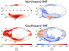 |
Fig. B.1 Ion precipitation maps (same format as Fig. 1) obtained from our fully kinetic simulations. These maps can be used for comparison with other works addressing proton precipitation at Mercury with hybrid models. |
Appendix C Complete set of EII rate surface maps
 |
Fig. C.1 Full set of EII rates maps (same format as Fig. 2a) for all neutral species considered in this work. These maps are used to build the boxplot in Fig. 2b. |
References
- Aizawa, S., Delcourt, D., Terada, N., & André, N. 2020, Planet. Space Sci., 193, 105079 [NASA ADS] [CrossRef] [Google Scholar]
- Anderson, B. J., Johnson, C. L., Korth, H., et al. 2012, J. Geophys. Res. (Planets), 117, E00L12 [Google Scholar]
- Arró, G., Califano, F., & Lapenta, G. 2022, A&A, 668, A33 [NASA ADS] [CrossRef] [EDP Sciences] [Google Scholar]
- Bacchini, F., Pucci, F., Malara, F., & Lapenta, G. 2022, Phys. Rev. Lett., 128, 025101 [NASA ADS] [CrossRef] [Google Scholar]
- Baker, D. N., Dewey, R. M., Lawrence, D. J., et al. 2016, J. Geophys. Res. (Space Phys.), 121, 2171 [NASA ADS] [CrossRef] [Google Scholar]
- Benkhoff, J., Murakami, G., Baumjohann, W., et al. 2021, Space Sci. Rev., 217, 90 [NASA ADS] [CrossRef] [Google Scholar]
- Bhardwaj, A., Elsner, R. F., Randall Gladstone, G., et al. 2007, Planet. Space Sci., 55, 1135 [Google Scholar]
- Bret, A., & Dieckmann, M. E. 2010, Phys. Plasmas, 17, 032109 [NASA ADS] [CrossRef] [Google Scholar]
- Bunce, E. J., Martindale, A., Lindsay, S., et al. 2020, Space Sci. Rev., 216, 126 [NASA ADS] [CrossRef] [Google Scholar]
- Christon, S. P. 1987, Icarus, 71, 448 [NASA ADS] [CrossRef] [Google Scholar]
- Deca, J., Divin, A., Henri, P., et al. 2017, Phys. Rev. Lett., 118, 205101 [Google Scholar]
- Deca, J., Divin, A., Lue, C., Ahmadi, T., & Horányi, M. 2018, Commun. Phys., 1, 12 [CrossRef] [Google Scholar]
- Deca, J., Henri, P., Divin, A., et al. 2019, Phys. Rev. Lett., 123, 055101 [Google Scholar]
- Dewey, R. M., Raines, J. M., Sun, W., Slavin, J. A., & Poh, G. 2018, Geophys. Res. Lett., 45, 10, 110 [NASA ADS] [Google Scholar]
- Dibraccio, G. A., Slavin, J. A., Boardsen, S. A., et al. 2013, J. Geophys. Res. (Space Phys.), 118, 997 [NASA ADS] [CrossRef] [Google Scholar]
- Dong, C., Wang, L., Hakim, A., et al. 2019, Geophys. Res. Lett., 46, 11, 584 [NASA ADS] [Google Scholar]
- Dungey, J. W. 1961, Phys. Rev. Lett., 6, 47 [NASA ADS] [CrossRef] [Google Scholar]
- Exner, W., Heyner, D., Liuzzo, L., et al. 2018, Planet. Space Sci., 153, 89 [NASA ADS] [CrossRef] [Google Scholar]
- Fatemi, S., Poirier, N., Holmström, M., et al. 2018, A&A, 614, A132 [NASA ADS] [CrossRef] [EDP Sciences] [Google Scholar]
- Fatemi, S., Poppe, A. R., & Barabash, S. 2020, J. Geophys. Res. (Space Phys.), 125, e27706 [NASA ADS] [Google Scholar]
- Golyatina, R. I., & Maiorov, S. A. 2021, Atoms, 9, 90 [CrossRef] [Google Scholar]
- Groselj, D., Mallet, A., Loureiro, N. F., & Jenko, F. 2018, Phys. Rev. Lett., 120, 105101 [CrossRef] [Google Scholar]
- Haggerty, C. C., Shay, M. A., Drake, J. F., Phan, T. D., & McHugh, C. T. 2015, Geophys. Res. Lett., 42, 9657 [Google Scholar]
- Herčík, D., Trávníček, P. M., Johnson, J. R., Kim, E.-H., & Hellinger, P. 2013, J. Geophys. Res. (Space Phys.), 118, 405 [CrossRef] [Google Scholar]
- Herčík, D., Trávníček, P. M., Åtverák, Å. T., & Hellinger, P. 2016, J. Geophys. Res. (Space Phys.), 121, 413 [CrossRef] [Google Scholar]
- Hesse, M., Schindler, K., Birn, J., & Kuznetsova, M. 1999, Phys. Plasmas, 6, 1781 [NASA ADS] [CrossRef] [Google Scholar]
- Ho, G. C., Krimigis, S. M., Gold, R. E., et al. 2011, Science, 333, 1865 [NASA ADS] [CrossRef] [Google Scholar]
- Ho, G. C., Krimigis, S. M., Gold, R. E., et al. 2012, J. Geophys. Res.: Space Phys., 117 [Google Scholar]
- Ho, G. C., Starr, R. D., Krimigis, S. M., et al. 2016, Geophys. Res. Lett., 43, 550 [NASA ADS] [CrossRef] [Google Scholar]
- Huebner, W., & Mukherjee, J. 2015, Planet. Space Sci., 106, 11 [Google Scholar]
- Huovelin, J., Vainio, R., Kilpua, E., et al. 2020, Space Sci. Rev., 216, 94 [NASA ADS] [CrossRef] [Google Scholar]
- James, M. K., Imber, S. M., Bunce, E. J., et al. 2017, J. Geophys. Res.: Space Phys., 122, 7907 [NASA ADS] [CrossRef] [Google Scholar]
- Jasinski, J. M., Cassidy, T. A., Raines, J. M., et al. 2021, Geophys. Res. Lett., 48, e92980 [NASA ADS] [CrossRef] [Google Scholar]
- Kallio, E., & Janhunen, P. 2003, Ann. Geophys., 21, 2133 [NASA ADS] [CrossRef] [Google Scholar]
- Kallio, E., Wurz, P., Killen, R., et al. 2008, Planet. Space Sci., 56, 1506 [NASA ADS] [CrossRef] [Google Scholar]
- Karimabadi, H., Roytershteyn, V., Wan, M., et al. 2013, Phys. Plasmas, 20, 012303 [Google Scholar]
- Kim, Y.-K., Irikura, K. K., Rudd, M. E., et al. 2005, Electron-Impact Ionization Cross Section for Ionization and Excitation Database, Version 3.0 (National Institute of Standards and Technology, Gaithersburg, Maryland) [Google Scholar]
- Lapenta, G., Pucci, F., Goldman, M. V., & Newman, D. L. 2020, ApJ, 888, 104 [Google Scholar]
- Lavorenti, F., Henri, P., Califano, F., Aizawa, S., & André, N. 2021, A&A, 652, A20 [NASA ADS] [CrossRef] [EDP Sciences] [Google Scholar]
- Lavorenti, F., Henri, P., Califano, F., et al. 2022, A&A, 664, A133 [NASA ADS] [CrossRef] [EDP Sciences] [Google Scholar]
- Lawrence, D. J., Anderson, B. J., Baker, D. N., et al. 2015, J. Geophys. Res. (Space Phys.), 120, 2851 [NASA ADS] [CrossRef] [Google Scholar]
- Le, A., Egedal, J., Ohia, O., et al. 2013, Phys. Rev. Lett., 110, 135004 [NASA ADS] [CrossRef] [Google Scholar]
- Lindsay, S. T., James, M. K., Bunce, E. J., et al. 2016, Planet. Space Sci., 125, 72 [NASA ADS] [CrossRef] [Google Scholar]
- Lindsay, S. T., Bunce, E. J., Imber, S. M., et al. 2022, J. Geophys. Res. (Space Phys.), 127, e29675 [NASA ADS] [Google Scholar]
- Llovet, X., Salvat, F., Bote, D., et al. 2014, NIST Database of Cross Sections for Inner-Shell Ionization by Electron or Positron Impact, Version 1.0 (Gaithersburg, Maryland: National Institute of Standards and Technology) [Google Scholar]
- Markidis, S., Lapenta, G., & Rizwan-Uddin 2010, Math. Comput. Simul., 80, 1509 [CrossRef] [Google Scholar]
- McCoy, T. J., Peplowski, P. N., McCubbin, F. M., & Weider, S. Z. 2018, The Geochemical and Mineralogical Diversity of Mercury, eds. S. C. Solomon, L. R. Nittler, & B. J. Anderson, Cambridge Planetary Science (Cambridge University Press), 176 [Google Scholar]
- Milillo, A., Fujimoto, M., Kallio, E., et al. 2010, Planet. Space Sci., 58, 40 [NASA ADS] [CrossRef] [Google Scholar]
- Milillo, A., Fujimoto, M., Murakami, G., et al. 2020, Space Sci. Rev., 216, 93 [NASA ADS] [CrossRef] [Google Scholar]
- Ogilvie, K. W., Scudder, J. D., Vasyliunas, V. M., Hartle, R. E., & Siscoe, G. L. 1977, J. Geophys. Res., 82, 1807 [NASA ADS] [CrossRef] [Google Scholar]
- Olshevsky, V., Servidio, S., Pucci, F., Primavera, L., & Lapenta, G. 2018, ApJ, 860, 11 [Google Scholar]
- Omidi, N., Blanco-Cano, X., Russell, C. T., & Karimabadi, H. 2004, Adv. Space Res., 33, 1996 [NASA ADS] [CrossRef] [Google Scholar]
- Parashar, T. N., & Gary, S. P. 2019, ApJ, 882, 29 [Google Scholar]
- Parashar, T. N., Matthaeus, W. H., Shay, M. A., & Wan, M. 2015a, ApJ, 811, 112 [NASA ADS] [CrossRef] [Google Scholar]
- Parashar, T. N., Salem, C., Wicks, R. T., et al. 2015b, J. Plasma Phys., 81, 905810513 [NASA ADS] [CrossRef] [Google Scholar]
- Parashar, T. N., Matthaeus, W. H., & Shay, M. A. 2018, ApJ, 864, L21 [NASA ADS] [CrossRef] [Google Scholar]
- Pezzi, O., Liang, H., Juno, J. L., et al. 2021, MNRAS, 505, 4857 [NASA ADS] [CrossRef] [Google Scholar]
- Pucci, F., Matthaeus, W. H., Chasapis, A., et al. 2018, ApJ, 867, 10 [Google Scholar]
- Richer, E., Modolo, R., Chanteur, G. M., Hess, S., & Leblanc, F. 2012, J. Geophys. Res. (Space Phys.), 117, A10228 [Google Scholar]
- Roytershteyn, V., Boldyrev, S., Delzanno, G. L., et al. 2019, ApJ, 870, 103 [Google Scholar]
- Saito, S., & Nariyuki, Y. 2014, Phys. Plasmas, 21, 042303 [NASA ADS] [CrossRef] [Google Scholar]
- Saito, Y., Delcourt, D., Hirahara, M., et al. 2021, Space Sci. Rev., 217, 70 [NASA ADS] [CrossRef] [Google Scholar]
- Schriver, D., Trávníček, P., Ashour-Abdalla, M., et al. 2011a, Planet. Space Sci., 59, 2026 [NASA ADS] [CrossRef] [Google Scholar]
- Schriver, D., Trávníček, P. M., Anderson, B. J., et al. 2011b, Geophys. Res. Lett., 38 [Google Scholar]
- Shay, M. A., & Drake, J. F. 1998, Geophys. Res. Lett., 25, 3759 [NASA ADS] [CrossRef] [Google Scholar]
- Slavin, J. A., Lepping, R. P., Wu, C.-C., et al. 2010, Geophys. Res. Lett., 37, L02105 [Google Scholar]
- Solomon, S. C., McNutt, R. L., Gold, R. E., & Domingue, D. L. 2007, Space Sci. Rev., 131, 3 [NASA ADS] [CrossRef] [Google Scholar]
- Sun, W., Dewey, R. M., Aizawa, S., et al. 2022a, Sci. China Earth Sci., 65, 25 [NASA ADS] [CrossRef] [Google Scholar]
- Sun, W., Slavin, J. A., Milillo, A., et al. 2022b, J. Geophys. Res. (Space Phys.), 127, e30280 [NASA ADS] [Google Scholar]
- Tóth, G., Chen, Y., Gombosi, T. I., et al. 2017, J. Geophys. Res.: Space Phys., 122, 10, 336 [Google Scholar]
- Trávníček, P., Hellinger, P., & Schriver, D. 2007, Geophys. Res. Lett., 34, L05104 [Google Scholar]
- Trávníček, P. M., Hellinger, P., Schriver, D., et al. 2009, Geophys. Res. Lett., 36, L07104 [Google Scholar]
- Trávníček, P. M., Schriver, D., Hellinger, P., et al. 2010, Icarus, 209, 11 [CrossRef] [Google Scholar]
- Vega, C., Roytershteyn, V., Delzanno, G. L., & Boldyrev, S. 2020, ApJ, 893, L10 [Google Scholar]
- Verscharen, D., Parashar, T. N., Gary, S. P., & Klein, K. G. 2020, MNRAS, 494, 2905 [NASA ADS] [CrossRef] [Google Scholar]
- Walsh, B. M., Ryou, A. S., Sibeck, D. G., & Alexeev, I. I. 2013, J. Geophys. Res. (Space Phys.), 118, 1992 [NASA ADS] [CrossRef] [Google Scholar]
- Wurz, P., & Blomberg, L. 2001, Planet. Space Sci., 49, 1643 [NASA ADS] [CrossRef] [Google Scholar]
- Zatsarinny, O., Parker, H., & Bartschat, K. 2019, Phys. Rev. A, 99, 012706 [NASA ADS] [CrossRef] [Google Scholar]
All Tables
Common numerical parameters of RunN and RunS with purely northward and southward IMF, respectively.
All Figures
|
Fig. 1 Electron precipitation maps at the surface of Mercury using Mollweide projection. Panels a and b show the number fluxes in units of electrons cm−2 s. Panels c and d show the energy fluxes in units of eV cm−2 s. The vertical axis corresponds to geographical latitude and the horizontal axis corresponds to local time (as indicated in panel a, 12 is the subsolar longitude). Dashed black lines show the boundary between open and closed magnetic field lines (i.e., the cusps). |
| In the text | |
|
Fig. 2 Electron impact ionization rates in Mercury’s exosphere. Panel a: maps in the same format as Fig. 1 of EII rates of exosphere H, He, O, and Mn. Panel b: box-plot of the distribution of EII-to-photoionization frequency ratios for multiple exosphere species (RunN and RunS are merged). The red box highlights the region of significant EII rates. |
| In the text | |
|
Fig. 3 X-ray emissions from the surface of Mercury induced from high-energy electron precipitation. Panel a: maps (same format as Fig. 1) showing the total X-ray photon flux emitted from the surface in our two runs, as computed in Eq. (2). Panel b: INTENSITY of the different X-ray emission lines considered in this study. The intensity of these lines corresponds to the surface integral of the X-ray photon flux FXRFs in Eq. (2). To better visualize the lines, a Gaussian profile with a width of 5 eV is used. |
| In the text | |
|
Fig. B.1 Ion precipitation maps (same format as Fig. 1) obtained from our fully kinetic simulations. These maps can be used for comparison with other works addressing proton precipitation at Mercury with hybrid models. |
| In the text | |
|
Fig. C.1 Full set of EII rates maps (same format as Fig. 2a) for all neutral species considered in this work. These maps are used to build the boxplot in Fig. 2b. |
| In the text | |
Current usage metrics show cumulative count of Article Views (full-text article views including HTML views, PDF and ePub downloads, according to the available data) and Abstracts Views on Vision4Press platform.
Data correspond to usage on the plateform after 2015. The current usage metrics is available 48-96 hours after online publication and is updated daily on week days.
Initial download of the metrics may take a while.