| Issue |
A&A
Volume 674, June 2023
|
|
|---|---|---|
| Article Number | A50 | |
| Number of page(s) | 13 | |
| Section | Planets and planetary systems | |
| DOI | https://doi.org/10.1051/0004-6361/202245316 | |
| Published online | 31 May 2023 | |
Clustering the properties of near-Earth objects: physico-dynamical links among NEOs★
1
INAF Osservatorio Astronomico di Roma,
Via Frascati 33,
00078
Monte Porzio Catone, Roma, Italy
e-mail: This email address is being protected from spambots. You need JavaScript enabled to view it.
2
Department of Earth, Atmospheric and Planetary Sciences, Purdue University,
West Lafayette, IN
47907, USA
3
Department of Physics,
PO Box 64,
00014
University of Helsinki,
Finland
4
Asteroid Engineering Laboratory, Luleå University of Technology,
Box 848,
981 28
Kiruna, Sweden
5
LESIA-Observatoire de Paris, Université PSL, CNRS, Sorbonne Université, Université de Paris,
5 place Jules Janssen,
92195
Meudon, France
6
Agenzia Spaziale Italiana,
Via del Politecnico 1,
00133
Rome, Italy
Received:
28
October
2022
Accepted:
30
March
2023
Abstract
Context. At present, near-Earth objects (NEOs) are being discovered at an ever-increasing rate. However, their physical characterisation is still significantly lagging behind. In particular, the taxonomic classification of newly discovered NEOs is of great importance with regard to improving our understanding of the population of NEOs.
Aims. In this context, our goal is to probe potential links between orbital properties of NEOs and their composition. We investigate whether we can make a reasonable guess about the taxonomic class of an NEO upon its discovery with a decent orbital accuracy.
Methods. We used a G-mode multivariate statistical clustering method to find homogeneous clusters in a dataset composed of orbital elements of NEOs. We adopted two approaches, using two sets of variables as inputs to the G-mode method. In each approach, we analysed the available taxonomic distribution of resulting clusters to find potential correlations with several unique parameters that distinctively characterise NEOs. We then applied a dynamical model on the same clusters to trace their escape regions.
Results. Approach 1 (A1) led us to obtain NEO clusters that can be linked to a primitive composition. This result was further strengthened by the dynamical model, which mapped outer-belt sources as escape regions for these clusters. We remark on the finding of a cluster akin to S-type NEOs in highly eccentric orbits during the same approach (A1). Two clusters, one with small NEOs in terrestriallike orbits and one with relatively high inclinations, were found to be common to both approaches. Approach 2 (A2) revealed three clusters that are only separable by their arguments of perihelion. Taken altogether, they make up the majority of known Atira asteroids.
Conclusions. For an NEO whose orbit is relatively well determined, we propose a model to determine whether the taxonomy of an NEO is siliceous or primitive if the orbital elements of the NEO fall within the presented combinations of inclination, eccentricity, and semi-major axis ranges.
Key words: minor planets / asteroids: general / techniques: spectroscopic / methods: statistical
The NEO dataset is only available at the CDS via anonymous ftp to cdsarc.cds.unistra.fr (130.79.128.5) or via https://cdsarc.cds.unistra.fr/viz-bin/cat/J/A+A/674/A50
© The Authors 2023
 Open Access article, published by EDP Sciences, under the terms of the Creative Commons Attribution License (https://creativecommons.org/licenses/by/4.0), which permits unrestricted use, distribution, and reproduction in any medium, provided the original work is properly cited.
This article is published in open access under the Subscribe to Open model. This email address is being protected from spambots. You need JavaScript enabled to view it. to support open access publication.
1 Introduction
Asteroids are characterised by a dynamic spectrum of varying compositions and spectral taxonomies across heliocentric distances. Due to the Yarkovsky force and orbital resonances with giant planets, some asteroids or collisional fragments of asteroids end up leaving the main asteroid belt and arrive in the vicinity of Earth, in which case they are referred to as near-Earth objects, usually referred to as NEOs (Bottke et al. 2002; Morbidelli & Vokrouhlický 2003). The study of NEOs is crucial to improving our understanding of the origin, formation, and evolution of the Solar System, and is closely linked to understanding the origins of life on Earth. Most importantly, they are time capsules that contain primitive material that is less altered, thus preserving compositional signatures of the early solar nebula. In particular, the compositional, morphological, and orbital characterisation of NEOs sheds light on the delivery of water and organics (Ehrenfreund & Sephton 2006; Altwegg et al. 2015; Marty et al. 2016) to the prebiotic Earth, while some NEOs could be potential hazards for life on Earth (Perna et al. 2013), as has been witnessed in the past (Brown et al. 2013; Popova et al. 2013). Furthermore, NEOs are of interest for the future of humankind, as they could be useful as vital resources in the course of interplanetary travel.
In this context, we seek to identify potential links between two independent properties that describe NEOs, namely, their composition and orbital elements, to grasp their physico-dynamical nature. Such an analysis becomes important due to several reasons. The known population of NEOs is growing at an exponential rate, as increasing numbers of telescopic surveys and new telescopes contribute to the effort of discovering NEOs (Jedicke et al. 2015). After an NEO gets discovered and its orbit is initially determined, the uncertainty of the orbit can be subsequently reduced following additional targeted or fortuitous observations. However, its composition (Perna et al. 2018; Binzel et al. 2019) remains unknown until dedicated spectroscopic or spectrophotometric observations are made, although the measurement of albedo could, in some cases, be used as an input to indirectly and naively infer the taxonomic class of an ΝΕΟ (Bus & Binzel 2002; DeMeo et al. 2009, 2015). The absence of a taxonomy at the discovery of an ΝΕΟ is therefore an inherited disadvantage when studying physical properties of NEOs. Therefore, we have undertaken this study to investigate whether (or to what extent) we could assign a taxonomy for an ΝΕΟ, upon its discovery, just by looking at the distribution of its orbital elements. As such, in order to probe links between the composition and orbital elements of NEOs, we applied a multivariate statistical clustering method on the currently available population of NEOs to identify homogeneous clusters of NEOs. Then we explored the distribution of available taxonomies of resulting ΝΕΟ clusters to distinguish any potential correlations. Finally, we synthesised the results by presenting a simple model of making a reasonable guess whether the taxonomy of an ΝΕΟ is primitive (or not) if its orbital elements fall in the restricted applicable range of orbital elements of the model.
2 Data and methods
2.1 NEO dataset
Our dataset of NEOs comes from the IAU Minor Planet Center (MPC)1. We queried NEOs belonging to the dynamical groups Atiras, Atens, Apollos, and Amors from the MPC and filtered them based on their uncertainty parameter (U), introduced by the MPC. The latter is an integer from 0 (least uncertainty) to 9 (highest uncertainty) and is a logarithmic measure of the longitudinal uncertainty of the mean anomaly of an orbit after a time span of 10 yr. We chose to only include NEOs with U ≤ 5 in order to select NEOs with a relatively satisfactory orbital determination for this work. We stress that this is an arbitrary choice to select objects with fairly accurate orbits and, at the same time, to maximise the number of objects with known taxonomy. This led to a sample of 14 132 NEOs and their distribution in terms of aforementioned dynamical groups can be seen on Fig. 1.
We looked for taxonomic data from published literature based on spectroscopic surveys (Perna et al. 2018; Binzel et al. 2019; Devogèle et al. 2019; Ieva et al. 2020; Simion et al. 2021; Hromakina et al. 2021) as well as spectrophotometric surveys (Lin et al. 2018). The rest of the taxonomic data are sourced from various small-body databases, which include EARN dataset2, Near-Earth Objects Coordination Centre managed by the ESA3 and the Small-Body Database of NASA. These sources yielded taxonomies for 1566 NEOs, a number that represents just over 11% of our entire sample. In Fig. 2, we show the distribution of NEOs as a function of their taxonomic compositional classification. Because of the similarity of some spectral taxonomies and with the aim of making the statistics more meaningful, we associated the F-type to Β-type taxonomy and M, E, and P-types to X-type taxonomy.
Albedo data were retrieved for NEOs whenever they were available. They were sourced mainly from the neowise dataset (Mainzer et al. 2019) and findings from the literature.
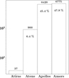 |
Fig. 1 Distribution of NEOs belonging to dynamical groups Atiras. Atens, Apollos, and Amors, included in this work. |
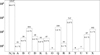 |
Fig. 2 Taxonomic distribution of NEOs included in this work. The x-axis refers to different taxonomic types and N/A corresponds to NEOs for which taxonomic data are not currently available. |
2.2 G-mode method
We then applied the G-mode multivariate statistical clustering analysis (Barucci et al. 1987, 2005; Gavrishin et al. 1992) to NEOs in our sample to identify unimodal clustering of objects with a given statistical precision. The G-mode classification method seeks to identify homogeneous clusters of objects within a sample of Ν objects (NEOs in this case), described by M variables (NEOs’ orbital elements and other ancillary parameters of choice) without a priori clustering criteria and accounts for the uncertainties of variables of each object. The method involves transformation of the input multivariate sample into a univariate sample through iterative steps. The assignment of an object to a given cluster is defined on statistical inference rules. The confidence level defines the probability of accepting the hypothesis that an object belongs to a given cluster and this is the only a priori criterion set by the user in the G-mode method. The objects assigned to each cluster follow a Gaussian distribution normalised to mean 0 and standard deviation 1. Depending on the confidence level, which corresponds to a given critical value q1, expressed in terms of σ, objects are either assigned to a cluster or discarded. For example, the critical value of q1 = 3 corresponds to classifying the entire sample with a probability of 99.7% (3σ level of the standard normal distribution) making the right decision when assigning an object to a cluster. The higher the q1, the less populous the output clusters will be and vice versa. Hence, a G-mode run will result in one or more clusters (depending on the choice of q1 and the statistical nature of the dataset) as well as a group of discarded objects generally referrable as outliers.
We refer to the aforementioned literature for a detailed mathematical description of the method and to Tosi et al. (2005); Perna et al. (2017); Barucci et al. (2019), and Bott et al. (2022) for the implementation of G-mode method in different types of datasets. We have used the python implementation of the G-mode code by Hasselmann et al. (2013) in this work.
We used two approaches in terms of input variables to the G-mode method: (1) inclination (i), eccentricity (e), and semi-major axis (a) of the orbit of a given NEO and their respective uncertainties; (2) same as (1) with the inclusion of argument of perihelion (ω), Tisserand parameter with respect to Jupiter (ΤJ), and the absolute magnitude (H) of a given NEO and their respective uncertainties. The variables i, e, and a used in the first approach effectively fix the orbit of an object in space with respect to the Sun and are primarily of a dynamic interest. The three ancillary variables ω, ΤJ, and H are included in addition in the second approach due to physical reasons. Here, H can be directly translated to the physical dimension of an NEO for an assumed albedo, while ΤJ can link NEOs on cometary-like orbits and ω can be used to identify Jupiter-family comets (JFCs) due to clusterings at ω = 0° and ω = 180° (Sosa et al. 2012). In addition, ω can be exploited to find young collisional families, as they tend to conserve ω (Carruba et al. 2018).
3 Results
First we present the results with the approach 1 (A1) with three input variables followed by those with the approach 2 (A2) with six input variables. For each G-mode run, statistics of resulting clusters are tabulated in the Appendix A. Each table is followed by a tabulation of the taxonomical distribution (subject to availability) corresponding to the given G-mode run. We note that different G-mode runs in each approach are mutually independent and, therefore, the order of the clusters may change from one G-mode run to another. To facilitate the tracking of a given cluster across G-mode runs of varying confidence levels, we refer the reader to respective sankey diagrams available for each approach.
3.1 Approach 1 (A1)
3.1.1 A1 at q1 = 3.0
We started off by applying the G-mode method to our dataset at a confidence level of 3σ (or q1=3). This resulted in only one homogeneous cluster of NEOs, denoted as C14 and the discarded group of outlier NEOs. In Table A.2, in addition to reporting the mean values of i, e, and a, which were the input parameters to the G-mode method, we have also included mean values of several ancillary parameters of interest, in order to better understand the homogeneity of clusters. These are the minimum orbital intersection distance to Earth (MOIDE), perihelion distance (q), aphelion distance (Q), Tisserand parameter with respect to Jupiter (TJ) and the absolute magnitude (H). The median absolute deviations are also reported in Table A.2 with the mean values. The fact that G-mode returned only one cluster at a confidence level of 3σ and that it contains more than 98% of the NEOs in our sample implies that the global dataset is homogeneous in terms of the three orbital elements used as inputs. We compared the mean parameters of this homogeneous cluster with those of the entire NEO population, discovered as of 27/10/2021. There are 26985 NEOs in this population and we report their statistics in Table A.1. This comparison led us to establish that this homogeneous cluster is representative of the entire population of NEOs. For brevity, from now on we refer to this cluster as the background population. The group of outliers, on the other hand, clearly differs from the background population in terms of its mean inclination, which is about 55° and its mean absolute magnitude, which is about three magnitudes brighter. We note that H remains the parameter that varies the most between entire population of discovered NEOs and the obtained cluster. This is because we restricted our input NEO sample to objects with an accurate-enough orbital determination: due to survey limitations, the largest objects (smaller H) have likely been discovered earlier and tend to have more accurate orbits.
3.1.2 A1 at q1 = 2.9
At a confidence level of 2.9σ, apart from the background population, it is possible to see the emergence of a second cluster from the sample, as reported in Table A.3. A careful comparison with the results obtained at the confidence level of 3σ reveals that the newly emerged cluster is directly related to the outliers group obtained at the confidence level of 3σ (refer to the sankey diagram on Fig. 3). In fact, the outliers group in this run at a confidence level of 2.9σ appears interesting due to its mean semi-major axis, eccentricity, and ΤJ, all of which correspond to cometary orbital elements. In particular, the mean ΤJ which is below 2, suggests that this outlier group may contain objects belonging to the family of Damocloids. Damocloids have orbits similar to those of long-period comets but without any observed outgassing and are thought to be dead or dormant cometary nuclei (Jewitt 2005). Indeed, by inspecting the individual members of this outlier group, we found that 1999 XS35, 343 158 Marsyas, 2014 PP69, 2020 BZ12 all have TJ <2 and that all have retrograde orbits except for 1999 XS35. These four NEOs represent 25% of the outliers in this G-mode run. Furthermore, 3552 Don Quixote, an NEO with D-type taxonomy and identified cometary activity (Mommert et al. 2014) was also found among the members of this outlier group. Recent work (Fatka et al. 2022) has shown using broadband photometry, that 2019 PR2 and 2019 QR6, 2 NEOs with similar orbits found in this outlier group, have a taxonomy similar to D-types. It is known that D-types are a rare taxonomy category among NEOs. These authors modeled cometary activity for this pair of NEOs and the results indicate a very recent formation (not earlier than 420 years ago). With these results, this outlier group ends up with 19% of NEOs with D-type taxonomy. Finally, we note three NEOs: 343158, 2014 PP69, 2020 BZ12 with retrograde orbits in this outlier group, which corresponds to 19% of the objects. These dynamical and compositional constraints therefore strongly suggest a cometary origin for the objects in this outlier group.
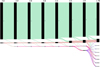 |
Fig. 3 Sankey diagram showing the transfer of objects among different clusters across G-mode runs of varying confidence levels from 3σ to 1.78σ. This diagram corresponds to the first approach where three input variables were used. The colours correspond to an Nth cluster in a given G-mode run, i.e. the second cluster of any G-mode run will have the same colour. |
3.1.3 A1 at q1 = 1.9
As we kept lowering the value of q1 (Fig. 3), hence the confidence level too, we noticed the emergence of three clusters at a confidence level of 1.9σ (or q1 = 1.9). They are reported in Table A.4 and as expected, it is possible to identify the G-mode cluster C1 as the background population. C2 and C3 are unique in this run and are well constrained by their mean inclination, eccentricity, semi-major axis, and TJ. It can be noted that C3 has 2 < TJ < 3, which is a dynamic criterion used to identify JFCs. We also note that this cluster has 4/51 (only seven NEOs have taxonomy available) NEOs belonging to a primitive composition (two B-type and two D-type taxonomies), which is an independent result that implies the presence of cometary nuclei in this cluster. Their relatively smaller mean perihelion distance (q~0.34) and relatively higher mean eccentricity (e~0.88) imply that the NEOs in this cluster undergo drastic thermal variations.
3.1.4 A1 at q1 = 1.78
At q1 = 1.78, we found eight clusters. Their distributions in terms of e, a, and i spaces can be visualised in Fig. 4. As shown in the left panel of the this figure, the distributions of i versus a and i versus e clearly demonstrate the separation among all the eight clusters. As can be seen from Table A.5, we notice the familiar C1, representing the background population; C3 which contains 47 NEOs, appears to share similar mean eccentricity and semi-major axis as the Earth and a very low mean inclination (i~3°). Furthermore, this cluster is well behaved (with lowest dispersion of data points) in terms of its mean absolute deviations for almost all the orbital elements and ancillary parameters reported in Table A.5. We also note that this cluster has the lowest mean MOIDE (~0.01 au) and the highest absolute magnitude (H ~ 27) among all the clusters. The latter is about five magnitudes darker than the threshold absolute magnitude that defines a potentially hazardous object (PHO), and if we were to assume a typical albedo5 (pV), the objects in this cluster would be relatively small in size (Pravec & Harris 2007). There are two NEOs for which taxonomy data are available among the 50 members of this cluster and they are of B and S-types. A B-type is a part of C-complex taxonomy, which has one of the lowest albedos among taxonomy classes and S-type has relatively high albedos. However, we do not currently know how significant this result is since the taxonomies of other 48 NEOs in this cluster currently remain unknown. In order to gain an insight on their physical dimensions, we derived possible ranges of diameters  for the members of this cluster and the resulting histogram is shown in Fig. 5. We chose 0.147 as the mean albedo following Morbidelli et al. (2020), when deriving the range of diameters. As made evident in the results shown in Fig. 5, this cluster corresponds to NEOs of relatively small dimensions, mainly under 100 m of diameter with a unimodal distribution peaking in the diameter range from 5 to 15 m. These observations lead to conclude that this cluster may represent NEOs that are co-orbital with Earth and/or temporary satellites otherwise known as Arjuna-type asteroids. Indeed, 2003 YN107, 2006 RH120, 2009 BD are Arjuna-type asteroids which are members of this cluster (de la Fuente Marcos & de la Fuente Marcos 2015). We further compared this cluster with the work of Di Ruzza et al. (2023), which corresponds to 58 NEOs that are co-orbital with Earth. The sample used in our work contains 41 of those 58 and in this specific G-mode run, C3 captures 11 (19%) of those 58, whereas the remaining 30 are captured in C1. We explored why this might be the case and looking at their statistics, it appears that the 30 NEOs that ended up in C1 have higher mean eccentricities (~0.2), whereas the 11 NEOs in C3 have lower eccentricities (~0.03). Consequently, the mean eMOID values are higher among those 30 NEOs, whereas the 11 NEOs have lower eMOID values. Therefore, C3 captures low eccentric NEOs that are co-orbital with Earth. As can be seen in Fig. 4, this cluster is well concentrated and is located at extremes of the distributions of e versus a, i versus a, and i versus e.
The C4 resulted from the same G-mode run (Table A.5) appears to share some similarities with the C3. Apart from being the least populous (21 NEOs) and a relatively well-behaved cluster in terms of the median absolute deviations of its orbital elements and ancillary parameters, this is a cluster of NEOs whose orbits are very close to Earth’s orbit. This cluster has a mean inclination of ~24° and may represent smaller NEOs given their mean absolute magnitude (H~22).
We found that C5, C6, and C7 all have a mean 2 < TJ < 3, which suggests a possible JFC nature. We noticed above the emergence of a single cluster whose mean TJ was between 2 and 3 with the G-mode run with a higher confidence level of 1.9σ. As we have now lowered the confidence level, this G-mode run is able to find subtle variations with which three clusters can be defined, instead of a single cluster, while still having a mean 2 < TJ < 3. Not only are these clusters decently separated by their mean TJ itself, but also by their mean inclination, eccentricity, perihelion, and aphelion distances, which are also relevant discriminators. C5 resides outside Earth’s orbit, whereas C6 has the most eccentric orbits with mean perihelia located inside Mercury’s orbit and mean aphelia located close to Jupiter’s orbit. This makes C6 undergo significant thermal variations, similar to the C3 found in the G-mode run with q1 = 1.9 earlier. C7 has its mean perihelia inside Earth’s orbit and mean aphelia beyond Jupiter’s orbit. In terms of available taxonomy, we found that C5 has three C-type, two D-type and one X-type objects, which corresponds to a primitive composition. For C7, we found two B-type, three C-type, two D-type, one S-type and two X-type objects, which also points towards a primitive composition. However, for C6, there are three D-type, one R-type and four S-type objects, which suggests the presence of NEOs of both carbonaceous and silicate-dominated (olivine-, pyroxenerich minerals) compositions. Nevertheless, we offer the caution that this result is obtained from a small number of objects with taxonomic data, which is less than 20% of all the objects in any of these three clusters.
Further lowering q1 resulted in a rapid growth in the number of output clusters and these were also found to be less significant, thus challenging the stability and the definition of a cluster. Therefore, we concluded our investigation of clusters at q1 = 1.78 for A1.
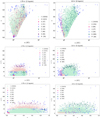 |
Fig. 4 Distributions of NEOs in different clusters in the spaces of eccentricity (e) vs. semi-major axis (a), inclination (i) vs. semi-major axis (a) and inclination (i) vs. eccentricity (e) for approach 1 (A1) at 1.78σ – left panel and approach 2 (A2) at 2σ – right panel. The legends correspond to different clusters with the numbers of NEOs in each of them. Cluster 0, illustrated by ‘+’ refers to the NEOs that are not included in any of the clusters by the G-mode. |
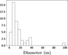 |
Fig. 5 Histograms with 5-meter binning showing the possible ranges of diameters derived for the NEOs in the C3 found for the G-mode run with approach 1 (A1) at q1 = 1.78. Except for two NEOs, for which albedos are available from literature (either assumed from their taxonomy or estimated from thermal emission), the albedos for other NEOs have been assumed to be a mean value of 0.147 following the works of Morbidelli et al. (2020). |
3.2 Approach 2 (A2)
3.2.1 A2 at q1 = 3
This approach (A2) includes six input variables as mentioned earlier and at the initial confidence level of 3σ, we find one homogeneous cluster of NEOs. The mean values of input variables and several ancillary parameters of interest are reported in Table A.6. The results indicate that more than 99% of the NEOs in our sample belong to one cluster, meaning that the entire sample of NEOs is homogeneous in terms of the six variables used at the confidence level of 3.0σ. The mean values of this cluster are comparable to the background population of NEOs (Table A.1). As was the case with the first approach (A1) at the confidence level of 3σ, the mean inclination and mean absolute magnitude remain the major discriminators between the homogeneous cluster of NEOs and the group of outlier NEOs.
3.2.2 A2 at q1 = 2.5
As we kept lowering q1, we noticed the emergence of a second cluster of NEOs (C2) at the confidence level of 2.5σ (Table A.7). From the sankey diagram of the Fig. 6, it is possible to notice that this second cluster gets seeded from the group of outlier NEOs with high inclination. The group of outlier NEOs resulted from this G-mode run have moderate inclinations with a mean ΤJ ~ 6.8 and are relatively smaller (mean H ~ 22.6).
3.2.3 A2 at q1 = 2.3
We observed the emergence of a third cluster of NEOs (C2) at the confidence level of 2.3σ (Table A.8) and this cluster corresponds to a cluster of smaller 47 NEOs (mean H ~ 29.4). This cluster is well-behaved in terms of the median absolute deviations of its orbital elements and ancillary parameters. We remark that a similar cluster (C3) of NEOs was found with the first approach (A1) at the confidence level of 1.78σ and NEOs in that cluster were slightly brighter or larger than this third cluster found using the second approach (A2). Despite the similar distributions in the orbital elements, the mean perihelia of these two clusters slightly differ from each other.
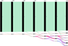 |
Fig. 6 Sankey diagram showing the transfer of objects among different clusters across G-mode runs of varying confidence levels from 3σ to 2σ. This diagram corresponds to the second approach where six input variables were used. The colours correspond to an Nth cluster in a given G-mode run, namely, the second cluster of any G-mode run will have the same colour. |
3.2.4 A2 at q1 = 2.2
A fourth cluster emerged at q1 = 2.2 and it corresponds to moderately inclined NEOs (mean of i ~ 16.5°) with relatively smaller semi-major axes (mean of a ~ 0.7 au), as reported in Table A.9. This characteristic distribution of orbital elements yields this cluster relatively higher TJ values (~7.8). It is also possible to notice that C2 (at q1 = 2.3) has now grown, almost doubling in size, thanks to the influx of NEOs from C1 and from the group of outliers at q1 = 2.3, as evident from the sankey diagram of Fig. 6.
3.2.5 A2 at q1 = 2.0
The clusters we obtained at q1 = 2.0 can be visualised with respect to e versus a, i versus a, and i versus e spaces in the right panel of Fig. 4. Their separation can best be visualised in the i versus a space – although C3, C4, and C5 are grouped together in this figure. Combining the information from the sankey diagram of Fig. 6 and from Table A.10, at q1 = 2.0, we notice that the latest cluster (C3 at q1 = 2.2) gets refined (including the removal of several outlier NEOs) as it gets sub-divided into three clusters with the main discriminator being the argument of perihelion ω. As reported in Table A.10, C3, C4, and C5 are only distinguishable by their mean ω values, which are also well behaved given their respective mean absolute deviations. In addition, we remark that previously found clusters remain stable and fed by an ongoing influx of NEOs, in spite of a confidence level that is consistently reduced, which makes a case for their stability.
We also highlight that C2 is stable and has grown in size with 194 NEOs at this confidence interval of 2.0σ. Its mean absolute magnitude of 28 implies that this cluster continues to contain relatively smaller NEOs. We made a histogram to visualise the estimated diameters of this cluster (Fig. 7). These estimations are closely comparable to the NEOs of cluster C3 resulted from A1 at 1.78σ (Fig. 5). It appears that both clusters sample a continuum of objects that are relatively small, characterised by a unimodal distribution peaking in the diameter range from 5 to 15 m. This can be further seen on Fig. 4, where they can be closely compared in the e versus a, i versus a, and i versus e spaces. We see that 36 out of 47 (>75%) NEOs in the cluster C3 resulted from A1 at 1.78σ find themselves in the cluster C2 resulted from A2 at 2.0σ, which reinforces the presence of a population of small NEOs with orbital elements that are similar to those of Arjuna-type asteroids (Tables A.5, A.10).
As for the C6, which represents NEOs of high inclination (mean i ~ 52°), it has grown in size compared to previous confidence level of 2.2σ. It proved that clusters began to lose their significance and become less meaningful if ql was further lowered below 2.0 for A2. Hence, we concluded the analysis for A2 at q1 = 2.0.
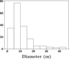 |
Fig. 7 Histograms with 5-m binning showing the possible ranges of diameters derived for the NEOs in the C2 found with the approach 2 (A2) at q1 = 2.0. Except for nine NEOs, for which albedos are available from literature (either assumed from their taxonomy or estimated from thermal emission), the albedos for other NEOs have been assumed to be a mean value of 0.147 following the works of Morbidelli et al. (2020). |
3.3 Potential escape regions for obtained G-mode NEO clusters
As reported up to now, our results are based on orbital and several ancillary NEO data applied to G-mode statistical tool and on available NEO taxonomical data. To expand on the dynamical aspect of this work, we probed potential source regions for NEO clusters resulted from our G-mode runs. Thus, we implemented an investigation similar to what was implemented by Binzel et al. (2019) to estimate a probability distribution for our G-mode clusters, taking into consideration a dynamical model of seven escape regions in the main asteroid belt. It is assumed that an object must escape from an escape region where it has held long-term residence dating back to the early Solar System, prior to entering the near-Earth space. This dynamical model (Granvik et al. 2016, 2017, 2018), the Granvik model hereafter, traces with scrutiny the escape paths of objects from the main-belt to near-Earth space and the model accounts for the Yarkovsky effect (Vokrouhlický et al. 2015). Given the orbital elements and absolute magnitude of an NEO, the Granvik model resolves a discrete probability distribution function, built up of seven values for following seven escape regions: (1) Hungaria asteroid family; (2) Phocaea asteroid family; (3) Resonance complex around ν6 secular resonance; (4) Resonance complex around 3:1 mean motion resonance with Jupiter; (5) Resonance complex around 5:2 mean motion resonance with Jupiter; (6) Resonance complex around 2:1 mean motion resonance with Jupiter; (7) JFCs.
As such, assuming that the NEOs belonging to a given cluster are represented by the mean values of the variables defining the cluster, we used the mean orbital elements and mean absolute magnitude of a cluster as inputs to the Granvik model (as if each cluster were a single NEO). For each approach, we selected the G-mode run with the largest number of clusters, as they represent more diversity, namely: clusters at 1.78σ for A1 and clusters at 2σ for A2 (Fig. 8).
As for approach 1 at 1.78σ, the results indicate that most of the clusters have higher probability to emanate via ν6 secular resonance, which is known to be the most dominant escape path from the main-belt to the near-Earth space (Bottke et al. 2002). In addition, we observe that C5 and C7 have significant probabilities to emanate from outer-belt sources, such as a 2:1 mean motion resonance of Jupiter and JFCs. These two clusters have been attributed to a primitive composition as we demonstrate earlier in this paper, based on their taxonomy and TJ, which are two independent pieces of evidence. Thus, our dynamic modeling reinforces and corroborates these existing results, pointing towards a primitive origin for the NEOs in these two classes. When it comes to approach 2, all the clusters obtained at 2σ have a greater probability of emanating via ν6 secular resonance, as expected (Bottke et al. 2002).
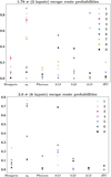 |
Fig. 8 Probability distributions for the G-mode clusters obtained at 1.78σ for A1 and at 2σ for A2 to emanate from any of the seven escape regions according to the Granvik model (Granvik et al. 2018). The numbers correspond to each of the clusters, represented by a unique colour. The group of outlier NEOs in each G-mode run is represented by the black colour represented by 0. The error bars correspond to the error of the mean for the nominal probability. |
4 Discussion
We implemented a G-mode analysis on NEOs structured on two distinct approaches based on input variables. During A1, we used i, e, and a of NEO orbits as inputs and during A2, we used six input variables which included i, e, a, TJ, H, and ω of NEOs.
With regard to A1, we started our G-mode analysis at a higher confidence level of 3σ and gradually lowered it down to 1.78σ. The most highly populated cluster emanating from the background population of NEOs was present in all the G-mode runs as it was the most dominating at all the confidence levels investigated. As far as A2 is concerned, we observed similar behaviour for the most highly populated cluster within the implemented confidence levels from 3.0σ to 2.0σ.
C6 obtained at the confidence level of 1.78σ with a mean 2 < TJ < 3 had a mixed composition (D and S-types) in terms of available taxonomy. Interestingly, Simion et al. (2021), in their work on spectral properties of NEOs with low TJ, report a particular group of 4 S-complex NEOs (e ≥ 0.92, q ≤ 0.3 au), which corresponds to some members of this C6. These authors propose that TJ ~ 3 can act as a compositional border transiting from non-primitive composition to a primitive composition and define the presence of S-type NEOs in highly eccentric orbits with low perihelia as an extreme case. Notably, they report (Table 6 in Simion et al. 2021) 394130 (2006 HY51), 465402 (2008 HW1), 455426 (2003 MT9), and 331471 (1984 QY1) as NEOs of this particular group and they are all members of our C6 in this G-mode run. Hence, we agree with the fact that TJ ~ 3 can indeed be used as a compositional border as proposed by the aforementioned authors. Our result also corroborates that the presence of S-complex NEOs in eccentric orbits in a regime of 2 < TJ < 3 is an extreme case. Having been given only three orbital parameters as inputs, G-mode not only initially finds NEOs corresponding to a cometary origin in terms of TJ at a higher confidence level, but also is able to independently find extreme compositionally heterogeneous sub-clusters (presence of S-type NEOs in a regime dominated by NEOs with primitive taxonomies (rich in organics and volatiles emanating from a cometary origin) inside the main cluster with a mean 2 < TJ < 3, at a lower confidence level. This is an important demonstration of the versatility of the G-mode method. As reported below Table A.5, we have 36 NEOs for which there is no available taxonomy in this C6. Based on the selection criterion of e ≥ 0.92, q ≤ 0.3 au, we report in Table A.11 the NEOs from C6, whose taxonomy is predicted to be of S-complex. We stress however, that the optical colors of 2002 PD43 published by Jewitt (2013) do not seem to match this prediction. Hence, more taxonomic data are needed to further verify the accuracy of this method.
We recall that DeMeo & Binzel (2008), based on spectroscopic data from a sample of 55 NEOs, estimated that 54 ± 10% of NEOs with TJ < 3 have comet-like spectra or albedos. Our clusters C5, C6 (excluding the extreme NEOs with S-type), and C7 in A1, associated with a primitive composition, capture about 21% of NEOs in our dataset with TJ < 3. Although the numbers are not close to each other, our estimate does not appear to be contradictory. In addition, Licandro et al. (2008) analyzed the spectra of asteroids with TJ < 3 also known as asteroids in cometary orbits (ACOs) and found that 35/41 of them contain featureless spectra with colours ranging from bluish to red (B-type to D-type), suggestive of a primitive composition. Then, Licandro et al. (2018) studied the spectra of 17 ACOs and 15 of them are of either D or X taxonomy, which also implies a primitive composition for these ACO, which these authors interpret as a strong signal for the presence of extinct or dormant comets. These findings are indeed comparable to the taxonomic distribution in C5, C6, and C7 in A1 (described earlier).
During A2, at the confidence level of 2.3σ we found a cluster (C2) of small NEOs whose stability and continuous growth were observed as the confidence level was decreased down to 2σ.
Given the mean orbital parameters and other reported ancillary parameters of this cluster, we highlight its close relationship with the C3 of A1 obtained at 1.78σ, thereby alluding to Arjuna-type asteroids. This cluster is more than four times more populous than C3, obtained during A1 at 1.78σ and shares more than three quarters of its NEOs with the former cluster. The estimated diameters of both clusters show unimodal distributions peaking in the range of 5–15 m (Figs. 5, 7). Although larger objects are more likely to be observed in general, the observed peak in the smaller dimensions does not necessarily discard the observational bias associated with this result as NEOs do not come close to the Earth at the same rate.
During A2, at the confidence level of 2.2σ, we obtained a fourth cluster of NEOs, characterised by a moderate mean inclination i ~ 16° and a mean semi-major axis of 0.7 au, which indicates that it is the cluster with the lowest orbital energy. Consequently, this cluster samples 25 of 37 known Atira asteroids. It is noteworthy that at the confidence level of 2.0σ, this cluster gets sub-divided into three new clusters, with a well-behaved argument of perihelion being the only discriminator. Although we do not find any evident significant taxonomical difference among the sub-divided clusters, they might hint towards a dynamical difference among themselves, given their well-separated and well-behaved arguments of perihelion.
We see that C8 and C6, obtained during A1 at q1 = 1.78σ and during A2 at q1 = 2.0σ, respectively, appear to share similar orbital elements and ancillary parameters. We compared the NEOs of each cluster individually and, indeed, we found that all the 88 NEOs of C8 obtained during A1 at q1 = 1.78σ are members of the C6 obtained during A2 at q1 = 2.0σ. Therefore, the latter appears to be an extension of the former. We note that the distributions of these two clusters in the i versus a and i versus e spaces in Fig. 4 also hint at this association.
As a general remark, we find that two clusters: (a) smaller NEOs with orbital parameters similar to those of Earth and (b) NEOs with relatively higher inclinations (i ~ 55°), are preserved during both approaches, without considering the background population, which is always represented as C1. Nevertheless, the clusters of NEOs associated with primitive composition during A1 are lost during A2. This is probably due to the inclusion of three additional variables during A2. Following the results obtained during A1, we propose that our method could potentially be used to make a reliable guess whether an NEO with an accurate enough orbital determination could be associated with a primitive taxonomy.
As a verification check on the obtained results, we performed several G-mode runs with different samples of NEOs selected by varying U. For example, we restricted the sample by U ≤ 4, U ≤ 3, U ≤ 2, and even U ≤ 6. Nevertheless, our G-mode runs with varying confidence levels resulted in groupings of clusters similar to those we had already obtained with U ≤ 5, as reported in this work. This provides verification that our results are independent of the method used for the NEO sample selection.
5 Conclusions
As a response to constrain the physical properties of NEOs, which are being discovered at an increasing rate, we attempted to find a way to make a reliable guess of the taxonomy of an NEO on the basis of its orbital elements. To achieve this, we used the G-mode clustering analysis. Our G-mode analysis of NEOs based on two approaches has led to the identification of unique clusters of NEOs. In each approach, we started at a confidence level of 3σ and gradually lowered it down to 1.78σ and 2σ for A1 and A2, respectively, allowing for more clusters to emerge. A1 allowed us to obtain clusters of NEOs that can be associated with a primitive composition based on their available taxonomy. The dynamical model we implemented to trace the escape regions of obtained G-mode clusters, strengthened this result, as it pointed towards outer-belt sources, correlated with a primitive origin. We also found a cluster of NEOs that can be associated with S-type NEOs in highly eccentric orbits with low perihelia which have been evoked in an earlier study and remarked on as an extreme case by Simion et al. (2021). Accordingly, we predicted (Table A.11) a list of NEOs that would be of an S-type taxonomy, waiting to be validated as soon as their taxonomic data are available.
We found two clusters that are common to both A1 and A2. The first of these is a cluster that samples small NEOs in orbits that are comparable to Earth’s orbit and that can be associated with Arjuna-type objects. The second of the shared clusters is the one with relatively high inclinations (i ~ 55°).
In terms of A2, we find three clusters that are only distinguishable by their arguments of perihelion. All of them have very low mean semi-major axes (0.7 au), moderate mean inclinations (i ~ 14°). Together, they comprise a sample of a majority of known Atira asteroids.
In synthesising the methods and results of this work, we propose that it is feasible to attempt to predict whether an NEO is of primitive taxonomy, provided that (1) its orbit is determined with a certain level of accuracy and (2) its orbital elements fall into the restricted combination regimes presented in Table 1.
Restricted combination regimes of NEO i, e, and a for which a reasonable guess for the taxonomy can be made.
Acknowledgements
We acknowledge the financial support from Agenzia Spaziale Italiana (ASI, contract no. 2017-37-H.0 CUP F82F17000630005). We also acknowledge funding from the European Union’s Horizon 2020 research and innovation programme under grant agreement no. 870403. This work has made use of the python astroquery library (Ginsburg et al. 2019).
Appendix A Statistics of G-mode results
Mean parameters of the population of NEOs and their median absolute deviations as of 27/10/2021.
G-mode clustering results for q1=3 (a confidence level of 3σ) with i, e, a as input parameters.
| C | N/A | A | B | C | D | K | L | O | Q | R | S | T | U | V | X |
|---|---|---|---|---|---|---|---|---|---|---|---|---|---|---|---|
| 1 | 12378 | 15 | 37 | 181 | 47 | 32 | 36 | 6 | 216 | 15 | 739 | 6 | 7 | 66 | 160 |
| 0 | 168 | 0 | 1 | 3 | 2 | 0 | 1 | 0 | 4 | 1 | 8 | 0 | 0 | 1 | 2 |
G-mode clustering results for q1=2.9 (a confidence level of 2.9σ) with i, e, a as input parameters.
| C | N/A | A | B | C | D | K | L | O | Q | R | S | T | U | V | X |
|---|---|---|---|---|---|---|---|---|---|---|---|---|---|---|---|
| 1 | 12348 | 15 | 36 | 181 | 47 | 32 | 36 | 6 | 216 | 15 | 737 | 6 | 7 | 64 | 160 |
| 2 | 183 | 0 | 2 | 3 | 1 | 0 | 1 | 0 | 4 | 1 | 10 | 0 | 0 | 3 | 2 |
| 0 | 15 | 0 | 0 | 0 | 1 | 0 | 0 | 0 | 0 | 0 | 0 | 0 | 0 | 0 | 0 |
G-mode clustering results for q1=1.9 (a confidence level of 1.9σ) with i, e, a as input parameters.
| C | N/A | A | B | C | D | K | L | O | Q | R | S | T | U | V | X |
|---|---|---|---|---|---|---|---|---|---|---|---|---|---|---|---|
| 1 | 11527 | 14 | 34 | 171 | 39 | 32 | 33 | 5 | 203 | 13 | 667 | 6 | 6 | 57 | 147 |
| 2 | 852 | 1 | 1 | 11 | 6 | 0 | 4 | 1 | 15 | 2 | 75 | 0 | 1 | 9 | 14 |
| 3 | 44 | 0 | 2 | 0 | 2 | 0 | 0 | 0 | 0 | 0 | 2 | 0 | 0 | 1 | 0 |
| 0 | 123 | 0 | 1 | 2 | 2 | 0 | 0 | 0 | 2 | 1 | 3 | 0 | 0 | 0 | 1 |
G-mode clustering results for q1=1.78 with i, e, a as input parameters.
| C | N/A | A | B | C | D | K | L | O | Q | R | S | T | U | V | X |
|---|---|---|---|---|---|---|---|---|---|---|---|---|---|---|---|
| 1 | 11157 | 14 | 32 | 159 | 36 | 32 | 33 | 5 | 196 | 13 | 643 | 6 | 6 | 56 | 144 |
| 2 | 1049 | 1 | 2 | 17 | 5 | 0 | 3 | 1 | 20 | 1 | 90 | 0 | 1 | 10 | 15 |
| 3 | 45 | 0 | 1 | 0 | 0 | 0 | 0 | 0 | 0 | 0 | 1 | 0 | 0 | 0 | 0 |
| 4 | 20 | 0 | 0 | 0 | 0 | 0 | 0 | 0 | 0 | 0 | 1 | 0 | 0 | 0 | 0 |
| 5 | 40 | 0 | 0 | 3 | 2 | 0 | 0 | 0 | 0 | 0 | 0 | 0 | 0 | 0 | 1 |
| 6 | 36 | 0 | 0 | 0 | 3 | 0 | 0 | 0 | 0 | 1 | 4 | 0 | 0 | 0 | 0 |
| 7 | 70 | 0 | 2 | 3 | 2 | 0 | 0 | 0 | 0 | 0 | 1 | 0 | 0 | 0 | 2 |
| 8 | 78 | 0 | 0 | 1 | 0 | 0 | 1 | 0 | 3 | 0 | 5 | 0 | 0 | 0 | 0 |
| 0 | 51 | 0 | 1 | 1 | 1 | 0 | 0 | 0 | 1 | 1 | 2 | 0 | 0 | 1 | 0 |
G-mode clustering results for q1=3.0 with i, e, a, ω, TJ and H as input parameters.
| C | N/A | A | B | C | D | K | L | O | Q | R | S | T | U | V | X |
|---|---|---|---|---|---|---|---|---|---|---|---|---|---|---|---|
| 1 | 12474 | 15 | 38 | 182 | 48 | 32 | 37 | 6 | 217 | 15 | 744 | 6 | 7 | 67 | 161 |
| 0 | 72 | 0 | 0 | 2 | 1 | 0 | 0 | 0 | 3 | 1 | 3 | 0 | 0 | 0 | 1 |
G-mode clustering results for q1=2.5 with i, e, a, ω, TJ and Has inputparameters.
| C | N/A | A | B | C | D | K | L | O | Q | R | S | T | U | V | X |
|---|---|---|---|---|---|---|---|---|---|---|---|---|---|---|---|
| 1 | 12377 | 15 | 37 | 182 | 47 | 32 | 35 | 6 | 216 | 14 | 732 | 6 | 7 | 64 | 160 |
| 2 | 106 | 0 | 1 | 2 | 0 | 0 | 1 | 0 | 3 | 2 | 9 | 0 | 0 | 2 | 2 |
| 0 | 63 | 0 | 0 | 0 | 2 | 0 | 1 | 0 | 1 | 0 | 6 | 0 | 0 | 1 | 0 |
G-mode clustering results for q1=2.3 with i, e, a, ω, TJ and Has inputparameters.
| C | N/A | A | B | C | D | K | L | O | Q | R | S | T | U | V | X |
|---|---|---|---|---|---|---|---|---|---|---|---|---|---|---|---|
| 1 | 12260 | 15 | 35 | 179 | 45 | 32 | 35 | 6 | 211 | 14 | 726 | 6 | 7 | 63 | 158 |
| 2 | 45 | 0 | 0 | 0 | 0 | 0 | 0 | 0 | 1 | 0 | 1 | 0 | 0 | 0 | 0 |
| 3 | 156 | 0 | 2 | 4 | 2 | 0 | 1 | 0 | 7 | 2 | 11 | 0 | 0 | 3 | 2 |
| 0 | 85 | 0 | 1 | 1 | 2 | 0 | 1 | 0 | 1 | 0 | 9 | 0 | 0 | 1 | 2 |
G-mode clustering results for q1=2.2 with i, e, a, ω, TJ and H as input parameters.
| C | N/A | A | B | C | D | K | L | O | Q | R | S | T | U | V | X |
|---|---|---|---|---|---|---|---|---|---|---|---|---|---|---|---|
| 1 | 12168 | 15 | 35 | 177 | 45 | 30 | 35 | 5 | 211 | 14 | 720 | 6 | 7 | 62 | 157 |
| 2 | 87 | 0 | 0 | 0 | 0 | 2 | 0 | 0 | 1 | 0 | 2 | 0 | 0 | 0 | 0 |
| 3 | 91 | 0 | 1 | 2 | 0 | 0 | 1 | 1 | 3 | 0 | 13 | 0 | 0 | 1 | 3 |
| 4 | 170 | 0 | 2 | 5 | 2 | 0 | 1 | 0 | 5 | 2 | 9 | 0 | 0 | 3 | 2 |
| 0 | 30 | 0 | 0 | 0 | 2 | 0 | 0 | 0 | 0 | 0 | 3 | 0 | 0 | 1 | 0 |
G-mode clustering results for q1=2.0 with i, e, a, ω, TJ, and H as input parameters.
| C | N/A | A | B | C | D | K | L | O | Q | R | S | T | U | V | X |
|---|---|---|---|---|---|---|---|---|---|---|---|---|---|---|---|
| 1 | 11930 | 15 | 32 | 173 | 44 | 30 | 35 | 5 | 209 | 13 | 701 | 6 | 6 | 61 | 150 |
| 2 | 185 | 0 | 1 | 1 | 1 | 2 | 0 | 0 | 1 | 0 | 2 | 0 | 0 | 0 | 1 |
| 3 | 55 | 0 | 1 | 1 | 0 | 0 | 0 | 0 | 1 | 0 | 6 | 0 | 0 | 1 | 3 |
| 4 | 35 | 0 | 1 | 0 | 0 | 0 | 0 | 0 | 1 | 1 | 8 | 0 | 0 | 0 | 1 |
| 5 | 46 | 0 | 0 | 1 | 0 | 0 | 1 | 1 | 1 | 0 | 7 | 0 | 0 | 0 | 2 |
| 6 | 238 | 0 | 2 | 8 | 2 | 0 | 1 | 0 | 6 | 2 | 17 | 0 | 1 | 4 | 5 |
| 0 | 57 | 0 | 1 | 0 | 2 | 0 | 0 | 0 | 1 | 0 | 6 | 0 | 0 | 1 | 0 |
NEOs predicted to be associated with an S-complex taxonomy from the analysis of this work and the results of Simion et al. (2021).
References
- Altwegg, K., Balsiger, H., Bar-Nun, A., et al. 2015, Science, 347 [Google Scholar]
- Barucci, M., Capria, M., Coradini, A., & Fulchignoni, M. 1987, Icarus, 72, 304 [NASA ADS] [CrossRef] [Google Scholar]
- Barucci, M. A., Belskaya, I. N., Fulchignoni, M., & Birlan, M. 2005, AJ, 130, 1291 [CrossRef] [Google Scholar]
- Barucci, M. A., Hasselmann, P. H., Fulchignoni, M., et al. 2019, A & A, 629, A13 [CrossRef] [EDP Sciences] [Google Scholar]
- Binzel, R. P., DeMeo, F. E., Turtelboom, E. V., et al. 2019, Icarus, 324, 41 [Google Scholar]
- Bott, N., Perna, D., Deshapriya, J. D. P., et al. 2022, Planet. Space Sci., 219, 105530 [NASA ADS] [CrossRef] [Google Scholar]
- Bottke, W. F., Morbidelli, A., Jedicke, R., et al. 2002, Icarus, 156, 399 [NASA ADS] [CrossRef] [Google Scholar]
- Brown, P. G., Assink, J. D., Astiz, L., et al. 2013, Nature, 503, 238 [NASA ADS] [Google Scholar]
- Bus, S. J., & Binzel, R. P. 2002, Icarus, 158, 146 [Google Scholar]
- Carruba, V., De Oliveira, E. R., Rodrigues, B., & Requena, I. 2018, MNRAS, 479, 4815 [NASA ADS] [CrossRef] [Google Scholar]
- de la Fuente Marcos, C. & de la Fuente Marcos, R. 2015, Astron. Nachr., 336, 5 [Google Scholar]
- DeMeo, F., & Binzel, R. P. 2008, Icarus, 194, 436 [NASA ADS] [CrossRef] [Google Scholar]
- DeMeo, F. E., Binzel, R. P., Slivan, S. M., & Bus, S. J. 2009, Icarus, 202, 160 [Google Scholar]
- DeMeo, F. E., Alexander, C. M. O., Walsh, K. J., Chapman, C. R., & Binzel, R. P. 2015, The Compositional Structure of the Asteroid Belt, eds. P. Michel, F. E. DeMeo, & W. F. Bottke, 13 [Google Scholar]
- Devogèle, M., Moskovitz, N., Thirouin, A., et al. 2019, AJ, 158, 196 [CrossRef] [Google Scholar]
- Di Ruzza, S., Pousse, A., & Alessi, E. M. 2023, Icarus, 390, 115330 [NASA ADS] [CrossRef] [Google Scholar]
- Ehrenfreund, P., & Sephton, M. A. 2006, Faraday Discuss., 133, 277 [NASA ADS] [CrossRef] [Google Scholar]
- Fatka, P., Moskovitz, N. A., Pravec, P., et al. 2022, MNRAS, 510, 6033 [NASA ADS] [CrossRef] [Google Scholar]
- Gavrishin, A. I., Coradini, A., & Cerroni, P. 1992, Earth Moon Planets, 59, 141 [NASA ADS] [CrossRef] [Google Scholar]
- Ginsburg, A., Sipőcz, B. M., Brasseur, C. E., et al. 2019, AJ, 157, 98 [Google Scholar]
- Granvik, M., Morbidelli, A., Jedicke, R., et al. 2016, Nature, 530, 303 [Google Scholar]
- Granvik, M., Morbidelli, A., Vokrouhlický, D., et al. 2017, A & A, 598, A52 [NASA ADS] [CrossRef] [EDP Sciences] [Google Scholar]
- Granvik, M., Morbidelli, A., Jedicke, R., et al. 2018, Icarus, 312, 181 [CrossRef] [Google Scholar]
- Hasselmann, P. H., Carvano, J. M., & Lazzaro, D. 2013, AA (Observatório Nacional, MCTI-Brazil), AB(Observatório Nacional, MCTI-Brazil), AC(Observatório Nacional, MCTI-Brazil), 48 [Google Scholar]
- Hromakina, T., Birlan, M., Barucci, M. A., et al. 2021, A & A, 656, A89 [NASA ADS] [CrossRef] [EDP Sciences] [Google Scholar]
- Ieva, S., Dotto, E., Mazzotta Epifani, E., et al. 2020, A & A, 644, A23 [NASA ADS] [CrossRef] [EDP Sciences] [Google Scholar]
- Jedicke, R., Granvik, M., Micheli, M., et al. 2015, Surveys, Astrometric Follow-Up, and Population Statistics, 795 [Google Scholar]
- Jewitt, D. 2005, AJ, 129, 530 [NASA ADS] [CrossRef] [Google Scholar]
- Jewitt, D. 2013, AJ, 145, 133 [NASA ADS] [CrossRef] [Google Scholar]
- Licandro, J., Alvarez-Candal, A., de León, J., et al. 2008, A & A, 481, 861 [NASA ADS] [CrossRef] [EDP Sciences] [Google Scholar]
- Licandro, J., Popescu, M., de León, J., et al. 2018, A & A, 618, A170 [NASA ADS] [CrossRef] [EDP Sciences] [Google Scholar]
- Lin, C.-H., Ip, W.-H., Lin, Z.-Y., et al. 2018, Planet. Space Sci., 152, 116 [NASA ADS] [CrossRef] [Google Scholar]
- Mainzer, A. K., Bauer, J. M., Cutri, R. M., et al. 2019, NASA Planetary Data System [Google Scholar]
- Marty, B., Avice, G., Sano, Y., et al. 2016, Earth Planet. Sci. Lett., 441, 91 [CrossRef] [Google Scholar]
- Mommert, M., Hora, J. L., Harris, A. W., et al. 2014, ApJ, 781, 25 [NASA ADS] [CrossRef] [Google Scholar]
- Morbidelli, A., & Vokrouhlický, D. 2003, Icarus, 163, 120 [NASA ADS] [CrossRef] [Google Scholar]
- Morbidelli, A., Delbo, M., Granvik, M., et al. 2020, Icarus, 340, 113631 [NASA ADS] [CrossRef] [Google Scholar]
- Perna, D., Barucci, M. A., & Fulchignoni, M. 2013, A & ARv, 21, 65 [Google Scholar]
- Perna, D., Fulchignoni, M., Barucci, M. A., et al. 2017, A & A, 600, A115 [CrossRef] [EDP Sciences] [Google Scholar]
- Perna, D., Barucci, M. A., Fulchignoni, M., et al. 2018, Planet. Space Sci., 157, 82 [CrossRef] [Google Scholar]
- Popova, P. O., Peter, J., Vacheslav, E., et al. 2013, Science, 342, 1069 [NASA ADS] [CrossRef] [Google Scholar]
- Pravec, P., & Harris, A. W. 2007, Icarus, 190, 250 [CrossRef] [Google Scholar]
- Simion, N. G., Popescu, M., Licandro, J., et al. 2021, MNRAS, 508, 1128 [NASA ADS] [CrossRef] [Google Scholar]
- Sosa, A., Fernández, J. A., & Pais, P. 2012, A & A, 548, A64 [NASA ADS] [CrossRef] [EDP Sciences] [Google Scholar]
- Tosi, F., Coradini, A., Gavrishin, A. I., et al. 2005, Earth Moon Planets, 96, 165 [Google Scholar]
- Vokrouhlický, D., Bottke, W. F., Chesley, S. R., Scheeres, D. J., & Statler, T. S. 2015, in Asteroids IV, 509 [Google Scholar]
All Tables
Restricted combination regimes of NEO i, e, and a for which a reasonable guess for the taxonomy can be made.
Mean parameters of the population of NEOs and their median absolute deviations as of 27/10/2021.
G-mode clustering results for q1=3 (a confidence level of 3σ) with i, e, a as input parameters.
G-mode clustering results for q1=2.9 (a confidence level of 2.9σ) with i, e, a as input parameters.
G-mode clustering results for q1=1.9 (a confidence level of 1.9σ) with i, e, a as input parameters.
G-mode clustering results for q1=3.0 with i, e, a, ω, TJ and H as input parameters.
G-mode clustering results for q1=2.5 with i, e, a, ω, TJ and Has inputparameters.
G-mode clustering results for q1=2.3 with i, e, a, ω, TJ and Has inputparameters.
G-mode clustering results for q1=2.2 with i, e, a, ω, TJ and H as input parameters.
G-mode clustering results for q1=2.0 with i, e, a, ω, TJ, and H as input parameters.
NEOs predicted to be associated with an S-complex taxonomy from the analysis of this work and the results of Simion et al. (2021).
All Figures
|
Fig. 1 Distribution of NEOs belonging to dynamical groups Atiras. Atens, Apollos, and Amors, included in this work. |
| In the text | |
|
Fig. 2 Taxonomic distribution of NEOs included in this work. The x-axis refers to different taxonomic types and N/A corresponds to NEOs for which taxonomic data are not currently available. |
| In the text | |
|
Fig. 3 Sankey diagram showing the transfer of objects among different clusters across G-mode runs of varying confidence levels from 3σ to 1.78σ. This diagram corresponds to the first approach where three input variables were used. The colours correspond to an Nth cluster in a given G-mode run, i.e. the second cluster of any G-mode run will have the same colour. |
| In the text | |
|
Fig. 4 Distributions of NEOs in different clusters in the spaces of eccentricity (e) vs. semi-major axis (a), inclination (i) vs. semi-major axis (a) and inclination (i) vs. eccentricity (e) for approach 1 (A1) at 1.78σ – left panel and approach 2 (A2) at 2σ – right panel. The legends correspond to different clusters with the numbers of NEOs in each of them. Cluster 0, illustrated by ‘+’ refers to the NEOs that are not included in any of the clusters by the G-mode. |
| In the text | |
|
Fig. 5 Histograms with 5-meter binning showing the possible ranges of diameters derived for the NEOs in the C3 found for the G-mode run with approach 1 (A1) at q1 = 1.78. Except for two NEOs, for which albedos are available from literature (either assumed from their taxonomy or estimated from thermal emission), the albedos for other NEOs have been assumed to be a mean value of 0.147 following the works of Morbidelli et al. (2020). |
| In the text | |
|
Fig. 6 Sankey diagram showing the transfer of objects among different clusters across G-mode runs of varying confidence levels from 3σ to 2σ. This diagram corresponds to the second approach where six input variables were used. The colours correspond to an Nth cluster in a given G-mode run, namely, the second cluster of any G-mode run will have the same colour. |
| In the text | |
|
Fig. 7 Histograms with 5-m binning showing the possible ranges of diameters derived for the NEOs in the C2 found with the approach 2 (A2) at q1 = 2.0. Except for nine NEOs, for which albedos are available from literature (either assumed from their taxonomy or estimated from thermal emission), the albedos for other NEOs have been assumed to be a mean value of 0.147 following the works of Morbidelli et al. (2020). |
| In the text | |
|
Fig. 8 Probability distributions for the G-mode clusters obtained at 1.78σ for A1 and at 2σ for A2 to emanate from any of the seven escape regions according to the Granvik model (Granvik et al. 2018). The numbers correspond to each of the clusters, represented by a unique colour. The group of outlier NEOs in each G-mode run is represented by the black colour represented by 0. The error bars correspond to the error of the mean for the nominal probability. |
| In the text | |
Current usage metrics show cumulative count of Article Views (full-text article views including HTML views, PDF and ePub downloads, according to the available data) and Abstracts Views on Vision4Press platform.
Data correspond to usage on the plateform after 2015. The current usage metrics is available 48-96 hours after online publication and is updated daily on week days.
Initial download of the metrics may take a while.