| Issue |
A&A
Volume 672, April 2023
|
|
|---|---|---|
| Article Number | A188 | |
| Number of page(s) | 10 | |
| Section | Stellar structure and evolution | |
| DOI | https://doi.org/10.1051/0004-6361/202345966 | |
| Published online | 21 April 2023 | |
Serendipitous discovery of the magnetic cataclysmic variable SRGE J075818−612027
1
Leibniz-Institut für Astrophysik Potsdam (AIP), An der Sternwarte 16, 14482 Potsdam, Germany
e-mail: This email address is being protected from spambots. You need JavaScript enabled to view it.
2
Department of Astronomy & Space Sciences, Faculty of Science, University of Ege, 35100 Bornova, Izmir, Turkey
3
South African Astronomical Observatory, PO Box 9 Observatory Road, Observatory, 7935 Cape Town, South Africa
4
Department of Astronomy, University of Cape Town, Private Bag X3, Rondebosch 7701, South Africa
5
Department of Physics, University of the Free State, PO Box 339 Bloemfontein 9300, South Africa
Received:
20
January
2023
Accepted:
24
February
2023
Abstract
We report the discovery of SRGE J075818−612027, a deep stream-eclipsing magnetic cataclysmic variable found serendipitously in SRG/eROSITA calibration and performance verification phase (CalPV) observations of the open cluster NGC 2516 as an unrelated X-ray source. An X-ray timing and spectral analysis of the eROSITA data is presented and supplemented by an analysis of TESS photometry and SALT spectroscopy. X-ray photometry reveals two pronounced dips repeating with a period of 106.144(1) min. The 14-month TESS data reveal the same unique period. A low-resolution identification spectrum obtained with SALT displays hydrogen Balmer emission lines on a fairly blue continuum. The spectrum and the stability of the photometric signal led to the classification of the new object as a polar-type cataclysmic variable. In this context, the dips in the X-ray light curve are explained by absorption in the intervening accretion stream and by a self-eclipse of the main accretion region. The object displays large magnitude differences on long timescales (months) both at optical and X-ray wavelengths, which are interpreted as high and low states and thus support its identification as a polar. The bright phase X-ray spectrum can be reflected with single temperature thermal emission with 9.7 keV and bolometric X-ray luminosity LX ≃ 8 × 1032 erg s−1 at a distance of about 2.7 kpc. The X-ray spectrum lacks the pronounced soft X-ray emission component prominently found in ROSAT-discovered polars.
Key words: novae / cataclysmic variables / binaries: close / X-rays: binaries / stars: individual: SRGE J075818−612027 / stars: fundamental parameters
© The Authors 2023
 Open Access article, published by EDP Sciences, under the terms of the Creative Commons Attribution License (https://creativecommons.org/licenses/by/4.0), which permits unrestricted use, distribution, and reproduction in any medium, provided the original work is properly cited.
This article is published in open access under the Subscribe to Open model. This email address is being protected from spambots. You need JavaScript enabled to view it. to support open access publication.
1. Introduction
The AM Her systems, or polars, are interacting close binaries that consist of an accreting white dwarf (WD; called the primary) and a Roche-lobe filling donor star (often referred to as the secondary) typically on the main sequence. The objects are magnetic cataclysmic binaries or cataclysmic variables (CVs). Hence, interaction takes place via Roche-lobe overflow to the WD. The WDs in these systems have strong magnetic fields, B > 10 MG, that keep both stars in synchronous rotation, suppress formation of an accretion disk, and guide accreted matter to the polar regions of the WD where its potential energy is ultimately released through radiation from the cooling-shocked plasma at X-ray wavelengths and via cyclotron radiation at optical and neighboring wavelength regimes (Warner 1995).
Polars have been found as soft X-ray emitters with the Einstein satellite and with the Röntgensatellit (ROSAT). Soft X-ray emission of reprocessed origin or from deeply buried filamentary accretion shocks (Lamb & Masters 1979; Frank et al. 1988) was regarded as one of the observational hallmarks of the class.
Interestingly, the polar survey conducted by Ramsay & Cropper (2004) with the X-ray Multi-Mirror Mission (XMM-Newton) and all serendipitous discoveries made with XMM-Newton since then (Vogel et al. 2008; Ramsay et al. 2009; Webb et al. 2018; Schwope et al. 2020) have not revealed any further evidence for soft X-ray emission from a large number of magnetic CVs. Also, the first eROSITA-discovered polar did not show pronounced soft X-ray emission (Schwope et al. 2022). Meanwhile, about 150 magnetic CVs are known that belong to the polar subclass of the CV population (Ritter & Kolb 2003).
Polars are in the last steps of binary star evolution and typically have short orbital periods (Porb < 2 h) (Ritter & Kolb 2003; Knigge 2006). Magnetic torques keep the spin of the WDs synchronized with the orbit so that for most polars Porbit = Pspin. Accordingly, accretion-related emission is modulated on this period. Polars may show alternating high and low accretion states due to cessation of the mass flow from the donor to the WD. Such accretion rate changes are thought to be related to the magnetic activity of the secondary star (Livio & Pringle 1994). The optical brightness of the prototype polar, AM Herculis, which has more than a century of optical observations, differs by 2.5 mag between high and low states (Hessman et al. 2000; Wu & Kiss 2008; Schwope et al. 2020).
The extended Roentgen Survey utilizing an Imaging Telescope Array (eROSITA) instrument (Predehl et al. 2021) on board the Spektrum-Roentgen-Gamma spacecraft (Sunyaev et al. 2021) was launched in July 2019 and brought into a wide halo orbit around the Sun–Earth L2 point. Its main aim is to perform several X-ray all-sky surveys (called eRASS), each lasting six months, in the energy range of 0.2 − 10 keV.
Prior to the main survey, a comprehensive calibration and performance verification (CalPV) phase of the mission took place. During this phase, the galactic open cluster NGC 2516 (also known as Caldwell 96) was observed in order to calibrate the boresight and plate scale. The analysis of the data on the cluster member stars will be reported in Fritzewski et al. (in prep.). In this paper, we report on the serendipitous discovery of a new magnetic cataclysmic variable in the field of NGC 2516, SRGE J075818−612027 (hereafter SRGE0758). The object could be identified initially based on its regular variability pattern, which became obvious through visual inspection of the data cube made from the distribution of events in the space spanned by the x, y, and time coordinates. The object was also reported as variable in the Gaia DR3 catalog, with a variability flag that indicates long-term photometric variations (see Eyer et al. 2023, and references therein).
We detail the X-ray observations obtained by eROSITA with the comprehensive photometric Transiting Exoplanet Survey Satellite (TESS) data and descriptive spectral observation in Sect. 2. We present the basic features of the system based on the results of considering the X-ray and optical data together in Sect. 3. In Sect. 4, we discuss our recent results.
2. Observations
2.1. Discovery with eROSITA
Aboard eROSITA are seven identical cameras (TM1-TM7) covering the same field of view with approximately 1 deg diameter. The X-ray observations of NGC 2516 occurred on October 5, 2019 (OBS ID 700018, 60.6 ks good time), and October 31, 2019 (OBS ID 700019, 80 ks good time), in pointed mode. Observation 700018 was carried out with only three cameras (TM5, TM6, and TM7), while 700019 was carried out with all seven cameras.
The data were reduced with the eROSITA Science Analysis Software System (eSASS) version eSASSusers_211214 (Brunner et al. 2022). In order to determine the remaining astrometric offsets between the two data sets, both observations were astrometrically calibrated. Preliminary eSASS source lists were generated for both observations, and corresponding Gaia counterparts were assigned within a 12 arcsec matching radius. Finding the optimal 3D rotation matrix Ropt needed to minimize the differences between the X-ray positions and Gaia reference positions resembled Wahba’s problem (Wahba 1965). To resolve the problem, we applied a method described in Markley & Crassidis (2014) using the singular value decomposition to find Ropt.
For each of the two observations, the matrix Ropt defines an offset in the equatorial coordinates α, δ, and in the roll angle ϕ. Neglecting the small roll angle correction, we applied the following corrections to each event:

with Δα = −2.087 arcsec, Δδ = +0.052 arcsec for observation 700018, and Δα = −2.835 arcsec, Δδ = +4.685 arcsec for observation 700019.
The corrected event lists were then merged, and a stacked image in the 0.2–5.0 keV energy band was created (see Fig. 1). The new object we report, SRGE0758, was one of the brightest X-ray sources in the field of NGC 2516 (see Fig. 1).
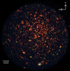 |
Fig. 1. X-ray image of the NGC 2516 obtained by eROSITA. The white dashed circle marks the position of SRGE0758. False colors of the image were made using photon energies between 0.2 and 1.1 keV, 1.1 and 2.3 keV, and 2.3 and 5 keV for the red, green, and blue channels, respectively. The image displays an area of 1×1 deg. |
2.2. Gaia observations
In Gaia DR3 (Gaia Collaboration 2021), SRGE0758 is referred to as ID 5290647986316685824 with the sky coordinates Dec2000 = 119.57648825065 deg and RA2000 =−61.34105844684 deg. The mean brightness of the object is 19.73 ± 0.03, 19.90 ± 0.13, and 18.96 ± 0.09 in the G, GBP, and GRP passbands, respectively. We used the geometric Gaia distance (rgeo) to the system of  pc, as determined by Bailer-Jones et al. (2021b). The photometric distance (rpgeo) is unreliable at G > 19 mag according to Creevey et al. (2023) and Fouesneau et al. (2023). The sky position of the source is shown in Fig. 2.
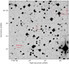 |
Fig. 2. DSS image of the sky region around SRGE0758. The optical counterpart is marked with red lines. |
2.3. TESS observations
The TESS satellite provides high time precision light curves for time domain astrophysics (Ricker et al. 2014). The satellite is equipped with four identical refractive cameras and observes the sky in sectors with 24 × 96 deg. Each sector is observed for two orbits of the satellite around the Earth, or about 27 days on average. Each of the 2k × 2k charge couple devices (CCDs) on the satellite has a scale of 21 arcsec per pixel.
Observations of SRGE0758 occurred in seven TESS sectors. The sector IDs of these observations are 27, 28, 31, 34, 35, 36, and 37. These observations can be accessed from the Mikulski Archive for Space Telescopes1. The observations were made between July 5, 2020, and April 2, 2021, about one year after the eROSITA observations, and were carried out with a time resolution of 475 s.
We extracted the photometry from the TESS full-frame images using eleanor (Feinstein et al. 2019), which allowed us to obtain a cutout of the 31 × 31 pixel postcard of the calibrated full-frame images centered on the target source. The eleanor tool removes the background, corrects for systematic errors, and derives a light curve for different apertures.
All sectors were reduced to 11 × 11 pixel subgrids. We used the default pixel source extraction area that was produced by eleanor for the source to obtain the time series. For each sector, we plotted Gaia DR3 measurements over the field and checked the correct extraction location for the source.
During the extraction process, we encountered two relevant challenges: (1) At G≃19.7 the source is very faint, almost at background level. In some sectors, this characteristic indeed led to background-subtracted light curves with negative fluxes. (2) Gaia data have shown that a neighboring source falls into the same TESS pixel. This object is ∼8 arcsec away from our target, with coordinates RA1 = 119.57869730126448 and Dec1 = −61.34270664883291 (source ID 5290647917596586112, G = 19.71 ± 0.02 mag). We checked the variability of this neighboring source from Gaia DR3. Importantly, the new Gaia DR3 catalog was released with a variability column (Eyer et al. 2023), and noted in this column is whether the system is a variable from long-term photometry. There was no indication about the brightness variability of the contaminating source. All this means that the already weak signal from our target is further diluted by the signal from the neighboring star so that neither absolute brightness values nor absolute variability amplitudes can be determined.
Given these extra challenges, we performed a variability analysis on normalized light curves. To investigate possible periodic variations in all sectors, we applied a Savitzky-Golay smoothing filter algorithm with the “flatten” task in “lightkurve” software (Lightkurve Collaboration 2018). The data obtained in one of the sectors (sector 35) are shown in Fig. 3.
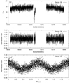 |
Fig. 3. TESS light curve of SRGE0758 obtained for sector 35. Panel (a): background corrected TESS light curve in original time series. Panel (b): normalized light curve for sector 35. Panel (c): folded light curve of sector 35 according to Eq. (1) in normalized flux. |
2.4. Follow-up spectroscopy with SALT
We carried out optical spectroscopic observations of the object with the 11-m Southern African Large Telescope (SALT) at Sutherland Observatory (Buckley et al. 2006). The 1200 s exposure was performed with the Robert Stobie Spectrograph (Burgh et al. 2003) on May 24, 2022. The grism (pg0300) covers 4000–8000 Å with a small gap at 4900–5100 Å. The grism together with the used slit width of 1 5 resulted in a spectral resolution of 17 Å at the full width at half maximum (FWHM). The spectrophotometric standard star Feige 110 (Oke 1990), observed with SALT on May 15, 2022, was used for the flux calibration. The calibration was done through Image Reduction and Analysis Facility (IRAF) software (Tody 1986) by fitting a spline3 function to the observed spectrum of the standard to determine the sensitivity function, which was then applied to the spectrum of SRGE0758. We could only obtain relative flux calibrations from observing a spectrophotometric standard in twilight due to the nature of the SALT design and the moving entrance pupil (Buckley et al. 2018).
3. Analysis and results
3.1. Optical photometry from TESS
To find any periodic changes in the optical light curve, we used the Lomb and Scargle periodogram, which is useful in non-sinusoidal time series (Lomb 1976; Scargle 1982; VanderPlas 2018). We searched for significant peaks in the frequency interval from 0 d−1 up to the Nyquist frequency in TESS data (182 d−1). The resulting power spectrum showed a main peak at P = 106 min.
Following Baluev (2008), we computed the false alarm probability to check the significance of the peak. The false alarm probability was zero, confirming that the main peak belongs to a real periodic variation. We measured the uncertainty of this period with a Gaussian fit applied to the periodogram peak. At 95% confidence, the uncertainty is  , so the final TESS-period is
  .
.
We applied the same method to the eROSITA X-ray light curve obtained in the 0.2 − 2.3 keV band. The resulting periodogram also showed a peak at P = 0.0738(5) (106.2(7) min), fully compatible with the TESS period, so we find coherent periodic variations of both the optical and X-ray light curves at 106 min. The power spectrum of both light curves is displayed in the Fig. 4. No other periodicity was found in the power spectrum, except for the harmonics of the main peak.
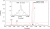 |
Fig. 4. Lomb-Scargle periodogram of the TESS and eROSITA observations. The main figure shows the over plotted power spectra of the object obtained from TESS and eROSITA, and the inset details the main peak of the TESS observations. The dashed black line shows a Gaussian line fit to the main peak. The red dashed line in the main frame gives the 99% significance level of the eROSITA power spectrum. The main period and its harmonics are indicated with the Ω symbol. The horizontal black dashed line within the inset indicates the 99% significance level for the TESS spectrum. |
In the bottom panel of Fig. 3, we show the folded TESS light curve. The original data were initially phase folded with an arbitrary time of zero. The resulting signal showed a roughly sinusoidal brightness variation in all sectors (around ∼5000 photometric cycles). The (arbitrary) phase of maximum brightness was determined with a Gaussian fit, and the zero time was corrected accordingly so that our final ephemeris for the folding of data and the determination of the TESS maximum brightness reads as
 (1)
(1)
where the numbers in parentheses give the uncertainties in the last digits. In the following sections, all phases refer to the ephemeris given in Eq. (1).
In all sectors, TESS light curves always show the same sinusoidal brightness variation, but the amplitude of the sine curve changes considerably. We are working against limits of the instrument due to the relatively faint nature of the object. Therefore, the variable amplitude is due to the subtraction of different background levels sector to sector. It is not possible to make an inference on the long-term variation of the object with TESS, but regarding the short-term variation, we obtained a very strong signal that gives the same photometric period as the X-ray data in all sectors, and this result is quite consistent.
3.2. SALT spectroscopy
In Fig. 5, the SALT spectrum is shown. The object displays several hydrogen Balmer emission lines superposed on a flat continuum. Other lines were tentatively detected (HeI5875, OI6300, and HeII4686), but closer inspection of the raw and sky-subtracted 2D spectra showed that these lines were possibly duplicated by cosmic ray hits on the CCD. We consider the information obtained from these lines as unreliable and ignored them in our further analysis. The lines are indicated by the gray bars in Fig. 5.
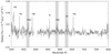 |
Fig. 5. SALT spectrum of the SRGE0758. The wavelength ranges strongly contaminated by sky lines or cosmic rays are indicated in gray. |
To determine the parameters of the hydrogen Balmer lines, the continuum was approximated with a low-order polynomial, and the spectrum was normalized to this continuum. Line parameters were determined by single Gaussians fits to the data. The fitted emission lines are listed in Table 1. The signal-noise ratio is low at the blue end of the spectrum, and the measurement of the Hδ line in particular is rather uncertain. Different from the other lines, the Hδ line has a double-peaked shape, which is regarded as being apparent only. Its measurements are regarded as controversial (indicated by a colon in Table 1).
Spectral parameters of Balmer emission lines in the SALT spectrum.
From the flat continuum at 6250 Å, the mean spectral flux density is about 6.5 × 10⁻¹⁸ erg cm−2 s−1 Å−1, which corresponds to a GaiaG-band magnitude of 21.5 (Vega). Hence, at the time when the spectrum was obtained, the source appeared considerably fainter than previously found with Gaia (G ∼ 19.7 mag). The spectral exposure was started at JD 2459724.2284838, so the spectrum thus covered the phase interval of 0.07 − 0.26, which corresponds to the decreasing branch of the TESS light curve.
Strong emission lines of hydrogen and helium, both neutral and ionized, are the main indicators for identifying a source as a CV (Szkody et al. 1998). We have only discovered hydrogen Balmer emission lines with certainty. This feature and the low brightness at the time of the SALT observation is indicative of the object having a low accretion state during our observations. Low accretion states are regularly found in strongly magnetic CVs (i.e., polars). In these states, typically only hydrogen Balmer lines (in particular Hα) are visible (Schwope et al. 2002). The SALT spectroscopy thus suggests SRGE0758 is a polar in a low accretion state.
3.3. eROSITA observations
3.3.1. X-ray photometry
The eROSITA X-ray light curves of both observations of SRGE0758 are shown in original time sequence in Fig. 6. Only data in the interval 0.2 − 2.3 keV and time bins of 100 s were used for light curves. The object showed pronounced brightness variations, with one bright hump and two dips or eclipse-like brightness minima. While the main minimum can always be clearly recognized, the second one following in time is quite shallow. This overall variability pattern is visible during all 22 cycles that were covered during the X-ray observations. The main minimum sometimes has a zero count rate but remains finite at other instances. Hence, the main minimum is not interpreted as a true eclipse, as the count rate in such a case would always be consistent with zero.
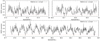 |
Fig. 6. eROSITA 0.2 − 2.3 keV X-ray light curve of SRGE0758 with time bins of 100 s. The top row shows the data from ObsID 700018 and the lower row shows that of ObsID 700019. |
We generated energy-resolved and phase-folded X-ray light curves in two energy bands: a soft band between 0.2 and 0.8 keV and a hard band between 0.8 and 2.3 keV. These are shown in Figs. 7b and c. The first dip is located at phase 0.40 and has a FWHM of 0.07 phase units. The flux is almost zero in the soft band (0.2 − 0.8 keV), but it is always positive in the hard band (0.8 − 2.3 keV). The second dip shows a contrasting behavior. The dip is centered on phase 0.69, that is, 0.29 phase units after the first one. It is shallow in soft X-ray band and more pronounced and deeper in the hard band.
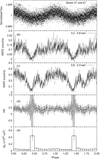 |
Fig. 7. TESS, energy-resolved eROSITA light curves, HR and NH variations of SRGE0758 for ObsID 700019. Panel (a): TESS light curve obtained from sectors 31 and 37. Panels (b) and (c): X-ray data in the two indicated energy bands originally binned using 50 s time bins and averaged using a phase bin size of 0.005 phase units. Panel (d): HR obtained from 0.2 to 0.8 keV and 0.8 to 2.3 keV energy bands. Panel (e): column density variation. All light curves folded according to photometric period and T0, max in Eq. (1). |
To gain a better understanding of these variations, we calculated the hardness ratio (HR) between the two chosen bands. The HR was defined as HR = (H − S)/(H + S), and thus it can vary between −1 and +1 for supersoft and superhard sources (see Fig. 7d). Outside the dips, the HR shows little variability and scatters around the 0.5 phase.
The dips (or eclipse-like features) could be related to photo-electric absorption or to geometric effects such as self-eclipses and/or geometric foreshortening of the corresponding emission regions. The observed spectral hardening during the first dip implies that it is likely caused by photo-electric absorption. The absorber is the magnetically guided stream or curtain out of the orbital plane, as studied by Watson et al. (1989) and described by Kuulkers et al. (2010). The energy-independent variation during the second dip suggests that it is more likely caused by foreshortening and/or self-eclipsing of the accretion and/or emission region(s) as the WD rotates. The self-eclipse is not total but only partial, which can be explained if the emission region is extended and does not completely vanish behind the limb of the WD as it rotates.
3.3.2. X-ray spectroscopy
Spectral analysis was performed with the XSPEC package (version 12.12.0; Arnaud 1996; Dorman & Arnaud 2001). Only photons between 0.2 and 5 keV were included in the spectral analysis, as higher energies were completely dominated by noise. We started out the analysis by selecting photons from the bright phase between ϕ = 0.8 − 1.2 only (see Fig 7). Photons were grouped with a minimum of 20 counts per bin, and we utilized chi statistics for optimizing the fit.
Initially, we used just a single thermal emission model (Mewe et al. 1985; Liedahl et al. 1995) with solar abundances (Wilms et al. 2000) absorbed by cold interstellar matter of some column density NH so that our spectral model read as TBABS * MEKAL in XSPEC terms. The object is relatively distant, and the inverse parallax is ∼1500 pc, but the estimate by Bailer-Jones et al. (2021a) points to an even larger distance of ∼2733 pc. Accordingly, we may expect that the X-ray spectrum “sees” a large fraction of the whole galactic column in this direction, which is NH, gal = 1.26 × 1021 cm−2. The simple model already gave a good fit to the data with χ2 = 171 for 168 degree of freedom (d.o.f.),  (see Fig. 8).
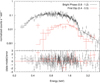 |
Fig. 8. Phase-resolved X-ray spectra of the SRGE0758. The black data points represent the bright phase spectrum and were extracted for the phase interval 0.8 − 1.2. The black line shows the model fit with a reduced chi-square value of 1.02 (χ = 171 for 168 d.o.f.). The spectrum of the first dip (shown with red data points) was obtained from the phase at 0.4 − 0.5. The fit revealed a reduced χ2 of 1.51 (χ = 30 for 20 d.o.f.). |
Many ROSAT-discovered polars show a soft, blackbody-like radiation component from the bottom of the accretion column and its surroundings. However, we could not find evidence of such a blackbody component in the spectrum.
We calculated the unabsorbed fluxes with the “cflux” task in XSPEC. After ideal spectral fitting, we calculated the bolometric X-ray flux with XSPEC using the best-fit spectral parameters and a dummy response that covered the broad energy range between 10−6 and 104 keV. The bolometric correction factor was 1.28. Errors were calculated with the "error" command in XSPEC (90% significance). All the fit results and uncertainties are listed in Table 2.
Spectral parameters from the bright phase interval (ϕ = 0.8 − 1.2): spectral fit parameters, their uncertainties, fit statistics, and model bolometric fluxes.
We then wanted to better constrain the spectral parameters as a function of the spin phase and, in particular, the change in the column density through the main absorption dip. We therefore generated phase-resolved spectra using ten phase bins of equal length. The photons per phase bin were grouped again with 20 counts per spectral bin. The temperature of the MEKAL model was fixed at the bright phase temperature so that only the column density and the model normalization were allowed to vary. In the bottom panel of Fig. 7, the phase-dependent behavior of the column density is shown. It was NH = 0.5 × 1021 cm−2 for most of the phase bins and for the mean spectrum. During the first dip, a marked increase by almost a factor of ten (although with a large error bar) was observed, which was even in excess of the galactic column density. This accretion-related high column density is very similar or comparable with other well-known polars, for example, HU Aqr during its high accretion state (factor of ten; Schwarz et al. 2009).
A rough estimate of the mass accretion rate limit can be derived via the X-ray luminosity. If one assumes that the WD in SRGE0758 is a typical one, its likely mass is 0.8 M⊙ (Pala et al. 2022). We estimated Rwd for this mass using the Nauenberg (1972) mass–radius relation. If one further assumes that the X-ray luminosity is a good proxy for the accretion luminosity, Lacc ≃ LX, one gets Ṁ = LXR0.8/M0.8G = 8.3(7) × 10−11 M⊙ yr−1 (only flux error considered here). The accretion rate was calculated for the distance of 2733 pc (Bailer-Jones et al. 2021b). These authors also give a rather large confidence interval between 1225 pc and 4147 pc. Taking the uncertainty of the distance into account, the likely accretion rate lies in the interval Ṁ ≈ 2 − 19 × 10−11 M⊙ yr−1.
3.3.3. eROSITA all-sky surveys
In Fig. 9, X-ray images for the first four eROSITA all-sky survey (eRASS) scans of SRGE0758 are shown. The new object was detected in the first three scans but not in the last (eRASS4). The mean count rates and observation times are listed in Table 3. Because of the high ecliptic latitude of the object, every survey scanned the position of SRGE0758 quite often every four hours, thus building a farther deep-survey exposure (Freyberg et al. 2020).
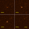 |
Fig. 9. Images of the CV during the four eROSITA all-sky surveys in the 0.2–2.3 keV range. During eRASS4, the object was in a low state. |
Observation log of the eROSITA all-sky surveys and pointed observations covering the location of SRGE0758.
We calculated the count rate upper limit at the position of the source in eRASS4 based on X-ray aperture photometry following the Bayesian approach described by Kraft et al. (1991). We collected observed counts, background counts, and exposure time within a circular aperture with a radius of rape = 30.5 arcsec at the 0.2 – 2.3 keV energy band. The aperture corresponds to a point spread function (PSF) encircled energy fraction of EEF = 0.75, which measures the fraction of total photons within the aperture. The X-ray flux decrease in eRASS1 and nondetection in eRASS4 suggest an overall X-ray emission cut in the object and indicate a different mass accretion state (see Fig. 10).
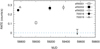 |
Fig. 10. Long-term X-ray light curve of SRGE0758 corresponding to eRASS1-4 and pointed eROSITA observations. Black arrow displays the upper flux limit of the eRASS4 survey for given sky position of the SRGE0758. |
3.4. Accretion geometry
The X-ray light curve of the object does not contain an eclipse of a WD. Therefore, we do not know the true orbital phase zero. The X-ray observations only revealed one bright hump with two consecutive dips. The optical variability obtained with TESS revealed the same photometric period, while the optical light curve shows just one hump. Under these circumstances, it is not possible to specify the location of the accretion column. But we can nevertheless derive a few constraints.
The increased absorption at the phase of the deep dip suggests an origin due to photo-electric absorption in the accretion stream. The second dip is likely caused by a self-eclipse of the accretion column by the WD itself. During the second dip, the accretion region is partially hidden behind the limb of the WD. Accordingly, this accretion region, which is visible for most of the orbital cycle, is located in the upper hemisphere (with respect to the orbital plane β < 90 ° , with β as the colatitude of the accretion region). The object does not show an eclipse; hence, the inclination is constrained to i < 75°.
The stream eclipse at the 0.4 phase can only occur if the orbital inclination is larger than the colatitude of the column (i > β). If our interpretation that the second dip is due to a self-eclipse is correct, then i + β ≃ 90°. The mid points of the two dips are separated by Δϕ ∼ 0.29 phase. Best visibility of the accretion region is then expected at half a cycle later, that is, about 0.2 phase units before the first dip. One would then expect to observe a clear maximum in the light curve due to the given best visibility of the accretion region, which is not clearly observed. Instead, there is an extended bright phase without a clear center or maximum.
The typical location of a stream dip in polars is between the 0.8 and 0.9 phases (e.g., Schwope et al. 2001). In polars with a pronounced bright-phase hump in the light curve, the dip is often located in the second half of the bright phase; that is, the dip occurs shortly after the bright phase center (i.e., approximately 0.1–0.2 phase units later). If our tentative geometry is correct, the situation in SRGE0758 is rather different, with the dip trailing the bright phase by 0.2 phase units. Such geometry seems to be unusual, but actually there are other polars that display similar photometric features, namely, QQ Vul (Belle et al. 2000) and V834 Cen (Schwope et al. 2008). The true orbital phase zero of these systems is known. In both objects, the true phase zero was located between the two consecutive dips.
4. Discussion and conclusion
We have analysed extended eROSITA and TESS observations of a serendipitously discovered X-ray source in the direction of the open cluster NGC 2516 that clearly does not belong to the cluster. The source is among the brightest X-ray objects among the eROSITA CalPV observations of the field, and it is an accretion-powered background object at a distance of about 1225–4147 pc. The cluster itself is at a distance of 400 pc (Terndrup et al. 2002). We also obtained SALT spectroscopic follow-up and time-resolved photometry from the South African Astronomical Observatory (SAAO). The eROSITA X-ray and optical TESS observations reveal a periodic variability of the source at 106 min. This is the only identified period in the system. The identification spectrum was obtained when the object was approximately 2 mag fainter compared to its Gaia measurements. The spectrum reveals hydrogen Balmer emission superposed on a flat or slightly blue continuum. All these features clearly identify the new object as a magnetic cataclysmic variable. It likely belongs to the AM Herculis or polar subclass, although an intermediate polar nature could not be ruled out completely. This identification is based on the occurrence of just one period in the system (the spin period of the WD) and the accretion rate changes, which is typically observed in polars. Also, the low state spectrum is similar to other polars.
The X-ray light curves were modulated by 100% on the 106 min period. The most pronounced structure in the light is an eclipse-like broad dip at phase 0.40, which we interpret as stream absorption. Stream eclipses are common among polars. They are observed in EF Eri (Beuermann et al. 1991), EK UMa (Clayton & Osborne 1994), QQ Vul (Beardmore et al. 1995), HU Aqr (Schwope et al. 2001), and UZ For (Warren et al. 1995), and they require that the magnetically guided accretion stream be lifted out of the orbital plane in order to cross the line of sight. The second dip is clearly revealed in the phase-folded X-ray light curve, but not so much in the individual cycles. It is tentatively identified as a possible self-eclipse of the emission region because no change of the HR or the column density was observed at this phase. The self-eclipse could be only grazing, as the X-ray flux stays finite at this phase. This interpretation is based on the observation that neither the HR nor the column density in the spectral fits show significant variability at this phase.
Due to the lack of a primary star eclipse or other information from spectral line variability, the true phase zero is unknown. But the fact that the 106-min photometric period is the same in both the TESS and eROSITA observations suggests a synchronous spin-orbital rotation, a typical property of polars (Warner 1995). A large portion of the polar population has orbital periods of less than two hours (Kuulkers et al. 2010), same as our new object. In addition, we did not encounter any change implying the WD spin, as seen in intermediate polars. In intermediate polars, accretion can occur in two ways: stream-fed or disk-fed. In either accretion scenario, the matter changes poles due to the WD spin, and this change itself breeds a beat period in periodograms from X-ray and optical light curves (Norton et al. 1997).
The mean optical light curve from TESS is not as complex as the X-ray light curve. The variation is very smooth and almost sinusoidal. The variability amplitude is likely small but cannot be properly quantified given the relative faintness of the star and the contamination due to a second object in the same pixel. The maxima of the TESS and eROSITA light curves are roughly coincident. We could not detect any sharp and strong accretion stream nor a curtain related absorption in the TESS light curves. The TESS minimum lies between the two dips in the X-rays but is closer to the first. Optical variability in polars may be caused by cyclotron beaming, geometric foreshortening of a heated accretion region, and obscuration of the light sources. Given the lack of detailed light curve information, we do not speculate on the origin of the TESS variability in SRGE0758.
The X-ray spectrum is compatible with single-temperature thermal plasma emission at around 10 keV, which is well in line with what is typically found in polars (Kuulkers et al. 2010). Additionally, polars have lower X-ray temperatures than intermediate polars (Mukai 2017). The new object lacks a soft blackbody component in its X-ray spectrum, which is often prominent in X-ray spectra of ROSAT-discovered polars Beuermann & Schwope (1994). This characteristic is similar to other polars discovered with XMM-Newton (Vogel et al. 2008; Ramsay et al. 2009; Webb et al. 2018), and the first eROSITA-discovered polar also seems to lack this component Schwope et al. (2022). The strength of the soft X-ray excess in polars has been a hotly debated topic (e.g., Vogel et al. 2008; Ramsay et al. 2009). It seems that the effective energy range of XMM-Newton, which cannot extend to extreme ultraviolet (EUV) wavelengths, makes it difficult to detect this component of reprocessed emission from the WD in some systems. Presumably, we are facing the same issue with eROSITA, which has a similar sensitivity range.
The optical identification spectrum has a flat continuum and contains broad hydrogen emission lines, which is a good indicator for magnetic accretors. The continuum neither reveals the WD nor the cyclotron harmonic emission nor the donor star. A detection of the donor cannot be expected given the large distance and the short orbital period, hence the late spectral type (Knigge et al. 2011, predict a spectral type later than M5.3) and thus faintness of the star. Another specific feature that needs to be discussed is the large-scale brightness change between the Gaia and SALT spectrum (∼1.8 mag). While orbital phase-dependent variability of up to four magnitudes may occur in polars, the brightness drop by about two magnitudes between the Gaia and SALT spectrum is more likely due to a reduced mass accretion rate. The lack of clearly detected helium lines is suggestive of a reduced accretion state. The nondetection in eRASS4, which occurred about five months prior to the SALT observations, supports this view. Accretion state transitions occur randomly in polars. The time they spend in these states also changes randomly and is thus unpredictable. The triggering mechanism is thought to be predominantly chromospheric activity in the donor star (Kafka & Honeycutt 2005). On the other hand, accretion state variations are not a unique indication of a polar. Also, intermediate polars are frequently being discovered in low states – the first perhaps being FO Aqr (e.g., Littlefield et al. 2020; Kennedy et al. 2020) followed by several others (e.g., Covington et al. 2022; Hill et al. 2022).
The position of the first dip with respect to the main X-ray hump in the light curve implies that the object has a very interesting accretion geometry. The column is not in the direction of the secondary star. The appearance of the stream dip after the main hump implies that the accretion spot is in a rather perpendicular position to the system. The accretion to the distant pole is more likely occur at high accretion states (Ferrario et al. 1989) in polars.
Previously, ROSAT and Swift observatories observed the NGC 2516, but SRGE0758 could not be detected by either mission. The object was probably in a low accretion state when these observations were conducted. The sensitivity of eROSITA together with its optimized scanning strategy led to the discovery of this object despite its large distance and its fluctuation between high and low states. It may be expected that the eROSITA will uncover many more magnetic CVs through systematic follow-up observations of all point-like X-ray sources found in the eRASS. In particular, there is a great chance of finding sources that evaded detection in the ROSAT all-sky survey by being in a low state at the time of observation, as the duty of polars might be as short as 50% (Hessman et al. 2000).
Acknowledgments
Samet Ok is supported by TUBITAK 2219-International Postdoctoral Research Fellowship Program for Turkish Citizens. Samet Ok acknowledges deep gratitude to the Leibniz Institute for Astrophysics Potsdam (AIP) and members of the X-ray astronomy group for the warm hospitality during his stay. This work was supported by the Deutsches Zentrum für Luft- und Raumfahrt (DLR) under grants 50 QR 2104, 50 OX 1901, and 50 OR 2203. Support by the Deutsche Forschungsgemeinschaft under grant Schw536/37-2 is gratefully acknowledged. This research has made use of data, software and/or web tools obtained from the High Energy Astrophysics Science Archive Research Center (HEASARC), a service of the Astrophysics Science Division at NASA/GSFC and of the Smithsonian Astrophysical Observatory’s High Energy Astrophysics Division. This paper includes data collected by the TESS mission. Funding for the TESS mission is provided by the NASA’s Science Mission Directorate. This work is based on data from eROSITA, the soft X-ray instrument aboard SRG, a joint Russian-German science mission supported by the Russian Space Agency (Roskosmos), in the interests of the Russian Academy of Sciences represented by its Space Research Institute (IKI), and the Deutsches Zentrum für Luft- und Raumfahrt (DLR). The SRG spacecraft was built by Lavochkin Association (NPOL) and its subcontractors, and is operated by NPOL with support from the Max Planck Institute for Extraterrestrial Physics (MPE). The development and construction of the eROSITA X-ray instrument was led by MPE, with contributions from the Dr. Karl Remeis Observatory Bamberg and ECAP (FAU Erlangen-Nuernberg), the University of Hamburg Observatory, the Leibniz Institute for Astrophysics Potsdam (AIP), and the Institute for Astronomy and Astrophysics of the University of Tübingen, with the support of DLR and the Max Planck Society. The Argelander Institute for Astronomy of the University of Bonn and the Ludwig Maximilians Universität Munich also participated in the science preparation for eROSITA. The eROSITA data shown here were processed using the eSASS software system developed by the German eROSITA consortium. We thank the anonymous referee for useful comments and suggestions which helped to improve the paper.
References
- Arnaud, K. A. 1996, ASP Conf. Ser., 101, 17 [Google Scholar]
- Bailer-Jones, C. A. L., Rybizki, J., Fouesneau, M., Demleitner, M., & Andrae, R. 2021a, AJ, 161, 147 [Google Scholar]
- Bailer-Jones, C. A. L., Rybizki, J., Fouesneau, M., Demleitner, M., & Andrae, R. 2021b, VizieR Online Data Catalog: I/352 [Google Scholar]
- Baluev, R. V. 2008, MNRAS, 385, 1279 [Google Scholar]
- Beardmore, A. P., Ramsay, G., Osborne, J. P., et al. 1995, MNRAS, 273, 742 [NASA ADS] [CrossRef] [Google Scholar]
- Belle, K. E., Howell, S. B., & Mills, A. 2000, PASP, 112, 343 [NASA ADS] [CrossRef] [Google Scholar]
- Beuermann, K., Thomas, H. C., & Pietsch, W. 1991, A&A, 246, L36 [NASA ADS] [Google Scholar]
- Beuermann, K., & Schwope, A. D. 1994, ASP Conf. Ser., 56, 119 [NASA ADS] [Google Scholar]
- Brunner, H., Liu, T., Lamer, G., et al. 2022, A&A, 661, A1 [NASA ADS] [CrossRef] [EDP Sciences] [Google Scholar]
- Buckley, D. A. H., Swart, G. P., & Meiring, J. G. 2006, SPIE Conf. Ser., 6267, 62670Z [Google Scholar]
- Buckley, D. A. H., Andreoni, I., Barway, S., et al. 2018, MNRAS, 474, L71 [NASA ADS] [CrossRef] [Google Scholar]
- Burgh, E. B., Nordsieck, K. H., Kobulnicky, H. A., et al. 2003, SPIE Conf. Ser., 4841, 1463 [NASA ADS] [Google Scholar]
- Clayton, K. L., & Osborne, J. P. 1994, MNRAS, 268, 229 [NASA ADS] [CrossRef] [Google Scholar]
- Covington, A. E., Shaw, A. W., Mukai, K., et al. 2022, ApJ, 928, 164 [NASA ADS] [CrossRef] [Google Scholar]
- Creevey, O. L., Sordo, R., Pailler, F., et al. 2023, A&A, in press, https://doi.org/10.1051/0004-6361/202243688 [Google Scholar]
- Dorman, B., & Arnaud, K. A. 2001, ASP Conf. Ser., 238, 415 [NASA ADS] [Google Scholar]
- Eyer, L., Audard, M., Holl, B., et al. 2023, A&A, in press, https://doi.org/10.1051/0004-6361/202244242 [Google Scholar]
- Feinstein, A. D., Montet, B. T., Foreman-Mackey, D., et al. 2019, PASP, 131, 094502 [Google Scholar]
- Ferrario, L., Wickramasinghe, D. T., & Tuohy, I. R. 1989, ApJ, 341, 327 [NASA ADS] [CrossRef] [Google Scholar]
- Fouesneau, M., Frémat, Y., Andrae, R., et al. 2023, A&A, in press, https://doi.org/10.1051/0004-6361/202243919 [Google Scholar]
- Frank, J., King, A. R., & Lasota, J. P. 1988, A&A, 193, 113 [NASA ADS] [Google Scholar]
- Freyberg, M., Perinati, E., Pacaud, F., et al. 2020, SPIE Conf. Ser., 11444, 114441O [Google Scholar]
- Gaia Collaboration (Brown, A. G. A., et al.) 2021, A&A, 649, A1 [NASA ADS] [CrossRef] [EDP Sciences] [Google Scholar]
- Hessman, F. V., Gänsicke, B. T., & Mattei, J. A. 2000, A&A, 361, 952 [NASA ADS] [Google Scholar]
- Hill, K. L., Littlefield, C., Garnavich, P., et al. 2022, AJ, 163, 246 [NASA ADS] [CrossRef] [Google Scholar]
- Kafka, S., & Honeycutt, R. K. 2005, AJ, 130, 742 [NASA ADS] [CrossRef] [Google Scholar]
- Kennedy, M. R., Garnavich, P. M., Littlefield, C., et al. 2020, MNRAS, 495, 4445 [NASA ADS] [CrossRef] [Google Scholar]
- Knigge, C. 2006, MNRAS, 373, 484 [NASA ADS] [CrossRef] [Google Scholar]
- Knigge, C., Baraffe, I., & Patterson, J. 2011, ApJS, 194, 28 [Google Scholar]
- Kraft, R. P., Burrows, D. N., & Nousek, J. A. 1991, ApJ, 374, 344 [Google Scholar]
- Kuulkers, E., Norton, A., Schwope, A., & Warner, B. 2010, Compact Stellar X-ray Sources, 421 [Google Scholar]
- Lamb, D. Q., & Masters, A. R. 1979, ApJ, 234, L117 [NASA ADS] [CrossRef] [Google Scholar]
- Liedahl, D. A., Osterheld, A. L., & Goldstein, W. H. 1995, ApJ, 438, L115 [CrossRef] [Google Scholar]
- Lightkurve Collaboration (Cardoso, J. V. D. M., et al.) 2018, Astrophysics Source Code Library [record ascl:1812.013] [Google Scholar]
- Littlefield, C., Garnavich, P., Kennedy, M. R., et al. 2020, ApJ, 896, 116 [NASA ADS] [CrossRef] [Google Scholar]
- Livio, M., & Pringle, J. E. 1994, ApJ, 427, 956 [NASA ADS] [CrossRef] [Google Scholar]
- Lomb, N. R. 1976, Ap&SS, 39, 447 [Google Scholar]
- Markley, F. L., & Crassidis, J. L. 2014, Fundamentals of Spacecraft Attitude Determination and Control (Springer) [CrossRef] [Google Scholar]
- Mewe, R., Gronenschild, E. H. B. M., & van den Oord, G. H. J. 1985, A&AS, 62, 197 [NASA ADS] [Google Scholar]
- Mukai, K. 2017, PASP, 129, 062001 [Google Scholar]
- Nauenberg, M. 1972, ApJ, 175, 417 [NASA ADS] [CrossRef] [Google Scholar]
- Norton, A. J., Hellier, C., Beardmore, A. P., et al. 1997, MNRAS, 289, 362 [NASA ADS] [Google Scholar]
- Oke, J. B. 1990, AJ, 99, 1621 [Google Scholar]
- Pala, A. F., Gänsicke, B. T., Belloni, D., et al. 2022, MNRAS, 510, 6110 [NASA ADS] [CrossRef] [Google Scholar]
- Predehl, P., Andritschke, R., Arefiev, V., et al. 2021, A&A, 647, A1 [EDP Sciences] [Google Scholar]
- Ramsay, G., & Cropper, M. 2004, MNRAS, 347, 497 [NASA ADS] [CrossRef] [Google Scholar]
- Ramsay, G., Rosen, S., Hakala, P., & Barclay, T. 2009, MNRAS, 395, 416 [NASA ADS] [CrossRef] [Google Scholar]
- Ricker, G. R., Winn, J. N., Vanderspek, R., et al. 2014, SPIE Conf. Ser., 9143, 914320 [Google Scholar]
- Ritter, H., & Kolb, U. 2003, A&A, 404, 301 [NASA ADS] [CrossRef] [EDP Sciences] [Google Scholar]
- Scargle, J. D. 1982, ApJ, 263, 835 [Google Scholar]
- Schwarz, R., Schwope, A. D., Vogel, J., et al. 2009, A&A, 496, 833 [NASA ADS] [CrossRef] [EDP Sciences] [Google Scholar]
- Schwope, A. D., Schwarz, R., Sirk, M., & Howell, S. B. 2001, A&A, 375, 419 [NASA ADS] [CrossRef] [EDP Sciences] [Google Scholar]
- Schwope, A. D., Brunner, H., Hambaryan, V., & Schwarz, R. 2002, ASP Conf. Ser., 261, 102 [NASA ADS] [Google Scholar]
- Schwope, A., Vogel, J., Schwarz, R., et al. 2008, The X-ray Universe 2008 (ESA), 73 [Google Scholar]
- Schwope, A. D., Worpel, H., Traulsen, I., & Sablowski, D. 2020, A&A, 642, A134 [NASA ADS] [CrossRef] [EDP Sciences] [Google Scholar]
- Schwope, A., Buckley, D. A. H., Malyali, A., et al. 2022, A&A, 661, A43 [NASA ADS] [CrossRef] [EDP Sciences] [Google Scholar]
- Sunyaev, R., Arefiev, V., Babyshkin, V., et al. 2021, A&A, 656, A132 [NASA ADS] [CrossRef] [EDP Sciences] [Google Scholar]
- Szkody, P. 1998, ASP Conf. Ser., 137, 18 [NASA ADS] [Google Scholar]
- Terndrup, D. M., Pinsonneault, M., Jeffries, R. D., et al. 2002, ApJ, 576, 950 [NASA ADS] [CrossRef] [Google Scholar]
- Tody, D. 1986, SPIE Conf. Ser., 627, 733 [Google Scholar]
- VanderPlas, J. T. 2018, ApJS, 236, 16 [Google Scholar]
- Vogel, J., Byckling, K., Schwope, A., et al. 2008, A&A, 485, 787 [NASA ADS] [CrossRef] [EDP Sciences] [Google Scholar]
- Wahba, G. 1965, SIAM Rev., 7, 409 [NASA ADS] [CrossRef] [Google Scholar]
- Warner, B. 1995, Cataclysmic Variable Stars (Cambridge University Press), 28 [CrossRef] [Google Scholar]
- Warren, J. K., Sirk, M. M., & Vallerga, J. V. 1995, ApJ, 445, 909 [NASA ADS] [CrossRef] [Google Scholar]
- Watson, M. G., King, A. R., Jones, M. H., & Motch, C. 1989, MNRAS, 237, 299 [NASA ADS] [CrossRef] [Google Scholar]
- Webb, N. A., Schwope, A., Zolotukhin, I., Lin, D., & Rosen, S. R. 2018, A&A, 615, A133 [NASA ADS] [CrossRef] [EDP Sciences] [Google Scholar]
- Wilms, J., Allen, A., & McCray, R. 2000, ApJ, 542, 914 [Google Scholar]
- Wu, K., & Kiss, L. L. 2008, A&A, 481, 433 [NASA ADS] [CrossRef] [EDP Sciences] [Google Scholar]
All Tables
Spectral parameters from the bright phase interval (ϕ = 0.8 − 1.2): spectral fit parameters, their uncertainties, fit statistics, and model bolometric fluxes.
Observation log of the eROSITA all-sky surveys and pointed observations covering the location of SRGE0758.
All Figures
|
Fig. 1. X-ray image of the NGC 2516 obtained by eROSITA. The white dashed circle marks the position of SRGE0758. False colors of the image were made using photon energies between 0.2 and 1.1 keV, 1.1 and 2.3 keV, and 2.3 and 5 keV for the red, green, and blue channels, respectively. The image displays an area of 1×1 deg. |
| In the text | |
|
Fig. 2. DSS image of the sky region around SRGE0758. The optical counterpart is marked with red lines. |
| In the text | |
|
Fig. 3. TESS light curve of SRGE0758 obtained for sector 35. Panel (a): background corrected TESS light curve in original time series. Panel (b): normalized light curve for sector 35. Panel (c): folded light curve of sector 35 according to Eq. (1) in normalized flux. |
| In the text | |
|
Fig. 4. Lomb-Scargle periodogram of the TESS and eROSITA observations. The main figure shows the over plotted power spectra of the object obtained from TESS and eROSITA, and the inset details the main peak of the TESS observations. The dashed black line shows a Gaussian line fit to the main peak. The red dashed line in the main frame gives the 99% significance level of the eROSITA power spectrum. The main period and its harmonics are indicated with the Ω symbol. The horizontal black dashed line within the inset indicates the 99% significance level for the TESS spectrum. |
| In the text | |
|
Fig. 5. SALT spectrum of the SRGE0758. The wavelength ranges strongly contaminated by sky lines or cosmic rays are indicated in gray. |
| In the text | |
|
Fig. 6. eROSITA 0.2 − 2.3 keV X-ray light curve of SRGE0758 with time bins of 100 s. The top row shows the data from ObsID 700018 and the lower row shows that of ObsID 700019. |
| In the text | |
|
Fig. 7. TESS, energy-resolved eROSITA light curves, HR and NH variations of SRGE0758 for ObsID 700019. Panel (a): TESS light curve obtained from sectors 31 and 37. Panels (b) and (c): X-ray data in the two indicated energy bands originally binned using 50 s time bins and averaged using a phase bin size of 0.005 phase units. Panel (d): HR obtained from 0.2 to 0.8 keV and 0.8 to 2.3 keV energy bands. Panel (e): column density variation. All light curves folded according to photometric period and T0, max in Eq. (1). |
| In the text | |
|
Fig. 8. Phase-resolved X-ray spectra of the SRGE0758. The black data points represent the bright phase spectrum and were extracted for the phase interval 0.8 − 1.2. The black line shows the model fit with a reduced chi-square value of 1.02 (χ = 171 for 168 d.o.f.). The spectrum of the first dip (shown with red data points) was obtained from the phase at 0.4 − 0.5. The fit revealed a reduced χ2 of 1.51 (χ = 30 for 20 d.o.f.). |
| In the text | |
|
Fig. 9. Images of the CV during the four eROSITA all-sky surveys in the 0.2–2.3 keV range. During eRASS4, the object was in a low state. |
| In the text | |
|
Fig. 10. Long-term X-ray light curve of SRGE0758 corresponding to eRASS1-4 and pointed eROSITA observations. Black arrow displays the upper flux limit of the eRASS4 survey for given sky position of the SRGE0758. |
| In the text | |
Current usage metrics show cumulative count of Article Views (full-text article views including HTML views, PDF and ePub downloads, according to the available data) and Abstracts Views on Vision4Press platform.
Data correspond to usage on the plateform after 2015. The current usage metrics is available 48-96 hours after online publication and is updated daily on week days.
Initial download of the metrics may take a while.