| Issue |
A&A
Volume 672, April 2023
|
|
|---|---|---|
| Article Number | A141 | |
| Number of page(s) | 14 | |
| Section | The Sun and the Heliosphere | |
| DOI | https://doi.org/10.1051/0004-6361/202245267 | |
| Published online | 12 April 2023 | |
Estimating the longitudinal magnetic field in the chromosphere of quiet-Sun magnetic concentrations⋆
1
Instituto de Astrofísica de Canarias, C/ Vía Láctea, s/n, 38205 La Laguna, Tenerife, Spain
e-mail: This email address is being protected from spambots. You need JavaScript enabled to view it.
2
Departamento de Astrofísica, Universidad de La Laguna, 38206 La Laguna, Tenerife, Spain
3
Institute for Solar Physics, Dept. of Astronomy, Stockholm University, AlbaNova University Centre, 10691 Stockholm, Sweden
4
Consejo Superior de Investigaciones Científicas, Spain
Received:
22
October
2022
Accepted:
22
January
2023
Abstract
Context. Details of the magnetic field in the quiet-Sun chromosphere are key to our understanding of essential aspects of the solar atmosphere. However, the strength and orientation of this magnetic field have not been thoroughly studied at high spatial resolution.
Aims. We aim to determine the longitudinal magnetic field component (B∥) of quiet-Sun regions depending on their size.
Methods. We estimated B∥ by applying the weak-field approximation to high-spatial-resolution Ca II 854.2 nm data taken with the Swedish 1 m Solar Telescope. Specifically, we analyzed the estimates inferred for different spectral ranges using the data at the original cadence and temporally integrated signals.
Results. The longitudinal magnetic field in each considered plasma structure correlates with its size. Using a spectral range restricted to the line core leads to chromospheric longitudinal fields varying from ∼50 G at the edges to 150–500 G at the center of the structure. These values increase as the spectral range widens due to the photospheric contribution. However, the difference between this contribution and the chromospheric one is not uniform for all structures. Small and medium-sized concentrations show a steeper height gradient in B∥ compared to their chromospheric values, so estimates for wider ranges are less trustworthy. Signal addition does not alleviate this situation as the height gradients in B∥ are consistent with time. Finally, despite the amplified noise levels that deconvolving processes may cause, data restored with the destretching technique show similar results, though are affected by smearing.
Conclusions. We obtained B∥ estimates similar to those previously found, except for large concentrations and wide spectral ranges. In addition, we report a correlation between the height variation of B∥ compared to the chromospheric estimates and the concentration size. This correlation affects the difference between the photospheric and chromospheric magnetic flux values and the reliability of the estimates for wider spectral ranges.
Key words: Sun: chromosphere / Sun: photosphere / methods: data analysis / methods: observational / Sun: magnetic fields
Movies associated to Figs. 3, 7, and 10 are only available at https://www.aanda.org
© The Authors 2023
 Open Access article, published by EDP Sciences, under the terms of the Creative Commons Attribution License (https://creativecommons.org/licenses/by/4.0), which permits unrestricted use, distribution, and reproduction in any medium, provided the original work is properly cited.
This article is published in open access under the Subscribe to Open model. This email address is being protected from spambots. You need JavaScript enabled to view it. to support open access publication.
1. Introduction
Magnetic fields play a crucial role in explaining diverse processes throughout the solar atmosphere. However, the physical conditions in the chromosphere hinder the study of magnetic fields in this layer, which is key for linking the photospheric and coronal field topologies.
Polarization measurements in the photosphere of the quiet Sun show magnetic elements of diverse sizes and lifetimes. These structures are divided into a network (Sheeley 1967) and an internetwork (Livingston & Harvey 1975; Smithson 1975). The former consists of nearly vertical magnetic flux tubes expanding with height due to force imbalances. Network structures are bright due to their lower opacity (Spruit 1976) and harbor kG magnetic fields. In contrast, the internetwork is formed by small and short-lived structures randomly wandering due to convective motions until they merge with the network (e.g., Zirin 1985; Centeno et al. 2007; Martínez González & Bellot Rubio 2009; Gošić et al. 2014). These structures often appear as bipolar features linked by magnetic loops (e.g., Centeno et al. 2007; Martínez González & Bellot Rubio 2009). Internetwork fields have strengths of the order of hG (e.g., Khomenko et al. 2003; Asensio Ramos et al. 2007; Martínez González et al. 2007; Danilovic et al. 2016) and are crucial to our understanding of the quiet-Sun magnetism.
The coupling of the quiet-Sun magnetic field between the photosphere and the outer atmosphere is often described by umbrella-shaped canopies rising from network structures and expanding higher up. However, the inference of hG fields in the internetwork led to more complex schemes, such as the multiscale carpet model (Schrijver & Title 2003) where low-lying canopies link network and internetwork. In addition, the omnipresence of the internetwork suggests that it may contain an important fraction of the photospheric magnetic flux, thereby contributing greatly to the energy balance of the solar atmosphere (Trujillo Bueno et al. 2004). In this regard, Gošić et al. (2014) found internetwork magnetic flux values resembling those in the network and active regions and highlighted the importance of the internetwork as a contributor to the network flux. Moreover, internetwork fields are able to travel higher up across the photosphere (e.g., Martínez González et al. 2010; Gömöry et al. 2013).
Despite great efforts made over the years, the magnetism of the quiet-Sun photosphere is not totally understood due to the small scale and weakness of the signals of the observed magnetic elements (see the reviews by Trujillo Bueno et al. 2006, Sánchez Almeida & Martínez González 2011, and Bellot Rubio & Orozco Suárez 2019). These drawbacks are exacerbated in the chromosphere, where the particle density drops. This decrease benefits the expansion of magnetic fields leading to weak polarization signals. For instance, Stokes V amplitudes in the Ca II 854.2 nm line in the quiet Sun are of about 10−2–10−3 relative to the continuum intensity. However, noise levels below 10−3.5 are required to detect linear polarization induced by the Zeeman effect in the λ8542 line (de la Cruz Rodríguez et al. 2012). For field strengths of between 10 and 100 G, the Hanle effect also contributes to the linear polarization of this line. In this last case, the expected Stokes Q and U signals at disk center are of the order of 10−4 (Manso Sainz & Trujillo Bueno 2010). In addition, a low collisional rate causes a weak coupling of the radiation to the local physical conditions, which invalidates the assumption of local thermodynamic equilibrium (LTE).
Fortunately, the use of circular polarization measurements in Ca II 854.2 nm has shed light on the magnetism of the quiet-Sun chromosphere. For example, the analysis of these measurements, combined with information in other spectral lines, has allowed the study of the interaction of rising small-scale internetwork loops with network loops and the role of cancellations of opposite-polarity internetwork photospheric fields in the local chromospheric heating (Gošić et al. 2018, 2021).
In fact, the chromospheric heating is another key aspect related to the magnetic field in the quiet-Sun chromosphere. Diverse mechanisms can heat the chromosphere (e.g., Kalkofen 1989; Khomenko & Collados 2012; Priest et al. 2018), but it is the Ohmic current dissipation that greatly contributes in the low-mid chromosphere of bright points and plages (Morosin et al. 2022). This predominance in the chromospheric heating makes the inference of the chromospheric magnetic field in quiet-Sun magnetic elements an appealing task as part of further exploration.
Despite the availability of diverse nonLTE inversion codes, the weak-field approximation (WFA) is commonly used to estimate the chromospheric magnetic field because it requires little time and is relatively straightforward (see Sect. 3.1). Specifically, this technique works well for measurements in the λ8542 line (Jennerholm Hammar 2014; Centeno 2018). According to Centeno (2018), the longitudinal field estimates are reliable for field strengths up to 1.2 kG, but are underestimated for noise levels of 10−3 in units of the continuum intensity.
Given its importance, we aim to characterize the magnetic field of quiet-Sun structures depending on their size using high-spatial-resolution data taken in the Ca II 854.2 nm line with the Swedish 1m Solar Telescope (SST; Scharmer et al. 2003). In this study, we determined the longitudinal magnetic field by applying the WFA to different spectral ranges across the line. In addition, we analyzed the estimates obtained from data at the original cadence and temporally integrated signals that mimic longer scanning times.
2. Observation and data reduction
On August 1, 2019, we acquired four time series of quiet-Sun regions at different positions over the center of the solar disk with the CRisp Imaging SpectroPolarimeter (CRISP, Scharmer 2006; Scharmer et al. 2008) attached to the SST. Table 1 shows some observing characteristics of each sequence. Seeing conditions were good during the observing run except in the late morning. We therefore only analyzed the first 35 scans of the last time series.
Heliocentric coordinates of the FOV center at the beginning of the observing run, time interval, and number of scans of each dataset.
Each time series consists of full-Stokes measurements in the Ca II 854.2 nm line at high spatial resolution. The line was sampled at 21 nonequidistant wavelength positions between ±1.040 Å from the line center using steps of 65 mÅ in the core and wider in the wings, plus two extra points at ±1.755 Å. We acquired 12 accumulations per wavelength position. As the exposure time of each accumulation is 17 ms (with four modulation states), each sampling was completed every 31.5 s. The field of view (FOV) is ∼55″×55″ and the pixel size 0.057″.
We performed the data reduction using the SSTRED pipeline (de la Cruz Rodríguez et al. 2015; Löfdahl et al. 2021). Images were restored with the Multi-Object-Multi-Frame-Blind-Deconvolution technique (MOMFBD, Löfdahl & Scharmer 1994; van Noort et al. 2005). Finally, we performed the polarimetric calibration on a pixel-by-pixel basis as proposed by van Noort & Rouppe van der Voort (2008). The noise level in the resulting Stokes Q, U, and V images is 2.3–2.8×10⁻³, 2.4–2.6×10⁻³, and 2.2–2.5×10⁻³ as measured on the Q/I0, QS, U/I0, QS, and V/I0, QS maps at the first observed wavelength of each series. I0, QS refers to the first observed wavelength intensity averaged over a very quiet area. Given the weak linear polarization signals expected in the quiet-Sun chromosphere (see Sect. 1), the polarimetric sensitivity of our spectropolarimetric data is not large enough to detect them in all the studied elements.
3. Analysis
Considering their brightness and conspicuous Stokes V signals, we search for field concentrations in the Ca II 854.2 nm intensity filtergrams at −1.755 Å and magnetograms at ±0.39 Å with the CRISPEX tool (Vissers & Rouppe van der Voort 2012). We found 31 concentrations of different sizes, which we delimited by adopting thresholds of intensity at −1.755 Å and circular polarization at −0.39 Å of 0.95I0, QS and ±4×10⁻³I0, QS. The red rectangles overplotted in Fig. 1 display the locations of these structures. Most of the concentrations are visible during the entire run and often undergo fragmentations and mergings with other nearby concentrations. Such interactions are also included in this study.
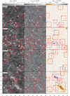 |
Fig. 1. Intensity filtergrams of the Ca II 854.2 nm line core and at −1.755 Å (left and middle columns), and blue-wing magnetograms of Ca II 854.2 nm at −0.39 Å from the line center (right column). The red rectangles show the positions of the analyzed structures. The time stamp of each scan in UT is shown in the upper-left corner labels. Axes are labeled in arcseconds. |
While static plane-parallel mediums show antisymmetric Stokes V profiles, asymmetries appear in realistic model atmospheres. These asymmetries are mainly due to velocity gradients along the line of sight (LOS) and can be enhanced by magnetic-field gradients with height (Illing et al. 1975; Auer & Heasley 1978). Additionally, the presence of different Ca II isotopes in the solar atmosphere also induces asymmetries in the λ8542 line (Leenaarts et al. 2014). We used an automated code to identify pixels with two-lobed V profiles. Before that, we corrected the circular polarization signals for residual crosstalk from Stokes I similarly to Ortiz et al. (2014), resulting in noise levels of 2.1–2.4×10⁻³ as measured on the V/I0, QS maps at the first observed wavelength of each sequence. We also applied a principal component analysis denoising technique (PCA, Pearson 1901; Hotelling 1933) to the original circular polarization signals, leading to better-defined V profiles that prevent detection errors. Specifically, we used four eigenvectors for the Stokes V profiles in the first and third series and five in the second and fourth ones. We also smoothed the V profiles with a boxcar average of a width of 2 pixels to ease the detection of the desired pixels. Finally, the subsequent analysis was performed using the signals resulting from the application of the PCA technique.
In addition to using the data at the original cadence, we analyzed the results from different scanning times (Δt) to inspect the variation of the longitudinal magnetic field (see Sect. 3.1) with the signal addition, in the hope of increasing the detectability of weaker fields. For this aim, we first identified the scans showing each structure and grouped them as sets of two, four, and ten scans. Then, we combined the two-lobed Stokes V signals and the corresponding Stokes I profiles at each pixel according to each set of scans to imitate observations with Δt of 1.05, 2.10, and 5.25 minutes. We also performed these combinations using all scans displaying each structure. We ruled out pixels with complex V profiles by considering that their signals are zero. To avoid signal cancellation, we also discarded pixels with reversed polarities compared to that prevailing in each structure.
3.1. Application of the WFA
The WFA can be applied when the Zeeman splitting is much smaller than the Doppler width of the spectral line under consideration and the longitudinal component of the magnetic field is constant along the LOS (see Sect. 9.6 in Landi Degl’Innocenti & Landolfi 2004). Under these circumstances, the observed Stokes V profile is related to the observed Stokes I profile as
 (1)
(1)
with  , where λ0 and geff are the central wavelength (in Å) and the effective Landé factor of the line, respectively. The angle γ is the inclination of the magnetic field with respect to the LOS direction. The longitudinal component of the magnetic field vector is B∥ = B cos γ, with B the field strength (in G). The observed profile I(λ) is assumed to be the intensity that would emerge with zero magnetic field. The filling factor f is the fractional area occupied by the magnetic component within the resolution element. For simplicity, we assume f = 1. Thus, the shape of Stokes V is proportional to the derivative of Stokes I scaled by the B∥ estimate.
We compute B∥ as the maximum-likelihood estimation from Eq. (1) assuming Gaussian noise with zero mean and variance σ2, which leads to
 (2)
(2)
3.2. Definition of the analyzed spectral ranges
The Ca II 854.2 nm line covers a large range of formation heights (e.g., Uitenbroek 2006; Cauzzi et al. 2008; Quintero Noda et al. 2016). Its core is formed in the low- to mid-chromosphere, while its wings have a photospheric contribution. The variation from the LTE wings to the nonLTE chromospheric core occurs at ±0.03–0.04 nm from the line center (Cauzzi et al. 2008). Therefore, the estimation of B∥ values from the low- to mid-chromosphere is possible if the spectral range is restricted to the line core (Carlin & Asensio Ramos 2015). Given its wide formation region, delimiting spectral ranges in the λ8542 line is a common method to infer B∥ at certain heights (e.g., de la Cruz Rodríguez et al. 2013; Esteban Pozuelo et al. 2019; Morosin et al. 2020). Recently, this approach was also applied to synthetic data in the Mg II h and k lines (Afonso Delgado et al. 2023). In this paper, we applied Eq. (2) to different spectral ranges across the line to inspect how the B∥ estimates differ. Specifically, we selected almost all the spectral sampling (Δλ = ±1.040 Å), a limited range including both lobes of the V profile (±0.325 Å), and the inner-core positions (±0.130 Å). Hereafter, we denote these ranges as Δλ1, Δλ2, and Δλ3, respectively.
4. Results
The analyzed quiet-Sun structures evolve differently with time. While some of them undergo fragmentations, others either grow as they merge with nearby chunks or expand before decreasing. All cases show two-lobed V profiles coinciding with Stokes I signals that sometimes show asymmetries.
We divided the structures we found into three groups: small, medium-sized, and large field concentrations based on their aspect and size at the original cadence. Small field concentrations are elements with lengths of 0.45″–1.2″ wandering around granules. Medium-sized ones seem to be chains of magnetic elements expanding 3.5″–5.5″ between granules. Finally, large concentrations are fixed structures spreading over 10″–20″.
Figure 2 shows histograms of the number of pixels with two-lobed V profiles and B∥ estimates for each Δλ per group, which are normalized to the number of scans and pixels throughout the time sequences in each group (∼96×103, 266×103, and 682×103 pixels for small, medium-sized, and large concentrations), respectively. On average, pixels inside small, medium-sized, and large concentrations represent 0.06%, 0.13%, and 2.39% of the FOV per frame, respectively.
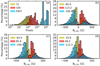 |
Fig. 2. Histograms of the number of pixels with two-lobed Stokes V signals (panel a), and B∥ values for Δλ1, Δλ2, and Δλ3 (panels b–d) in the studied cases. Distributions of pixels within small, medium-sized, and large field concentrations are colored in yellow, red, and blue, respectively. The median value of each distribution is shown in the upper-left corner of the panels. |
The distribution of the number of pixels with two-lobed V signals in large concentrations diverges from those in small and medium-sized ones. The former has two compact peaks standing for the two cases classified as large concentrations, while the latter two groups show broader size variability. Small concentrations tend to show negative polarity and often have B∥ values below 250 G for all Δλ. Medium-sized concentrations usually have positive polarity and harbor estimates below 400 G. The distributions of the large concentrations are smoother and reach B∥ values above 400 G. In addition, most of the pixels in large concentrations have negative polarity, which is the polarity of the largest structure. Generally, all distributions appear shifted to weaker estimates as Δλ narrows down.
All cases of each group share similar properties. We therefore describe them by showing one case for each group.
4.1. Small field concentrations
We identified 19 cases as small concentrations. They appear in intergranular lanes and are highly influenced by neighboring granules. We focus on the case labeled ‘3’ in the first row of Fig. 1. During its temporal evolution (see the movie attached to Fig. 3), small positive-polarity field concentrations appear between granules and move closer to each other until they form a single structure. After that, the structure changes its shape in reaction to the motion of the surrounding granules.
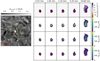 |
Fig. 3. Magnetograms at −0.39 Å and B∥ estimates on a small field concentration at different Δt. Left: Ca II 854.2 nm intensity filtergram at −1.755 Å. The yellow rectangle encloses the region shown on the right-hand side. Right (from top to bottom): blue-wing magnetograms at −0.39 Å and B∥ estimates from Δλ1, Δλ2, and Δλ3. Pink contours delimit the structure, black ones enclose pixels with two-lobed V signals inside it. The plus symbols (+) and crosses (×) mark the pixels shown in the two upper and lower rows of Fig. 4, respectively. Major tick marks represent 1″. A movie showing the temporal evolution of the parameters displayed in this figure is available online. |
Figure 3 also displays the variation of the blue-wing magnetogram (at −0.39 Å) and B∥ with the scanning time Δt. At the original cadence, estimates usually range from 100 to 360 G for Δλ1, and decay to 80–250 G and to 40–150 G for Δλ2 and Δλ3. Due to its dynamic behavior, the structure appears larger in maps at long Δt. Furthermore, V signals and B∥ estimates vary with Δt depending on the individual I and V profiles that are summed and the number of scans involved. Despite pixel-by-pixel differences, the estimates obtained for each Δλ do not differ significantly with Δt. We remind the reader that Δt refers to the time used to calculate the averaged Stokes I and V profiles (see Sect. 3).
We assessed the validity of the WFA conditions by comparing the observed Stokes V profiles to the I derivatives scaled by the estimates for each Δλ. Figure 4 displays these comparisons at two different locations as Δt increases. The two upper and lower rows show the I and V profiles from a pixel at the center and from another closer to the edge of the concentration, respectively. The plus symbols (+) and crosses (×) in Fig. 3 indicate these two specific locations. Although these locations do not share the same features, their I and V signals rely on the imprints left at these pixels during the instants involved in the signal addition. Consequently, all the estimates vary with the scanning time. We note that the gradient between the estimates obtained for each Δλ changes very little with Δt.
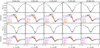 |
Fig. 4. Stokes I and V profiles emerging from a small concentration for different Δt (black dots). For visualization purposes, intensity profiles are normalized by the percentage of scans involved in the signal addition. Violet, orange, and red curves stand for the δI(λ)/δλ functions scaled by −CB∥ for Δλ1, Δλ2, and Δλ3, respectively. B∥ values for Δλ1, Δλ2, and Δλ3 in G are shown on each panel in violet, orange, and red. |
From a qualitative comparison, we observe a systematic divergence between the Stokes V profiles and the scaled I derivatives at the position of the blue lobe. Both curves only match in some pixels for Δλ3 (as in the fourth row of Fig. 4), but they slightly differ in others due to a relative shift between Stokes I and V at the line core (see the second row). This relative shift may be due to the coexistence of multiple components in the same resolution element. Using wider spectral ranges, the divergences between the V profiles and the scaled I derivatives remain regardless of Δt.
At this point, we note that we only describe the goodness of the fits from a qualitative point of view. A quantitative description is also possible. In that case, we would conclude that the quality worsens with Δt because the noise level for V/I decreases with the square root of the number of scans involved in each sum. This is mostly a consequence of the WFA not being able to explain the observations independently of Δt. As such a conclusion seems counterintuitive to what we observe from a naked-eye comparison, we opted for a qualitative description of the quality of the fits.
In addition, we observe that the fit quality between Stokes V and the scaled I derivatives at the outer-wing positions improves close to the concentration edge (fourth row in Fig. 4). To examine this further, we compared the synthetic Ca II 854.2 nm V profiles resulting from two model atmospheres with the STiC code (de la Cruz Rodríguez et al. 2019). The model atmospheres are based on the FALC model (Fontenla et al. 1993) to which we added B∥ values monotonically decreasing between log(τ500) = 1.3 and −5.3: (1) from 1000 to 100 G, and (2) from 300 to 100 G. We observe similarities in the outer-wing positions of the synthetic V profiles (shown in Fig. 5) and the observed ones, which indicates the high sensitivity of the V signals of the outer-wings to B∥ in the photosphere. Therefore, the fit quality in the outer-wing positions relies not only on the spectral range but also on the pixel location, as the field concentrations fan out with height. Other features may involve gradients in other parameters or the presence of an unresolved magnetic component not included here for simplicity.
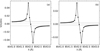 |
Fig. 5. Synthetic V profiles computed from different gradients in B∥ between log(τ500) = 1.3 and −5.3: from 1000 to 100 G (panel a) and from 300 to 100 G (panel b). The dashed gray lines mark the V values at the first and last wavelength positions, and the dotted gray lines indicate zero polarization signal. |
In view of the above findings, we compared the estimates for Δλ3 and the outer-wing positions (between ±1.040 and ±0.520 Å), from which we expect mainly chromospheric and photospheric contributions, respectively. We denote the latter range as Δλ4. As it may change with height, we delimited the structure again using intensity maps at −0.520 Å, where we still discern the structure despite the presence of fibrils. However, Figs. 6a,b show that the structure barely varies with height, whereas B∥ varies conspicuously. Central and outer regions of the concentration show significant height gradients in B∥ that resemble those used in the synthesis with STiC. Moreover, these gradients are consistent with time and are independent of the profile smoothing and of the noise decrease, as they appear regardless of Δt (see Fig. 4). Therefore, WFA conditions cannot be satisfied by adding signal.
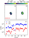 |
Fig. 6. Chromospheric and photospheric estimates in the small concentration at the original cadence (panels a and b), and temporal evolution of the corresponding magnetic flux (panel c). Major tick marks represent 1″. Black contours enclose pixels with two-lobed V profiles. We note that the values represented in panels a and b are saturated using different scales, which range from 0 to 175 G and from 100 to 1000 G, respectively. |
Finally, we computed the magnetic flux from the chromospheric and photospheric contributions using the expression
 (3)
(3)
where B∥(i, j) is the estimate for Δλ3 and Δλ4 at a pixel with coordinates (i, j), and ΔA is the pixel area. Specifically, the B∥ values used in Eq. (3) are those estimated at the original cadence. Figure 6c shows the resulting magnetic flux values, which vary with time depending on the temporal evolution of the structure. In addition, given the height gradient in B∥, the photospheric and chromospheric magnetic flux values differ by one order of magnitude during the time interval showing this case (see also Table 2).
Statistics on the chromospheric and photospheric magnetic flux in the depicted field concentrations.
4.2. Medium-sized field concentrations
We classified ten cases as medium-sized field concentrations; they have a practically fixed position and are observed as stable structures. In this subsection, we show an analysis of the case labeled ‘3’ in the second series (see Fig. 1), which is portrayed in Fig. 7. This positive-polarity case undergoes fragmentations and mergings (see the animation attached to Fig. 7). At the original cadence, the B∥ estimates for Δλ1 and Δλ2 are usually above 200 G and exceed 350 G at the center of the structure. These values are weaker for Δλ3 overall, reaching ∼250–300 G. Because of its stable behavior, B∥ maps barely change for Δt < 5.25 min.
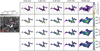 |
Fig. 7. Magnetograms at −0.39 Å and B∥ maps on a medium-sized concentration for different Δt. The plus symbols (+) and crosses (×) mark the pixels displayed in the two upper and lower rows of Fig. 8, respectively. Same layout as in Fig. 3. An animated version of this figure displaying the temporal evolution of this case is available online. |
The intensity profiles at the center of the concentration are different from those emerging closer to the edges, as shown in the upper and lower rows of Fig. 8. Locations close to the edge usually show line asymmetries and shifts, which may indicate that the physical conditions at the center of the structure are firmer than in the outer regions. In particular, the intensity profiles represented in the lower panels display slight asymmetries compared to those in the upper rows. Stokes V profiles also differ as amplitudes weaken away from the center. Aside from the V amplitude variations, we do not find changes with Δt worth mentioning. Regarding the B∥ estimates, the central and outer locations of the concentration show values of ∼420 and 260 G for Δλ1 at the original cadence, respectively. These B∥ values weaken by about 60 G and 100–200 G for Δλ2 and Δλ3, respectively. Moreover, the gradient between the estimates for each spectral range is stable with Δt and comparable to the individual values.
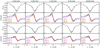 |
Fig. 8. Stokes I and V profiles coming from the depicted medium-sized concentration for different Δt, and their comparison to the Stokes I derivatives scaled by −CB∥ for Δλ1, Δλ2, and Δλ3, respectively. Same layout as in Fig. 4. |
We also compared the mostly chromospheric and photospheric B∥ estimates in this structure. The inferred values diverge significantly (see Figs. 9a,b), having median values of 105 and 524 G, respectively. Thus, the magnetic flux values for Δλ3 and Δλ4 differ again by one order of magnitude (Fig. 9c and Table 2) but, unlike the small case, they are stable with time. The height gradient in B∥ also explains the poor fit quality between the V profiles and the scaled I derivatives for Δλ1 and Δλ2. In contrast, fits are usually better for Δλ3, although they are affected by relative shifts between Stokes I and V at some positions. All in all, the estimates for wider spectral ranges are unsafe as the WFA conditions are unfulfilled.
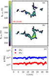 |
Fig. 9. Chromospheric and photospheric B∥ estimates in the medium-sized case at the original cadence (panels a and b), and temporal evolution of the corresponding magnetic flux (panel c). Major tick marks represent 1″. Black contours enclose pixels with two-lobed V profiles. We note that the values represented in panels a and b are saturated using different scales, which range from 0 to 400 G and from 100 to 1200 G, respectively. |
4.3. Large field concentrations
We identified two cases of large field concentrations; they are labeled ‘1’ and ‘2’ in the last row of Fig. 1 and may be an example of enhanced network. We focus on case 2, shown in Fig. 10, the polarity of which is negative.
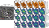 |
Fig. 10. Magnetograms at −0.39 Å and B∥ estimates on a large concentration for different Δt. The plus symbols (+) and crosses (×) mark the pixels shown in the two upper and lower rows of Fig. 11, respectively. The yellow rectangle delimits the region displayed on the right-hand side. Same layout as in Fig. 3. A movie showing the temporal evolution of the parameters displayed in this figure is available online. |
The movie attached to Fig. 10 shows that the B∥ values seem to oscillate with time, mostly at the center of the structure. As these oscillations coincide with overall intensity fluctuations, we think they are related to seeing instabilities instead of actual changes in the structure. At the original cadence, we infer estimates that progressively increase from the edges to the center of the structure, where they are of about −750 G for Δλ1. The B∥ maps for Δλ2 and Δλ3 are similar to that obtained for Δλ1, though estimates are weaker reaching up to −650 and −550 G, respectively. In addition, the concentration grows with Δt due to interactions with nearby structures and to the variable seeing conditions, whereas B∥ values weaken globally.
At the original cadence, asymmetries and blueshifts are apparent in the intensity profiles from the center of this concentration and from a pixel closer to the edge (see upper and lower rows of Fig. 11, respectively). These features persist with the scanning time until they soften at the longest Δt due to the profile smoothing. At the same time, V amplitudes decrease with the distance to the center of the structure and barely change with Δt. As a result of these changes along the concentration, B∥ values differ significantly depending on the pixel location. We find that, at the original cadence, estimates range from −500 to −700 G and from −180 to −260 G for the different Δλ at the center and closer to the edge, respectively. These B∥ gradients are stable with Δt, and so the conditions along the formation region related to the used spectral ranges hardly vary with time.
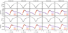 |
Fig. 11. Stokes I and V profiles coming from the depicted large concentration at different Δt, and their comparison to the Stokes I derivatives scaled by −CB∥ for Δλ1, Δλ2, and Δλ3, respectively. Same layout as in Fig. 4. |
Although not displayed, the difference between the mostly chromospheric and photospheric estimates in this concentration is not as significant as in smaller structures. The median values in this case for Δλ3 and Δλ4 are −160.7 and −360.3 G, respectively. Consequently, the photospheric magnetic flux is three to four times greater than the chromospheric flux (see Table 2). Similarly to the medium-sized case, the magnetic flux values inferred in this concentration have a stable temporal evolution. The reduced difference between the photospheric and chromospheric estimates may explain a better match between Stokes V and the scaled I derivatives regardless of the spectral range, scanning time, and location.
5. Discussion
Assuming WFA conditions, the reliability of the estimates for wide spectral ranges seems to rely on the concentration size. Small and medium-sized field concentrations have steeper time-independent height gradients in B∥ compared to their chromospheric B∥ values than the large ones, which leads to unreliable estimates of the former as the WFA requisites are unfulfilled. On the contrary, estimates for inner-core ranges are usually reliable in all concentrations.
Despite its assets, some observers may employ other restoration methods on the basis of the liabilities of MOMFBD. In this section, we compare results from data restored with different methods in order to decipher whether or not the restoration technique is related to the fulfillment of WFA conditions. In addition, as the WFA is widely used, we also discuss our results by comparing them to previous studies that used similar data.
5.1. Results from differently restored data
MOMFBD is a successful image-correction technique. However, its application comes with high computational cost and may lead to amplified noise levels (Puschmann & Beck 2011).
Alternatively, images can be restored by adding the accumulations acquired per wavelength position. In this case, most of the reduction process is carried out using the CRISPRED pipeline (de la Cruz Rodríguez et al. 2015) and the effects of seeing in observations are partially corrected by applying the destretching technique. During this process, differential motions in small subfields of the wide-band images, which are previously derotated and aligned, are measured using cross-correlation. After combining accumulations, the polarimetric calibration is performed as in van Noort & Rouppe van der Voort (2008). Finally, each pair of images with orthogonal polarization states, recorded simultaneously by the narrow-band cameras, are combined to remove the seeing-induced polarization, and the residual crosstalk is corrected. We also corrected each monochromatic polarization image for high-frequency polarimetric interference fringes in a similar way to Pietrow et al. (2020). As each image is apodized in this process, we clipped the blurred edges of the output polarization maps, obtaining smaller images. The noise level of the resulting Stokes V images is in the range of 1.8–2.5×10⁻³ measured on the V/I0 maps at the first observed wavelength for each series. We refer to the datasets restored with and without the MOMFBD technique as M and NM datasets, respectively.
We examined 27 of the cases shown in Fig. 1 because some of them are partially or completely beyond the image boundaries of the NM datasets. Each case has been delimited using thresholds of intensity at −1.755 Å and V(λ)/I(λ) at −0.39 Å of 0.95I0, QS and 4×10⁻³, respectively. After that, we estimated B∥ by applying the WFA in pixels with two-lobed V profiles and analyzed their variation with the scanning time, Δt (see Sect. 3).
Figure 12 shows the B∥ estimates obtained for the cases depicted in Sect. 3 using the NM datasets. The physical quantities in this figure appear smeared in comparison to those in Figs. 3, 7, and 10. We observe not only blurrier intensity images but also smoother B∥ estimates. Indeed, the latter are generally 50–100 G weaker for all Δt. These differences between both datasets appear because the intensity signal in each pixel is spread out over its surroundings in the NM datasets, as neither the blurring effect of the telescope point spread function (PSF) nor the low-altitude seeing is corrected. Nonetheless, the smearing relies on the concentration size. This correlation is clear in Fig. 13, where the divergence of the I and V profiles from the NM and M datasets increases as the concentration size decreases.
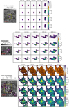 |
Fig. 12. Details of the cases shown in Figs. 3, 7, and 10 using the NM datasets. Left: Ca II 854.2 nm intensity filtergrams at −1.755 Å. The yellow rectangles superimposed over the small and large concentrations enclose the regions shown zoomed-in on the right-hand side. Right: magnetograms at −0.39 Å and B∥ estimates for each Δλ and Δt. The plus symbols (+) mark the pixels shown in Fig. 13. Pink and black contours enclose each case and the pixels with two-lobed V profiles inside them, respectively. Major tick marks represent 1″. |
Furthermore, in Fig. 13, we observe that the fit quality between the Stokes V profiles and the scaled I derivatives from the NM datasets is similar to that described for the M datasets. However, the smearing in the NM datasets leads to better fits in all concentrations, particularly for Δλ3. In the case of wider spectral ranges, the fit quality again relies on the concentration size, because height gradients in B∥ are more abrupt in small and medium-sized concentrations. Magnetic flux variations between the photosphere and chromosphere are therefore of the same order as in the M datasets (Table 3). Specifically, the median values of the estimates for the photospheric Δλ4 range (and the chromospheric Δλ3 one) in the small, medium-sized, and large concentrations are 461.3 (33.7), 475.3 (174.3), and −404.9 (−248.2) G, respectively.
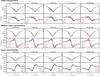 |
Fig. 13. Profiles coming from the pixels marked in Fig. 12 (black dots). For visualization purposes, I profiles are normalized by the percentage of scans involved in the signal addition. Curves in violet, orange, and red stand for the δI(λ)/δλ scaled by −CB∥ for Δλ1, Δλ2, and Δλ3, respectively. The corresponding B∥ values are indicated in G following the same color scheme. Profiles from the M datasets are shown by dashed gray lines. |
Statistics on the chromospheric and photospheric magnetic flux in the depicted field concentrations using the NM datasets.
Finally, Fig. 14 shows the histograms of the number of pixels with two-lobed V profiles in the concentrations analyzed using the NM datasets and their B∥ values for each spectral range. The former distributions are normalized to the number of scans showing each group whereas the latter are normalized to the number of pixels per group in all sequences (∼46×103, 150×103, and 510×103 pixels for small, medium-sized, and large structures), respectively. Although all distributions resemble those for the M datasets (Fig. 2), they are affected by the value smearing, as fewer pixels meet the threshold used to delimit each case (Fig. 14a) and the peaks of some distributions are shifted to stronger estimates (Figs. 14b–d).
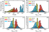 |
Fig. 14. Histograms of the number of pixels with two-lobed Stokes V signals (panel a) and B∥ values for Δλ1, Δλ2, and Δλ3 (panels b–d) in the studied cases using the NM datasets. Yellow, red, and blue distributions represent pixels in small, medium-sized, and large field concentrations, respectively. The upper-left corner of the panels show the median value of each distribution. |
5.2. Comparison with previous studies
Over the past few years, investigations based on high-spatial-resolution data have reported a weakening of the quiet-Sun magnetic fields with height (e.g., Gošić et al. 2018; Robustini et al. 2019; Morosin et al. 2020). We also observe a transition to weaker longitudinal fields as the spectral range narrows down around the line core.
Close to the limb, Robustini et al. (2019) found longitudinal magnetic fields of ∼400 G in the photosphere decreasing to 200 G in the chromosphere of quiet-Sun areas. To estimate the latter, these authors applied the WFA to a spectral range of ±1 Å from the Ca II 854.2 nm line center. At a heliocentric angle of 37°, Pietrow et al. (2020) inferred B∥ values of about 250 G outside a plage by performing STiC inversions of full-Stokes data in the λ8542 line (sampled within ±880 mÅ from the line center). Also outside a plage but closer to the disk center, Morosin et al. (2020) reported a weakening of B∥ from ∼−600 G in the photosphere to −200 G in the low-mid chromosphere by applying a spatially constrained WFA method to the wings of the Na I 589.6 nm line and the Ca II 854.2 nm core (±110 mÅ). Recently, Gošić et al. (2021) found maximum B∥ values of 400–800 G in internetwork clusters in Fe I 617.3 nm data that weaken by more than 200 G when applying the WFA to a spectral range of ±200 mÅ in the Ca II 854.2 nm line core.
We report B∥ values of hG in quiet-Sun magnetic concentrations. Our mostly photospheric and chromospheric estimates in small and medium-sized structures are compatible with those previously found. However, our results for wider ranges across the line are stronger. Large concentrations also show stronger estimates, which is likely due to a departure of their physical properties from those typically found in the quiet Sun. Finally, we note that differences in the heliocentric angle may also lead to divergence of the results from those of other studies.
Furthermore, an interesting aspect of our study is the comparison of the photospheric and chromospheric estimates in concentrations of different size. Small concentrations usually host compact height variations of B∥ exceeding 400–500 G, where the maximum can be stronger than 800 G. Medium-sized and large structures show similar height variations but more extended over the concentrations. However, inspection of the average height variation of B∥ reveals that small and medium-sized concentrations have stronger average height variation (of about 400 and 425 G, respectively) than large concentrations (of ∼300 G). Corroborating this result by analyzing other large concentrations will be of great interest because our sample only has two large structures, which were observed under poor seeing conditions. In addition, the height variations of B∥ can be considered weaker or stronger than the chromospheric B∥ estimated in each structure. In this regard, when compared to large concentrations, small and medium-sized concentrations display stronger height gradients in B∥ than their chromospheric estimates. Consequently, large structures usually show better fits between the observed V profiles and the scaled I derivatives for wider spectral ranges.
Investigations of the stratification of the magnetic field with height in sunspots have revealed discrepancies depending on the approach used to determine the magnetic gradients (see the review of Balthasar 2018). Undoubtedly, similar studies in the quiet Sun are also of great importance as they can shed light on the topology of its magnetic field. Nonetheless, the elusive detection of the weak polarization signals emerging from the quiet-Sun chromosphere hinders these investigations. This impasse will be overcome by using observations acquired with the next-generation solar telescopes, such as DKIST (Rimmele et al. 2020) and EST (Quintero Noda et al. 2022).
6. Conclusions and summary
Characterization of the magnetic field of the quiet-Sun chromosphere is essential for comprehending the chromospheric heating and the coupling of the magnetic field between the photosphere and the outer atmosphere. For this reason, we determined the longitudinal component of the magnetic field inferred in quiet-Sun magnetic concentrations depending on their size. Specifically, we applied the WFA to high-spatial-resolution Ca II 854.2 nm data acquired close to the disk center with SST/CRISP using different spectral ranges and temporally combined signals.
We find a correlation between the amplitude of B∥ estimates and concentration size, with large structures hosting the largest values of B∥. By restricting the spectral range to the line core, we infer chromospheric estimates that smoothly change from ∼50 at the edges to 150–500 G at the center of the concentrations. These values increase as the spectral range widens due to the influence of the photospheric contribution, which is especially strong compared to the chromospheric estimates in small and medium-sized concentrations. Consequently, the photospheric magnetic flux is three to four times greater than the chromospheric one in the large concentration and this difference can be as large as one order of magnitude in the small and medium-sized cases.
The effect of the height gradients in B∥ on the reliability of the estimates given by the WFA depends on the concentration size and spectral range. Estimates for the inner-core range are usually reliable regardless of the concentration size, though they are affected by relative shifts between the I and V signals at some locations. In contrast, estimates for wider spectral ranges are generally unreliable in small and medium-sized structures.
Although differences in B∥ and size are seen in small concentrations due to their dynamic behavior, signal addition usually leads to estimates akin to those at the original cadence for all spectral ranges. Therefore, we infer that the conditions along the considered formation regions may be stable with time in the studied structures and that signal addition has not warranted the detection of weaker signals. Moreover, signal addition reduces the noise of the chromospheric estimates and is not related to a better fulfillment of the WFA requisites when using wider ranges.
Finally, although deconvolving processes may enhance noise levels, data restored by destretching show similar results to those obtained when using the MOMFBD technique. However, results from the former are affected by the smearing caused by the partial correction of the data.
Movies
Movie 1 associated with Fig. 3 Access Supplementary Material
Movie 2 associated with Fig. 7 Access Supplementary Material
Movie 3 associated with Fig. 10 Access Supplementary Material
Acknowledgments
We thank the technical support provided by Dr. Ángel de Vicente. We acknowledge the funding received from the European Research Council (ERC) under the European Union’s Horizon 2020 research and innovation program (ERC Advanced Grant agreement No. 742265), as well as from the Spanish Ministerio de Ciencia, Innovación y Universidades through project PGC2018-102108-B-I00 and FEDER funds. This project has received funding also from the European Research Council (ERC) under the European Union’s Horizon 2020 research and innovation programme (SUNMAG, grant agreement 759548). The Swedish 1-m Solar Telescope is operated on the island of La Palma by the Institute for Solar Physics of Stockholm University in the Spanish Observatorio del Roque de los Muchachos of the Instituto de Astrofísica de Canarias. The Institute for Solar Physics is supported by a grant for research infrastructures of national importance from the Swedish Research Council (registration number 2017-00625). This research has made use of NASA’s Astrophysical Data System.
References
- Afonso Delgado, D., del Pino Alemán, T., & Trujillo Bueno, J. 2023, ApJ, 942, 60 [NASA ADS] [CrossRef] [Google Scholar]
- Asensio Ramos, A., Martínez González, M. J., López Ariste, A., Trujillo Bueno, J., & Collados, M. 2007, ApJ, 659, 829 [Google Scholar]
- Auer, L. H., & Heasley, J. N. 1978, A&A, 64, 67 [NASA ADS] [Google Scholar]
- Balthasar, H. 2018, Sol. Phys., 293, 120 [NASA ADS] [CrossRef] [Google Scholar]
- Bellot Rubio, L., & Orozco Suárez, D. 2019, Liv. Rev. Sol. Phys., 16, 1 [Google Scholar]
- Carlin, E. S., & Asensio Ramos, A. 2015, ApJ, 801, 16 [NASA ADS] [CrossRef] [Google Scholar]
- Cauzzi, G., Reardon, K. P., Uitenbroek, H., et al. 2008, A&A, 480, 515 [NASA ADS] [CrossRef] [EDP Sciences] [Google Scholar]
- Centeno, R. 2018, ApJ, 866, 89 [Google Scholar]
- Centeno, R., Socas-Navarro, H., Lites, B., et al. 2007, ApJ, 666, L137 [CrossRef] [Google Scholar]
- Danilovic, S., van Noort, M., & Rempel, M. 2016, A&A, 593, A93 [NASA ADS] [CrossRef] [EDP Sciences] [Google Scholar]
- de la Cruz Rodríguez, J., Socas-Navarro, H., Carlsson, M., & Leenaarts, J. 2012, A&A, 543, A34 [Google Scholar]
- de la Cruz Rodríguez, J., Rouppe van der Voort, L., Socas-Navarro, H., & van Noort, M. 2013, A&A, 556, A115 [NASA ADS] [CrossRef] [EDP Sciences] [Google Scholar]
- de la Cruz Rodríguez, J., Löfdahl, M. G., Sütterlin, P., Hillberg, T., & Rouppe van der Voort, L. 2015, A&A, 573, A40 [NASA ADS] [CrossRef] [EDP Sciences] [Google Scholar]
- de la Cruz Rodríguez, J., Leenaarts, J., Danilovic, S., & Uitenbroek, H. 2019, A&A, 623, A74 [Google Scholar]
- Esteban Pozuelo, S., de la Cruz Rodríguez, J., Drews, A., et al. 2019, ApJ, 870, 88 [Google Scholar]
- Fontenla, J. M., Avrett, E. H., & Loeser, R. 1993, ApJ, 406, 319 [Google Scholar]
- Gömöry, P., Balthasar, H., & Puschmann, K. G. 2013, A&A, 556, A7 [NASA ADS] [CrossRef] [EDP Sciences] [Google Scholar]
- Gošić, M., Bellot Rubio, L. R., Orozco Suárez, D., Katsukawa, Y., & del Toro Iniesta, J. C. 2014, ApJ, 797, 49 [Google Scholar]
- Gošić, M., de la Cruz Rodríguez, J., De Pontieu, B., et al. 2018, ApJ, 857, 48 [CrossRef] [Google Scholar]
- Gošić, M., De Pontieu, B., Bellot Rubio, L. R., Sainz Dalda, A., & Esteban Pozuelo, S. 2021, ApJ, 911, 41 [CrossRef] [Google Scholar]
- Hotelling, H. 1933, J. Educ. Psychol., 24, 417 [CrossRef] [Google Scholar]
- Illing, R. M. E., Landman, D. A., & Mickey, D. L. 1975, A&A, 41, 183 [NASA ADS] [Google Scholar]
- Jennerholm Hammar, F. 2014, Master’s Thesis, Uppsala Universitet, Sweden [Google Scholar]
- Kalkofen, W. 1989, ApJ, 346, L37 [NASA ADS] [CrossRef] [Google Scholar]
- Khomenko, E., & Collados, M. 2012, ApJ, 747, 87 [Google Scholar]
- Khomenko, E. V., Collados, M., Solanki, S. K., Lagg, A., & Trujillo Bueno, J. 2003, A&A, 408, 1115 [NASA ADS] [CrossRef] [EDP Sciences] [Google Scholar]
- Landi Degl’Innocenti, E., & Landolfi, M. 2004, Polarization in Spectral Lines, 307 (Dordrecht: Kluwer Academic Publishers) [Google Scholar]
- Leenaarts, J., de la Cruz Rodríguez, J., Kochukhov, O., & Carlsson, M. 2014, ApJ, 784, L17 [NASA ADS] [CrossRef] [Google Scholar]
- Livingston, W. C., & Harvey, J. 1975, Bull. Am. Astron. Soc., 7, 346 [Google Scholar]
- Löfdahl, M. G., & Scharmer, G. B. 1994, A&AS, 107, 243 [NASA ADS] [Google Scholar]
- Löfdahl, M. G., Hillberg, T., de la Cruz Rodríguez, J., et al. 2021, A&A, 653, A68 [Google Scholar]
- Manso Sainz, R., & Trujillo Bueno, J. 2010, ApJ, 722, 1416 [NASA ADS] [CrossRef] [Google Scholar]
- Martínez González, M. J., & Bellot Rubio, L. R. 2009, ApJ, 700, 1391 [CrossRef] [Google Scholar]
- Martínez González, M. J., Collados, M., Ruiz Cobo, B., & Solanki, S. K. 2007, A&A, 469, L39 [NASA ADS] [CrossRef] [EDP Sciences] [Google Scholar]
- Martínez González, M. J., Manso Sainz, R., Asensio Ramos, A., & Bellot Rubio, L. R. 2010, ApJ, 714, L94 [CrossRef] [Google Scholar]
- Morosin, R., de la Cruz Rodríguez, J., Vissers, G. J. M., & Yadav, R. 2020, A&A, 642, A210 [NASA ADS] [CrossRef] [EDP Sciences] [Google Scholar]
- Morosin, R., de la Cruz Rodríguez, J., Díaz Baso, C. J., & Leenaarts, J. 2022, A&A, 664, A8 [NASA ADS] [CrossRef] [EDP Sciences] [Google Scholar]
- Ortiz, A., Bellot Rubio, L. R., Hansteen, V. H., de la Cruz Rodríguez, J., & Rouppe van der Voort, L. 2014, ApJ, 781, 126 [NASA ADS] [CrossRef] [Google Scholar]
- Pearson, K. 1901, Phil. Mag., 6, 559 [CrossRef] [Google Scholar]
- Pietrow, A. G. M., Kiselman, D., de la Cruz Rodríguez, J., et al. 2020, A&A, 644, A43 [NASA ADS] [CrossRef] [EDP Sciences] [Google Scholar]
- Priest, E. R., Chitta, L. P., & Syntelis, P. 2018, ApJ, 862, L24 [Google Scholar]
- Puschmann, K. G., & Beck, C. 2011, A&A, 533, A21 [NASA ADS] [CrossRef] [EDP Sciences] [Google Scholar]
- Quintero Noda, C., Shimizu, T., de la Cruz Rodríguez, J., et al. 2016, MNRAS, 459, 3363 [Google Scholar]
- Quintero Noda, C., Schlichenmaier, R., Bellot Rubio, L. R., et al. 2022, A&A, 666, A21 [NASA ADS] [CrossRef] [EDP Sciences] [Google Scholar]
- Rimmele, T. R., Warner, M., Keil, S. L., et al. 2020, Sol. Phys., 295, 172 [Google Scholar]
- Robustini, C., Esteban Pozuelo, S., Leenaarts, J., & de la Cruz Rodríguez, J. 2019, A&A, 621, A1 [NASA ADS] [CrossRef] [EDP Sciences] [Google Scholar]
- Sánchez Almeida, J., & Martínez González, M. 2011, ASP Conf. Ser., 437, 451 [Google Scholar]
- Scharmer, G. B. 2006, A&A, 447, 1111 [NASA ADS] [CrossRef] [EDP Sciences] [Google Scholar]
- Scharmer, G. B., Bjelksjo, K., Korhonen, T. K., Lindberg, B., & Petterson, B. 2003, SPIE, 4853, 341 [Google Scholar]
- Scharmer, G. B., Narayan, G., Hillberg, T., et al. 2008, ApJ, 689, L69 [Google Scholar]
- Schrijver, C. J., & Title, A. M. 2003, ApJ, 597, L165 [NASA ADS] [CrossRef] [Google Scholar]
- Sheeley, N. R., Jr., 1967, Sol. Phys., 1, 171 [NASA ADS] [CrossRef] [Google Scholar]
- Smithson, R. C. 1975, Bull. Am. Astron. Soc., 7, 346 [Google Scholar]
- Spruit, H. C. 1976, Sol. Phys., 50, 269 [NASA ADS] [CrossRef] [Google Scholar]
- Trujillo Bueno, J., Shchukina, N., & Asensio Ramos, A. 2004, Nature, 430, 326 [Google Scholar]
- Trujillo Bueno, J., Asensio Ramos, A., & Shchukina, N. 2006, ASP Conf. Ser., 358, 269 [NASA ADS] [Google Scholar]
- Uitenbroek, H. 2006, ASP Conf. Ser., 354, 313 [NASA ADS] [Google Scholar]
- van Noort, M., Rouppe van der Voort, L., & Löfdahl, M. G. 2005, Sol. Phys., 228, 191 [Google Scholar]
- van Noort, M. J., & Rouppe van der Voort, L. H. M. 2008, A&A, 489, 429 [NASA ADS] [CrossRef] [EDP Sciences] [Google Scholar]
- Vissers, G., & Rouppe van der Voort, L. 2012, ApJ, 750, 22 [Google Scholar]
- Zirin, H. 1985, Aust. J. Phys., 38, 961 [NASA ADS] [CrossRef] [Google Scholar]
All Tables
Heliocentric coordinates of the FOV center at the beginning of the observing run, time interval, and number of scans of each dataset.
Statistics on the chromospheric and photospheric magnetic flux in the depicted field concentrations.
Statistics on the chromospheric and photospheric magnetic flux in the depicted field concentrations using the NM datasets.
All Figures
|
Fig. 1. Intensity filtergrams of the Ca II 854.2 nm line core and at −1.755 Å (left and middle columns), and blue-wing magnetograms of Ca II 854.2 nm at −0.39 Å from the line center (right column). The red rectangles show the positions of the analyzed structures. The time stamp of each scan in UT is shown in the upper-left corner labels. Axes are labeled in arcseconds. |
| In the text | |
|
Fig. 2. Histograms of the number of pixels with two-lobed Stokes V signals (panel a), and B∥ values for Δλ1, Δλ2, and Δλ3 (panels b–d) in the studied cases. Distributions of pixels within small, medium-sized, and large field concentrations are colored in yellow, red, and blue, respectively. The median value of each distribution is shown in the upper-left corner of the panels. |
| In the text | |
|
Fig. 3. Magnetograms at −0.39 Å and B∥ estimates on a small field concentration at different Δt. Left: Ca II 854.2 nm intensity filtergram at −1.755 Å. The yellow rectangle encloses the region shown on the right-hand side. Right (from top to bottom): blue-wing magnetograms at −0.39 Å and B∥ estimates from Δλ1, Δλ2, and Δλ3. Pink contours delimit the structure, black ones enclose pixels with two-lobed V signals inside it. The plus symbols (+) and crosses (×) mark the pixels shown in the two upper and lower rows of Fig. 4, respectively. Major tick marks represent 1″. A movie showing the temporal evolution of the parameters displayed in this figure is available online. |
| In the text | |
|
Fig. 4. Stokes I and V profiles emerging from a small concentration for different Δt (black dots). For visualization purposes, intensity profiles are normalized by the percentage of scans involved in the signal addition. Violet, orange, and red curves stand for the δI(λ)/δλ functions scaled by −CB∥ for Δλ1, Δλ2, and Δλ3, respectively. B∥ values for Δλ1, Δλ2, and Δλ3 in G are shown on each panel in violet, orange, and red. |
| In the text | |
|
Fig. 5. Synthetic V profiles computed from different gradients in B∥ between log(τ500) = 1.3 and −5.3: from 1000 to 100 G (panel a) and from 300 to 100 G (panel b). The dashed gray lines mark the V values at the first and last wavelength positions, and the dotted gray lines indicate zero polarization signal. |
| In the text | |
|
Fig. 6. Chromospheric and photospheric estimates in the small concentration at the original cadence (panels a and b), and temporal evolution of the corresponding magnetic flux (panel c). Major tick marks represent 1″. Black contours enclose pixels with two-lobed V profiles. We note that the values represented in panels a and b are saturated using different scales, which range from 0 to 175 G and from 100 to 1000 G, respectively. |
| In the text | |
|
Fig. 7. Magnetograms at −0.39 Å and B∥ maps on a medium-sized concentration for different Δt. The plus symbols (+) and crosses (×) mark the pixels displayed in the two upper and lower rows of Fig. 8, respectively. Same layout as in Fig. 3. An animated version of this figure displaying the temporal evolution of this case is available online. |
| In the text | |
|
Fig. 8. Stokes I and V profiles coming from the depicted medium-sized concentration for different Δt, and their comparison to the Stokes I derivatives scaled by −CB∥ for Δλ1, Δλ2, and Δλ3, respectively. Same layout as in Fig. 4. |
| In the text | |
|
Fig. 9. Chromospheric and photospheric B∥ estimates in the medium-sized case at the original cadence (panels a and b), and temporal evolution of the corresponding magnetic flux (panel c). Major tick marks represent 1″. Black contours enclose pixels with two-lobed V profiles. We note that the values represented in panels a and b are saturated using different scales, which range from 0 to 400 G and from 100 to 1200 G, respectively. |
| In the text | |
|
Fig. 10. Magnetograms at −0.39 Å and B∥ estimates on a large concentration for different Δt. The plus symbols (+) and crosses (×) mark the pixels shown in the two upper and lower rows of Fig. 11, respectively. The yellow rectangle delimits the region displayed on the right-hand side. Same layout as in Fig. 3. A movie showing the temporal evolution of the parameters displayed in this figure is available online. |
| In the text | |
|
Fig. 11. Stokes I and V profiles coming from the depicted large concentration at different Δt, and their comparison to the Stokes I derivatives scaled by −CB∥ for Δλ1, Δλ2, and Δλ3, respectively. Same layout as in Fig. 4. |
| In the text | |
|
Fig. 12. Details of the cases shown in Figs. 3, 7, and 10 using the NM datasets. Left: Ca II 854.2 nm intensity filtergrams at −1.755 Å. The yellow rectangles superimposed over the small and large concentrations enclose the regions shown zoomed-in on the right-hand side. Right: magnetograms at −0.39 Å and B∥ estimates for each Δλ and Δt. The plus symbols (+) mark the pixels shown in Fig. 13. Pink and black contours enclose each case and the pixels with two-lobed V profiles inside them, respectively. Major tick marks represent 1″. |
| In the text | |
|
Fig. 13. Profiles coming from the pixels marked in Fig. 12 (black dots). For visualization purposes, I profiles are normalized by the percentage of scans involved in the signal addition. Curves in violet, orange, and red stand for the δI(λ)/δλ scaled by −CB∥ for Δλ1, Δλ2, and Δλ3, respectively. The corresponding B∥ values are indicated in G following the same color scheme. Profiles from the M datasets are shown by dashed gray lines. |
| In the text | |
|
Fig. 14. Histograms of the number of pixels with two-lobed Stokes V signals (panel a) and B∥ values for Δλ1, Δλ2, and Δλ3 (panels b–d) in the studied cases using the NM datasets. Yellow, red, and blue distributions represent pixels in small, medium-sized, and large field concentrations, respectively. The upper-left corner of the panels show the median value of each distribution. |
| In the text | |
Current usage metrics show cumulative count of Article Views (full-text article views including HTML views, PDF and ePub downloads, according to the available data) and Abstracts Views on Vision4Press platform.
Data correspond to usage on the plateform after 2015. The current usage metrics is available 48-96 hours after online publication and is updated daily on week days.
Initial download of the metrics may take a while.