| Issue |
A&A
Volume 671, March 2023
|
|
|---|---|---|
| Article Number | A23 | |
| Number of page(s) | 16 | |
| Section | Planets and planetary systems | |
| DOI | https://doi.org/10.1051/0004-6361/202245023 | |
| Published online | 02 March 2023 | |
Semi-automatic meteoroid fragmentation modeling using genetic algorithms
Astronomical Institute, Czech Academy of Sciences,
Fričova 298,
251 65
Ondřejov, Czech Republic
e-mail: ftom@physics.muni.cz
Received:
20
September
2022
Accepted:
19
January
2023
Context. Meteoroids are pieces of asteroids and comets. They serve as unique probes to the physical and chemical properties of their parent bodies. We can derive some of these properties when meteoroids collide with the atmosphere of Earth and become a meteor or a bolide. Even more information can be obtained when meteoroids are mechanically strong and slow enough to drop meteorites.
Aims. Through physical modeling of bright meteors, we describe their fragmentation in the atmosphere. We also derive their mechanical strength and the mass distribution of the fragments, some of which may hit the ground as meteorites.
Methods. We developed a semi-automatic program for meteoroid fragmentation modeling using parallel genetic algorithms. This allowed us to determine the most probable fragmentation cascade of the meteoroid, and also to specify its initial mass and velocity. These parameters can be used in turn to derive the heliocentric orbit of the meteoroid and to place constraints on its likely age as a separate object.
Results. The program offers plausible solutions for the majority of fireballs we tested, and the quality of the solutions is comparable to that of manual solutions. The two solutions are not the same in detail, but the derived quantities, such as the fragment masses of the larger fragments and the proxy for their mechanical strength, are very similar. With this method, we would like to describe the mechanical properties and structure of both meteoroids belonging to major meteor showers and those that cause exceptional fireballs.
Key words: meteorites, meteors, meteoroids / Earth / methods: numerical
© The Authors 2023
 Open Access article, published by EDP Sciences, under the terms of the Creative Commons Attribution License (https://creativecommons.org/licenses/by/4.0), which permits unrestricted use, distribution, and reproduction in any medium, provided the original work is properly cited.
This article is published in open access under the Subscribe to Open model. Subscribe to A&A to support open access publication.
1 Introduction
Meteoroids are fragments of comets and asteroids. They are therefore a valuable source of information about those objects. Observations of meteoroids can provide us with clues about their structure, density, and mechanical strength. If they produce meteorites, we can also derive their porosity, mineralogy, and chemical composition, and all sorts of other physical properties. Meteorite-producing fireballs are also a very rare opportunity for a cheap sampling of material from asteroids, which greatly increases the scientific return of their observations.
Research of asteroids and comets brings a wealth of information about the physical and chemical properties of the protosolar nebula. These bodies also provide constraints on the process of formation and the following evolution of the Solar System. Moreover, revealing the history of our Solar System enables important insights into the formation and evolution of other planetary systems, including the formation of planets similar to our Earth that can potentially host life.
Moreover, even small asteroids pose a threat to life on Earth, as was demonstrated, for example, in February 2013 by the Chelyabinsk meteorite fall (Borovička et al. 2013a; Brown et al. 2013; Popova et al. 2013). This event caused many injuries, and more than 1600 people sought medical help in hospitals (Akimov et al. 2015; Kartashova et al. 2018). It served as a warning sign and a reminder that asteroid and fireball observations are also important in the context of planetary defense. These observations allow us to calculate the likelihood of being hit by a projectile of a certain size more precisely, and they enable us to estimate the possible outcomes of such a collision for our civilization as well as the environment.
Many characteristics of a meteoroid can easily be derived from the fireball observations, but some parameters are dependent on detailed physical modeling and comparison with all the available observations. Classical models include those reported by Baldwin & Sheaffer (1971) and Hills & Goda (1993). Hydro-dynamical modeling of outcomes of the comet Shoemaker-Levy 9 impact on Jupiter was reported by Ahrens et al. (1994) and Boslough et al. (1994). The disintegration of larger meteoroids and asteroids in the atmosphere of Earth was modeled by Svetsov et al. (1995). A more recent fragment-cloud model of the asteroid atmospheric breakup and energy deposition was introduced in Wheeler et al. (2017) and was extended and evaluated for various internal structures of meteorids by Wheeler et al. (2018). A recent detailed review of various approaches to meteoroid entry modeling is given in Popova et al. (2019).
Our paper extends the modeling efforts of Borovička et al. (2013b), who successfully modeled the Košice meteorite fall with their semi-empirical model. They were not only able to predict very precisely where the meteorites would be found, but also described the fireball phenomenon in great detail. That modeling also included the effect of the so-called erosion, which was previously used for the successful modeling of Draconid meteors (Borovička et al. 2007). Further improvements of the model are reflected in the recent paper of Borovička et al. (2020).
The main goal of these modeling efforts is to find a precise initial mass and velocity of the meteoroid, fragmentation times that enable us to derive the bulk strength of a fragmenting body, the number and physical properties of daughter fragments that originated in the meteoroid fragmentation cascade, and the mass distribution of the dust particles. Moreover, in some exceptional cases, we would like to derive the masses and distribution of potential meteorites after additional modeling of the dark flight. In other words, we are interested in the internal structure and also in the mass and strength distributions of the meteoroid and its constituents.
The trial-and-error method of Borovička et al. (2020) was used for manual modeling with the Firmodel program. It produces a good eyeball fit of the radiometric curve, the photometric light curve, and the dynamics of the fireball.
The manual approach, however, is time-consuming, and it searches the parametric space of the problem randomly. The solution may not be unique, and some better solutions that are not found in this way may even exist. Therefore, we develop a semi-automatic modeling procedure that searches the parametric space more thoroughly and can find more solutions that can then be compared. The best solution can finally be chosen.
The European Fireball Network (EN) has provided observations of fireballs over Central Europe for decades. It is being actively developed and expanded by new stations and new instrumentation (Spurný et al. 2007, 2017). Because the sky is monitored for bright fireballs every night, and because the observing methods are gradually improved and even expanded, the number of high-quality observations is ever-growing. The processing of the raw data is now well established, and the only remaining step toward deriving meteoroid physical characteristics is data modeling.
When developing the semi-automatic modeling procedure, our first idea was to search the parametric space as thoroughly as possible. However, because the problem is so complex, the parametric space is vast. No traditional method would complete the search in a reasonable time, and/or a traditional method would probably only find some local optimum. Therefore, we envisioned a semi-automatic approach to the problem by the use of parallel genetic algorithm (GA) optimization. In this way, it should be possible to find a solution that optimizes all data of the fireball (radiometric and photometric light curves, and dynamics), and this solution may also be similar to a manual solution of the problem. Tárano et al. (2019) were the first who used the combination of a GA optimizer with a meteoroid fragmentation model, namely the fragment-cloud model of Wheeler et al. (2017), to derive the physical characteristics of meteoroids. Later, Tárano (2020) expanded this work by using supervised learning methods and suggested further improvements of the meteoroid characteristics inference.
Compared to Tárano et al. (2019), there are several important differences. First, our luminous efficiency is not a constant, but a function that depends on both the mass and the velocity of the meteoroid. Second, we can calculate the meteoroid initial velocity and height from the dynamics data alone, while the initial (photometric) mass is estimated from the radiometric curve. All of these values are then optimized while the solution is found, but the initial estimates dramatically shrink the search space. Third, we optimize three separate datasets: radiometric and photometric light curves, and dynamics. These data carry more detailed information about the meteoroid entry than the energy deposition curve that was used in Tárano et al. (2019) and other studies. Fourth, we use a different fragmentation model that is more driven by the data itself, that is, fragmentation times are deduced from the radiometric curve and are verified by the dynamics. Further details can be found below in Sect. 3.
The algorithm extensively uses pseudo-random numbers at the initialization and during the calculation to choose the values of the free parameters. From the previous use of GA, we know that it can converge to a global optimum of the problem. Therefore, the algorithm is probably capable of finding a unique set of solutions for the fireball fragmentation in the atmosphere as well. We expect that there will be several solutions to the problem with a similar quality that may differ in details or differ even more substantially. When we obtain these solutions, we can compare them and determine the best of them, or we can define what a general solution looks like. These solutions may differ in the particular number of fragments, their respective masses, and other parameters. Nevertheless, we should be able to find a plausible range of these values. If we succeed in finding the global optimum of the problem, we can then calculate the uncertainties of the fit by inspecting its close vicinity by a systematic search or by a Monte Carlo method.
Section 2 contains the description of observation methods and data processing, and Sect. 3 introduces FirMpik, the semi-automatic program for data modeling. In Sect. 4, and in Appendix A we summarize our results, which we discuss in Sect. 5, and Sect. 6 lists our main conclusions and future plans.
2 Data and their modeling
2.1 Observations
All the modeled data come from the European fireball network, which comprises 21 stations in central Europe: 15 stations are in the Czech Republic, 4 in Slovakia, and one each in Austria and in Germany. These stations are equipped with the Digital Autonomous Fireball Observatory, or DAFO, which has been developed at the Astronomical Institute of The Czech Academy of Sciences in Ondrejov. The observatory contains two digital all-sky cameras and a sensitive photomultiplier tube pointed toward the zenith that produces very precise hightime-resolution radiometric data. Some stations also contain narrow-field cameras for detailed observations of meteoroid fragmentation. The fireball trail in the all-sky image is interrupted by an LCD shutter behind the lens with a frequency of 16 Hz (this can be modified remotely) to enable a measurement of the fireball velocity. For temporal calibration, one interruption is omitted every whole second, producing a longer dash on the fireball trail. Time at respective stations is continuously corrected by the pulse-per-second (PPS) signal of the GPS, providing an absolute timing error better than 1 µs. Because all the data are digital, they are daily uploaded to a central server and are immediately available. The data are preprocessed, and bright fireballs are automatically detected, which enables a timely modeling.
2.2 Data reduction
The data on the brightest fireballs are reduced on the day after the observations. The radiometric curve is calibrated to absolute magnitudes (fireball brightness at a 100 km distance from the station) by comparison with digital photographs from all-sky cameras. The all-sky image with a captured fireball is calibrated both astrometrically and photometrically, and then the positions and brightness of individual parts of the trail are measured. These measurements with time calibrations produce a light curve that provides valuable information of the fainter parts of the fireball (the beginning and the end) because the radiometer is less sensitive than the digital camera. On the other hand, the radiometer has a much wider dynamic range than the camera. Fireball observations from two or more stations enable us to calculate its trajectory in the atmosphere. The dynamics of the foremost meteoroid fragment, or its length along the trajectory versus time, is calculated from the position measurements of individual breaks of the fireball trail caused by the LCD shutter (Borovička et al. 2020).
2.3 Modeling
In the original version of the Firmodel program, the modeling is performed in a trial-and-error fashion. The user fits the data by eye, in other words, there is no objective measure of the fit in the process, although the fit is checked in the O–C plot. This plot shows the difference between the observed (O) and calculated (C) values of the length along the trajectory of the fireball (length residuals) or the fireball brightness measured from the all-sky images or by a radiometer as a function of time or height above the ground. The automatic algorithm we developed also uses a trial-and-error method together with simplified but very powerful rules of natural selection, inheritance, and variation. As a fitness function (an objective function specific for GA, opposite of the cost function) that measures the quality of each solution, we use the inverse value of the reduced χ2 sum of the model fit to all available data. The reduced χ2 is defined as
 (1)
(1)
where wrlc, wlc, and wlen denote the weights of the three datasets we use in finding the fragmentation model (more details are given in Sect. 3.11), Ndata is the total number of datapoints, and Nparm is the number of free parameters sought in the modeling. The respective contributions to the total χ2 sum from the three datasets are calculated as
 (2)
(2)
 (3)
(3)
 (4)
(4)
Here wfrag refers to the weights used to emphasize the importance of fragmentations in the radiometric curve (see details in Sect. 3.13), rlcsmooth is the measured brightness from the median-smoothed radiometric curve, σrlc is the intrinsic uncertainty of the brightness measured by the radiometer, Mmodel is the total brightness calculated from the model, lc is the fireball brightness measured from the all-sky image for individual breaks, σlc is the brightness intrinsic uncertainty, len is the measured length of the leading fragment, and Lmodel is its calculated length. No uncertainty is related to the measured length, and it is therefore not part of our calculations. The datapoint uncertainties (more precisely, 1/σ2) serve as weights to emphasize the effect of datapoints with a lower uncertainty on the overall χ2 sum and reduce the effect of datapoints with a higher uncertainty. The weights for length datapoints are all set to one.
All the sum symbols imply summing over all datapoints in the respective datasets. Because the model is calculated with a finite time resolution, the values used to compute the χ2 sum are linearly interpolated for the exact time instants of observations. Because the problem we model is highly nonlinear and also because of the weights used in the calculation, the χ2 does not have a strict statistical meaning, but rather serves as a relative measure of the goodness of fit. This also has implications for the confidence intervals of the quantities found by the modeling. In a typical optimization run, the value of the fitness function grows very fast at the beginning, curves over later in the process, and reaches a plateau with an occasional sudden rise.
The data for the radiometric curve are very precise (except for the beginning and end of the curve, because the signal-to-noise ratio is low), and the data from different observing stations are clearly related. Still, we observe some spread in the brightness values that are due to varying properties of radiometers and different weather conditions. Therefore, the user who determines the model manually can use this spread to hide some minor fragmentations that optimize both the radiometric data and dynamics. In contrast, the automatic fitting algorithm uses an objective measure (the reduced χ2 sum with respect to the smoothed radiometric curve, light curve, and dynamic data) and any departure from these data is penalized by an increase in the χ2 sum. It is therefore more critical to find the fragmentations in the radiometric curve as reliably as possible so that the fit can optimize all the available data.
The user who fits the fireball data manually also has more information about the data quality. The radiometric data have intrinsic uncertainties that are used for the χ2 sum calculation. The uncertainties reflect objective observational conditions at the respective station, but some problem with the data may occasionally be hidden that does not propagate to its uncertainties. The user can check the suspect data (which are poorly fit by the model) and decide to ignore them or give them a lower priority while constructing the model. The automatic algorithm, however, does not have this additional information. Moreover, the dynamic data have no a priori uncertainties whatsoever. The model also assumes a steady-state ablation, which is not satisfied at the beginning of the observation when the meteoroid is gradually heated up and only starts to shine. The brightness of the fireball as predicted by the model is then higher than observed. This means that even though the automatic algorithm computes the reduced χ2 value for every solution, it mainly serves as a relative measure of the fit quality. A solution is accepted when the overall quality of the fit to all the datasets by a model is good enough as judged by the user, not only by the χ2 sum.
3 FirMpik program
FirMpik is a global optimization program for semi-automatic modeling of fireball fragmentation in the atmosphere. It uses GA to search for several tens of parameters describing the ablation, radiation, and fragmentation of a meteoroid during the visible flight. These parameters include the number of fragments released from their respective parents in gross fragmentation events, their respective masses, whether or not the fragment erodes, and if it does, the erosion coefficient, and the mass distribution limits of dust in both the gross and continuous fragmentations. The model is created for the whole observation dataset at once, and it is compared by means of reduced χ2 statistics to all the data that are available for a specific fireball observation. These data are comprised of the radiometric light curve taken by a sensitive photomultiplier tube pointed to the zenith, optical light curve and dynamic data measured from images taken by digital all-sky cameras, and occasionally, also individual fragment observations from narrow-field cameras placed on several stations of the Czech part of the EN. FirMpik uses the same fragmentation model as the Firmodel program.
3.1 Firmodel program
Firmodel is a computer program developed by Jiří Borovička that is used for the manual modeling of atmospheric fragmentation of meteoroids. It was first used to model the Košice meteorite fall (Borovička et al. 2013b). The model is described in great detail in Borovička et al. (2020); we describe the model briefly below.
The fragmentation model used in the Firmodel program is semi-empirical in the sense that the fragmentation times have to be determined in the modeling process from the observed data of the modeled fireball. These comprise a radiometric curve, a photometric light curve, and dynamics. The radiometric curve of most fireballs contains very fast semi-periodic brightness changes. They might be caused by an instability of ablation, but the present model does not account for these brightness changes. Therefore, in modeling the bolide radiation, we use a smoothed radiometric curve rather than the original data.
The inputs are the initial meteoroid height, the velocity deduced from the dynamics in the first half of its trajectory, the initial mass derived from the total radiated energy, the calculated trajectory, and constant parameters describing the meteoroid bulk density (δ), shape (A), and also drag (Γ) and ablation (σ) coefficients. For the bulk density, we assumed a constant value of 3500 kg m−3, the product ΓA = 0.8 and σ = 0.005 kg MJ−1. These values were also inherited by all the fragments and dust released from the meteoroid to keep the number of free parameters reasonably low. The initial height, velocity, and mass were then adjusted in the modeling process. The luminous efficiency used in the model depends on the mass and the velocity of the meteoroid, and it is the same function as in Borovička et al. (2020). For our calculations, we used densities from the NRLMSISE-00 atmosphere model (Picone et al. 2002).
A finite number of fragments is used in the model. The fragments move and ablate independently. The motion, ablation, and radiation of fragments are calculated according to the basic physical theory of meteors (Ceplecha et al. 1998). The closed-form integral solution of the drag and ablation equations of Ceplecha et al. (1998) yields values of the position, velocity, mass, and luminosity as a function of time. These equations are solved between fragmentation points for each fragment until it breaks apart or until its velocity decreases below 1.5 km s−1, when its ablation (and radiation) ends. The dynamics of the foremost fragment is measured from the data and compared with the model, while the luminosity from the radiometric curve is compared with the sum of the respective luminosities of individual fragments and dust particles in the model.
The code includes several types of fragments. Individual fragments form in gross fragmentation events and can fragment repeatedly. Multiple fragments are identical fragments created to save computational time. It is an idealization in the model when the computation is performed only once and the resulting luminosity is multiplied by the number of such multiple fragments. Dust is released either suddenly in gross fragmentation or by the so-called erosion, which is described in Sect. 3.2. Its mass distribution is a power-law function with two mass limits and a slope. The sudden release of small dust particles produces a short bright flare, while larger dust particles cause a longer and asymmetric peak with a quick rise and slower decay in brightness. Dust particles can no longer fragment, they are subjected to ablation only. The formation of multiple large fragments produces a long-lasting sudden brightening or step observed in the radiometric curve.
3.2 Erosion
The meteoroid can break up suddenly, which can be demonstrated as a bright flare in the radiometric curve if dust is also released, or continually (this fragmentation is called erosion), which is manifested by a gradual brightening or a hump in the radiometric curve. This phenomenon is based on the concept of a dustball meteoroid (Öpik 1955). It was first used to model the light curves of Draconid fireballs in Borovička et al. (2007), where a rigorous description can be found.
In such a fragmentation event, individual grains are released from a parent fragment. The grains then behave as individual independent meteors. A power-law function models their mass distribution, that is, four parameters describe the distribution, the total mass released from the parent fragment, two mass limits, and a power-law index. Nevertheless, it is often sufficient to use a single mass for the released particles. Moreover, an analogous parameter to the ablation coefficient is used to describe erosion. It is called the erosion coefficient, η, and the erosion rate is then
 (5)
(5)
where m is the meteoroid mass, υ is its velocity, ρ is the density of the atmosphere, and K is the shape-density coefficient, defined as
 (6)
(6)
To further limit the number of free parameters, we only chose the erosion coefficient and one grain mass limit for both ends of the distribution, that is, only one value of the grain mass. The erosion coefficient was chosen from 20 discrete values in the range of (0.05–5) kg MJ−1, and the condition must hold that η > 5σ (when some general value of σ is used). The decimal logarithm of the grain mass was also picked from discrete values with a step of 0.5. It is higher than −11 and lower by 2.5 than the decimal logarithm of mass of the eroding fragment from which the grains are released. For detailed modeling, we freed the two mass limits and set the power-law mass distribution index to two. The eroding fragment in our model cannot undergo another fragmentation.
The program was recently updated to run faster and more efficiently. It allows calculating the erosion in longer time steps with almost the same precision, but with a substantial speedup of the computation.
3.3 Global optimization
As indicated in the previous section, the parametric space of the problem is vast and high dimensional and probably contains many local minima. To be able to find a good solution to the problem, that is, a global minimum, we need to use a robust global optimization algorithm. We decided to use GA, which are adaptive heuristic search algorithms and a part of the evolutionary algorithms group. These algorithms have been proven to be able to solve hard optimization problems in various scientific and engineering fields. Tárano et al. (2019) used GA to infer the physical characteristics of meteoroids and were able to derive similar values of the initial mass, initial strength, and ablation coefficient for three well-described fireballs as other authors in preceding papers. In other astrophysics areas, successful use has been demonstrated by Charbonneau (1995), for instance. In the next section, we give a brief overview of the principles of GA.
3.4 Genetic algorithms
Genetic algorithms are a class of evolutionary algorithms or search techniques that are inspired by the natural selection described by Charles Darwin (Darwin 1859). They use three simplified forms of the biological processes or rules observed in nature: selection, inheritance, and variation. The first rule is implemented by judging the quality of the individual solutions by the value of the so-called fitness function. The second rule means that parts of the best solutions are passed on through generations, and the third rule is realized by a random mutation or a disturbance of the solution.
The fitness function is the key parameter that is used to quantify the quality of the solution for the purpose of evolution. Usually, an inverse of the χ2 value is used as a fitness function to compare the model to the observed data. We used this approach, but there are other possibilities to judge the quality of the solution.
Another important part of the GA is the representation of trial solutions and the application of the three rules given above. As in genetics, the algorithm works with a phenotype and a genotype. The first term represents the free parameters of the problem we try to optimize, they are the visible traits. In our case, the free parameters comprise the initial mass, velocity, and height above the ground of the meteoroid, the number of daughter fragments released in a specific fragmentation time, their masses, whether or not the daughter fragment is eroding, and if it does, the erosion coefficient η, the mass limit for the eroded debris, and finally, the mass limit for the dust released from the parent fragment. The procedure of choosing these parameters is further described in Sect. 3.7.
The genotype designates some simplified string that encodes these free parameters and is used in the evolution of the GA. This string is subjected to selection, inheritance, and variation. The way in which the trial solutions, or phenotypes, are encoded in a genotype varies from one implementation to the next. In our implementation, we use a decimal part of the real-value free parameters up to some precision (six digits by default). Other algorithms use the binary representation of the values of the free parameters, and some different encodings are possible. For more technical details, the history, and an example use of evolutionary algorithms, see Eiben & Smith (2015).
Now we briefly describe the workflow of the optimizer that is based on the GA. First, the initial generation of individuals is created, comprising completely random solutions to the given problem. Usually, several tens to one hundred solutions in a generation are enough. We therefore opted for 50 individuals. It is advisable to keep the parameter space as wide and open as possible to avoid losing any prospective solution. However, because we are only interested in physically plausible solutions, we placed some reasonable constraints on the random solutions. In our specific case, the random solution is a complete solution of the fragmentation, ablation, and radiation of a fireball for the whole observation time. It contains the manually found gross fragmentation times, fragment, and dust masses, it can include erosion of fragments, and we also placed constraints on the possible number of daughter fragments from a parent fragment and its descendants given by previous experience with fireball light curve and dynamics modeling (Borovička et al. 2020) and by the requirement of keeping the number of fragments in the whole solution low. For each random solution, the program calculates its fitness.
Based on the fitness, the individuals are ordered from the best to the worst, and from the best individuals, pairs are created that serve as parents for the next generation of offspring. The parents’ genomes are then cut in half, and the first half from the first parent is combined with the second half from the second parent to create a genome of one offspring. The other respective halves of the parent’s genomes give rise to the second offspring. This operation is called a crossover. Details of this operation can vary, that is, we could have a different number of parents and a different number of crossover points, and we could combine them differently. Our algorithm randomly chooses between a one-point and a two-point crossover, where the genomes are cut into three parts (of a random length) and the central part is exchanged by the parents. This provides the possibility to preserve some advantageous combinations of free parameter values and therefore faster convergence.
After the crossover operation, the offspring genomes are subjected to a mutation, that is, a random point or several points of their genome are randomly changed. This provides the necessary quantity of variation, which is useful when the algorithm becomes stuck in some local extreme of the optimized function. Moreover, the mutation provides a vital source of slower variation of free parameter values. The mutation rate (the probability that some mutation occurs) can be adapted based on the variance of the fitness function values among the generation. This again serves as a corrective when the algorithm becomes stuck in a local extreme. More technical details are given in Charbonneau (2002a).
Using this approach, a whole new generation of individuals is created, and the old generation is replaced, with them possibly keeping the best individual (a property called elitism). This process is repeated, which is called evolution, until some predefined criterion is reached. This can be a certain number of generations (we used this), a negligible change in χ2 value, or even some predefined χ2 value reached by the optimization.
3.5 GA implementation
Many commercial programs implement GA or other evolutionary strategies. However, there is also an open-source program that has already been used in many areas of astrophysics. It is called PIKAIA (Charbonneau & Knapp 1995). We used this well-documented and debugged piece of code with some minor changes that we detail below. Here we describe it briefly.
3.5.1 PIKAIA
PIKAIA1 was developed by Paul Charbonneau and Barry Knapp in 1995. It is written in Fortran 77 (Charbonneau & Knapp 1995). This open-source implementation of GA can be used for many global optimization problems. The interface is similar to any standard Fortran language library, such as in LAPACK (Anderson et al. 1999) or the Numerical Recipes in Fortran 77 (Press et al. 1992). It has been successfully used in many research areas of astrophysics (Charbonneau 1995). To use this program for a specific problem, the user has to write their own function to optimize. In 2002, the program was updated (Charbonneau 2002b) and a thorough introduction to the use of GA for solving astrophysical problems was written (Charbonneau 2002a). The detailed documentation also contains a few testing problems and examples. Moreover, the program was transliterated to IDL2 and was rewritten to more modern versions of Fortran (Fortran 90 and Modern Fortran).
3.5.2 Parallel PIKAIA via MPI
The most expensive part of the computation is the fitness evaluation for every individual solution to the problem. Because in each generation, we need to calculate 50–100 individual solutions, it is natural to think about distributed computing. It enables the distribution of jobs between many processors that are available in large computing clusters, and the individual solutions are computed in parallel. This approach enables cutting the total computation time to a fraction when compared to a single-processor computation.
A parallel version of the PIKAIA program fortunately exists as well. It was developed by Travis Metcalfe in 2001 (Metcalfe 2001) to model the internal structure of white dwarfs (Metcalfe & Charbonneau 2003). There are two versions of this program: one uses the parallel virtual machine (Geist et al. 1994) for communication between jobs, and the other version is written in the message-passing interface (MPI) standard3. We decided to use the more contemporary standard, the MPI version, which is called MPIKAIA4.
The MPIKAIA program is constructed in the following way. The first processor, which is denoted as rank 0 (or master), runs the main part of the program. After some initial calculations, it dispatches jobs (fitness calculation of individual sample solutions) to other ranks and waits for the results. When all these individual solutions are calculated, they are sent back to the master, which then calculates genetic operations on them (crossover, mutation, and calculation of a new generation of offspring). This is then repeated for a chosen number of generations or until another predefined criterion is reached.
3.5.3 Assembling
We rewrote the MPIKAIA into Fortran 90 standard so that it was compatible with other parts of the FirMpik program. We also added more communication between the jobs needed for a seamless run of the optimization, and we had to adapt the run scripts to a specific cluster we used for the calculations. To ensure that the program works correctly, we used several test examples given in the documentation of the PIKAIA program. The various GA controlling parameters were tested to determine the optimum settings for production runs of the program. The values of the parameters that we currently use (and only occasionally change) are given in the next section.
3.6 GA controlling parameters
In the initial runs, we experimented with the number of individual solutions in one generation (population size). We tried population sizes of 50, 70, 96, and 144 individuals, running on 48, 48, 96, and 144 computing cores, respectively, and slightly better solutions were produced by the smallest population of 50 individuals. The calculation was substantially faster on the corresponding number of cores. Since then, we use a population size of 50 individuals. It is also an optimum size with respect to the number of processors at a single node of the computation cluster we mostly use for our calculations. Another parameter of the MPIKAIA program is the number of generations that are calculated in a single run. This is currently our stopping criterion of the calculation, and it is between 800 and 1000.
We used a two-point crossover with a probability of 85%. The mutation probability is in the range of 0.05–25% and is variable based on the solution clustering. Larger clustering of individual solutions might indicate that the algorithm became stuck in some local minimum, and the mutation rate is increased so that some novel solution could be found. The full generational replacement was employed as the reproduction plan. Moreover, creep mutation and elitism were both used in our calculations.
As stated above, the calculation is initiated by totally random solutions to the problem. It is very useful to cover the parametric space as widely as possible so that the GA can work properly and find the global optimum. From this, it follows that the values of the problem parameters such as the fragment mass, the number of daughter fragments, or the erosion coefficient should have the widest possible span.
3.7 Optimization function and its logic
The most complicated task was writing the optimization function. This function has to be able to construct a physically plausible trial solution of the fireball fragmentation in the atmosphere without unnecessary limitations. Constraints that are too strict usually prevent or hinder the natural GA function from finding a good solution.
As mentioned above, the trial solution models the whole observation of a fireball, including the gross and continuous fragmentations. The fragmentation times are searched for manually and are fixed for all solutions. For all fragmentation times, we first chose a fragment to be broken apart. We did not break up eroding fragments. Then we decided how many daughter fragments the fragment was to produce. The reasonable maximum number of these fragments is constrained by the number of gross fragmentations and erosions observed in the radiometric curve. The general rule is that we sought a solution with a minimum total number of fragments. Our experiments show that a solution with a similar quality (with a similar χ2 value) can be found with more fragments, but we decided to favor a solution with the fewest fragments.
Next, for each daughter fragment, we chose its mass, which is constrained by the mass available at the time of fragmentation. The minimum mass of a fragment was fixed and given as a fraction of the parent fragment mass. It can be experimented with. After this, we randomly decided whether the fragment eroded or not, and if it did, we randomly chose the value of its erosion coefficient η. Its meaning is similar to the ablation coefficient describing how fast the meteoroid mass transforms into gas. In the case of η, we imagine that the fragment gradually loses mass in the form of debris.
The same procedure was also used to choose mass limits of dust released in a gross fragmentation of the parent fragment in question. Currently, we choose a single-mass value of dust grains with a similar span of possible values as for erosion. The total mass of dust particles is the leftover in fragmentation of its parent fragment into a specified number of daughter fragments.
After we chose all the parameters, we calculated the whole fireball model as with the original version of the Firmodel program. Then we loaded fireball data and compared the model to the data. We calculated the χ2 value and its inverse, which we used as fitness to judge the quality of the calculated model. In this way, we proceeded with all the trial solutions, and this is the most expensive part of the calculation.
In the development of this function, we dealt with a few problems, especially with setting a reasonable minimum mass of the fragment. We have found a viable solution, but the optimization process occasionally leads to a crash caused by a situation in which no parent fragment is left to break apart or hits the lower fragment mass limit.
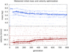 |
Fig. 1 Example of the initial mass and velocity evolution of the meteoroid for the best solution of the EN020615. The solid line shows the starting values that were found by the procedure detailed in the text: an initial mass of 5.0 kg, and an initial velocity of 16.18 km s−1. The width of the searched interval of values was set to ±1.5 kg for the mass and ±0.1 km s−1 for the velocity. |
3.8 Initial mass and velocity
To successfully model the fireball, we first need to estimate the initial mass and velocity of the meteoroid. The initial velocity is calculated by fitting the linear part of the dynamics curve by a straight line (length versus time; the velocity is the slope). This value is usually precise enough, but we still allowed for some small changes in the modeling process. We let the algorithm randomly choose the initial velocity from the interval around the initial value and form the sample solution with this value. The size of the interval at the beginning of the process was 0.2 km s−1 and was decreased to 0.05–0.1 km s−1 as the best solution is approached. The initial height is optimized during modeling as well to obtain a consistent solution of the meteoroid dynamics.
The initial guess of the mass was first calculated by integrating the radiometric light curve (or a regular light curve), which yielded the radiated energy. Then we set the radiated energy equal to the kinetic energy of the body, multiplied by the assumed luminous efficiency (τ). We used the function of Borovička et al. (2020), which depends on the velocity (already calculated) and the mass, which we were about to calculate. Therefore, we calculated the mass iteratively, that is, we calculated the mass with an initial guess of τ, and we updated the mass and τ until the mass converged to some value that no longer changed (usually only a few iterations). By this approach, we usually obtained a lower bound of the mass because the smaller fragments have lower τ and τ also decreases with decreasing velocity. A more precise value has to be calculated in the optimization process in the same way as the velocity. The size of the interval was initially set to 0.5 of the mass value and was decreased as appropriate. An example of the initial velocity and mass convergence in the optimization process is given in Fig. 1.
3.9 Search for fragmentations
The current version of the FirMpik program is not able to find fragmentation times in the radiometric curve data. Therefore, we have to search for them manually. We marked the approximate fragmentation times, and then we increased its precision through an automatic process.
The gross fragmentation is usually visible in the curve as a fast or immediate and obvious brightening, followed by a more gradual dimming of the fireball. They are modeled as a sudden breakup of a parent fragment with a dust release. On the other hand, continuous fragmentations are more subtle, and some experience is required to successfully find it. We modeled continuous fragmentations as an erosion of dust particles from a single fragment. More than one fragment occasionally starts to erode at a given fragmentation time, with a different erosion coefficient and size distribution of the released particles. Through this, we can fit some more complicated shapes of the radiometric data (e.g., different slopes).
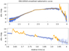 |
Fig. 2 Smoothed radiometric curve of the EN110918 shown by orange dots with error impulses, compared with the original, labeled by blue pluses with error impulses. The upper panel shows the whole radiometric curve, and the lower panel shows the end of it in greater detail. The flares are copied from the original curve, and the other parts are filtered using the median running box. |
3.10 Smoothing of the radiometric curve
Radiometric curves contain very fine details of the fireball brightness because their sampling rate is 5000 Hz. They contain semi-harmonic brightness changes whose origin is still debated (e.g., Beech & Brown 2000; Babadzhanov & Konovalova 2004; Spurný & Ceplecha 2008; Spurný et al. 2012). Our current model, however, does not contain a description of these rapid changes, and therefore, we needed to remove the changes from the radiometric curve for a successful modeling. On the other hand, we need to preserve all the details of the gross fragmentations and general trends that we model with the FirMpik program. We therefore manually separated the radiometric curve into two parts, one part that contained the data points of the flares and their close vicinity, and the other part contained the outside parts. The latter curve was then automatically smoothed by the running-box median filter with an appropriate box width. This procedure reliably removes the rapid brightness variations, but preserves the general trends in fireball brightness. The parts of the curve that contain the gross fragmentations remain unchanged. An example of a smoothed radiometric curve is shown in Fig. 2.
Moreover, for a successful automatic modeling, it is not practical to work with such a high sampling rate of the radiometric curve, unless we wish to model its very fine structure. Therefore, we decided to automatically dilute the part of the radiometric curve that lies outside the gross fragmentations. Another reason is that in modeling, we wish to have a comparable number of data points for each data set, that is, for the radiometric curve and the light curve, and for the dynamics as well. It helps the algorithm to fit the data with a similar priority.
For each fireball, we needed to test the appropriate box width for the running-box median filter. Therefore, we calculated the smoothed curve with different box widths and then selected the width that captured all the main features of the original radiometric curve.
3.11 Dataset weights
The first attempts to automatically model the fireball data were not very successful. For instance, we obtained a perfect fit for the dynamics of the fireball and a much poorer fit for the radiometric curve and light curve. This was probably caused by an unknown conversion between brightness and distance contributions to the χ2 sum (the inverse of which is our fitness), or simply put, by a magnitude-kilometer conversion factor. Moreover, our datasets usually have a different number of data points, and those data have also different uncertainties. Therefore, we experimentally set different weights to each dataset in the χ2 value calculation to show the algorithm what to focus on when individual solutions were evaluated. After some experimenting with the specific weight values, we were able to obtain a more reasonable fit for both datasets. The specific setting of the weight is still rather empirical, and it is a source of uncertainty when we start calculating the new fireball. The current approach is to run several individual calculations with a wide range of weights, to choose those that are more viable, and to gradually narrow down the span of the weights. The current construction of the optimization process does not allow setting the weights as a free parameter.
3.12 Largest impact on the χ2 sum
To keep the number of free parameters low, we tested which of them were the most important and which were less important. We fixed all the parameters except for one, and inspected the change in the χ2 sum. Thus we found that the number of fragments had largest impact on the χ2 value, especially the fragments that were released from the meteoroid in the first fragmentation. The second most important parameter was an erosion of some of the released fragments. The erosion controls the overall shape and slope of the total brightness curve in the model. The third most important group of parameters were the fragment masses and the dust mass. The dust mass distribution limits were less important because they mainly affect the shape of the flares, but the flares are usually short and therefore have little effect on the total χ2 sum.
3.13 RLC weights
To further emphasize the importance of gross and continuous fragmentations within the radiometric curve, we decided to set higher weights for the vicinity of the fragmentation times in the χ2 sum calculation. Using this approach, we can tell the algorithm which parts on the radiometric curve have to be fit more precisely and where the fit can be looser.
3.14 Modeling outputs
The fireball modeling yields several important parameters describing the fragmentation of the meteoroid in the atmosphere. These are the number of fragments in each fragmentation time, their respective masses, whether or not the fragment erodes, its erosion coefficient, and the mass limits of the eroded dust grains. Moreover, we determine the amount of dust released in gross fragmentations and schematically determine the mass distribution of the dust. The model optimizes the initial velocity and mass of the meteoroid, so that we obtain more precise values than we can calculate from the dynamics and radiometric curve alone. The program can also resolve whether some meteorites may be found on the ground and their number and respective masses.
From the model, we deduced the height of the fragmentation for each fragmentation time. Based on this, we can calculate the atmospheric density at that height. Using the measured velocity at the same time, we calculated the dynamic pressure (p = ρυ2) acting on the front part of the meteoroid. This is a proxy for a meteoroid shear strength (Robertson & Mathias 2017), and it is a very important mechanical parameter of the meteoroid material. In this way, we can compare different meteoroid materials and in turn obtain other constraints on the properties of its parent body. More clues about the origin of the meteoroid can be deduced from the whole fragmentation process (how it breaks up, whether it erodes or not, etc.). The data on fragment masses and their strength approximation (just before their fragmentation) can then be plotted in log-log plane, as shown for the test fireballs presented in this paper in Sect. 4. In this way, we can also compare different solutions of a single meteoroid fragmentation.
Because of the extensive use of pseudo-random numbers, the algorithm is inherently stochastic. To obtain a reliable fit of the fireball data, we need to run the calculation several times to some tens of times and then process the results statistically. The number of runs depends on the number of data at hand, on their complexity (e.g., the number of fragmentation times and other features of radiometric data), and thus mainly on the number of free parameters we need to find. The number of free parameters is proportional to the number of fragments that are produced during meteoroid fragmentation,
 (7)
(7)
For each run, we typically obtained several hundred best-fitting solutions with almost the same χ2 value that are nearly identical. In two different runs, the fits were of comparable quality, but the details of the fragmentation of the meteoroid can differ. From the set of the best solutions, we can estimate the uncertainties, that is, we can calculate the most probable number of fragments in each fragmentation time, the masses of individual fragments, and so on.
3.15 Uncertainties
The initial idea of calculating the uncertainties of (some of) the free model parameters was to calculate the χ2 value threshold, which is an equivalent of a one sigma confidence interval for a single measured value by a standard statistical theory. However, this was not possible in our case mainly because the modeling problem is not linear in those parameters (Bevington & Robinson 2003; Andrae 2010). As noted above, the reduced χ2 value therefore does not have the usual statistical meaning and cannot be used to calculate the probability of finding the optimized parameter in a certain interval around the value found by the optimization.
To find some equivalent of the uncertainties of the quantities obtained in the simulations, we decided to use the approach of Gibson & Charbonneau (1998). The uncertainties of the initial velocity and mass of the meteoroid were estimated based on the set of (some hundred) acceptable solutions with a χ2 value lower than some chosen threshold value. In our case, it was arbitrarily set to 1.1 of the χ2 value of the respective acceptable solution (each acceptable solution had a different minimum χ2 value). In this way, we constructed histograms of initial masses and velocities that were indicative of a confidence interval. It would probably require many more successfully converged simulations for a single fireball to numerically describe the underlying (complicated) distribution of the optimized quantities and to derive a statistically meaningful confidence interval for those quantities as an interval between, for instance, the 5th and 95th percentile. However, this is too expensive computationally.
Another possibility is to calculate the uncertainties using the Monte Carlo method (Press et al. 1992). This requires using the current datasets with their intrinsic uncertainties, to prepare many hundreds to thousands of synthetic datasets within these data uncertainty intervals, and then optimizing these datasets only to obtain a sampling of the free model parameters, which enables us to derive their uncertainties. This is perfectly viable when data with a moderately complicated model need to be fit that takes seconds to minutes to calculate. An order-of-magnitude estimate of the computation time for our problem, however, gives some thousands to tens of thousands of hours of computation time, which is an unreasonably long time. Therefore, we decided to present the uncertainties of some of the free model parameters only in the form of plots showing the best solutions without a more rigorous quantification (see Sects. 4.2 and 4.3).
4 Results
4.1 Manual modeling comparison
The correct function of the algorithm was tested by a blind test that was constructed in the following way. One of us (JB) chose five previously modeled fireballs with abundant data taken with the EN that were described by Borovička et al. (2020). The other author (TH) then prepared the data for the automatic modeling and ran a different number of simulations for each fireball. The number of simulations spanned from 10 to 70. One reason for the high number of simulations for each fireball is the stochasticity of the algorithm, which was initialized randomly, and all the genetic operations are also probabilistic and were calculated with pseudo-random numbers.
The simulations were evaluated, and the best solutions were chosen based on the reduced χ2 value and the overall look of the fits of the radiometric curve, photometric light curve, and dynamic data. The best solutions were then compared to the manual solutions of Borovička et al. (2020). In the following, we describe the solutions for the five fireballs in detail. The figures for four fireballs are presented in Appendix A. The name of a fireball observed by the EN contains the EN prefix, followed by the date and time (UT) of the fireball observation start in the format ENddmmyy_hhmmss. We give the full name for each fireball first, but then we use a short form of ENddmmyy to refer to it.
EN260815_233145
This fireball was caused by a 6.5 kg meteoroid traveling at 19.3 km. s−1. First, a very gradual brightening of the fireball was observed, while at the same time, there were very fast semi-periodic variations in the radiometric curve. In the second half of the curve, three very bright flares were observed (the first flare was the brightest at −11.7 mag), and one not very conspicuous flare occurred at the end. These flares served as unequivocal fragmentation times in the modeling.
This fireball was the first that we attempted to model with the FirMpik program. It also served as a model case for developing the optimization function and for thorough testing of the code that preceded the production runs of the following fireballs. Because the fragmentation points are more or less obvious in the radiometric curve, the modeling was relatively easy. The hardest part in modeling this and also other fireballs is to reconcile the radiometric curve with the dynamic data at the very end of observations. This is one of the reasons we had to calculate several (tens of) runs.
The automatic solution in Fig. 3 is very similar to the manual solution in Fig. 4, although the flares are not fit with the same precision and the model is slightly brighter at the end of observations. Residuals of dynamics fit are shown in Figs. 5 and 6 for the automatic and manual solutions, respectively.
As we mentioned above, the dynamic data only refer to the foremost fragment, but it is a very important piece of information. While the radiometric curve alone can be fit by a large number of fragment combinations, the dynamic data constrain the plausible combinations because they sensibly check the size of the foremost fragment (smaller fragments decelerate more than larger ones). It is also an independent check on whether we correctly found the fragmentation times.
We expect the points in the O–C plot to be randomly and symmetrically distributed around the blue gravity expectation curve (because gravity accelerates the meteoroid and its fragments). There should be no trends or periodic behavior, and a reasonable dispersion of the points is on the order of a hundred meters for high-quality data.
The two solutions are also compared graphically in Fig. 7, where the disruption cascade is depicted schematically. The cascades differ, but the eroding versus ablating mass ratio is similar at any instant displayed in the plot in both solutions. The first model predicts a mass that is twice higher in meteorites than the second model (0.24 kg vs. 0.12 kg), which corresponds to the higher modeled brightness at the end.
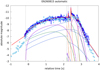 |
Fig. 3 Automatic solution of the EN260815 fragmentation compared to the observed radiometric curve (dark blue pluses) and a photometric light curve (sky blue disks). The total model brightness is shown as a solid red line, the brightness of regular fragments is shown as blue curves, green curves signify eroding fragments, violet lines indicate dust particles released from these fragments, and orange curves denote regular dust released in gross fragmentations. Fragmentation times are shown with vertical dashed lines. |
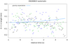 |
Fig. 5 Residuals of length for an automatic solution of the EN260815. Different colors indicate the stations of the EN that were used to calculate the model. The solid blue line predicts the acceleration of the meteoroid by gravity. |
EN110918_214648
This relatively bright fireball was caused by a 6.5 kg meteoroid traveling at 23.5 km. s−1. The radiometric curve begins with a gradual brightening that takes almost 1.25 s and is followed by a plateau. At t = 2.8 s, some brighter semiperiodic brightness variations appear in the curve. These are followed by a series of nine flares that signify important breakups of the meteoroid. Four of them are very bright (the brightest reached −14.25 mag). In the end, the overall brightness of the fireball decreases very rapidly.
This fireball was among the most difficult to model. It was straightforward to find the fragmentation times because they are indicated by very bright and short flares in the radiometric curve. In the first step, we used a moderate time resolution of 0.01 s, and after several attempts, we successfully modeled the fireball (Fig. A.1). At this time resolution, however, some of the bright flares (gross fragmentations) were heavily smeared. Therefore, we increased the time resolution to 0.005 s, and after varying the weights and also fixing the initial velocity and initial mass of the meteoroid found in the previous modeling, we were able to find a good solution with this higher time resolution as well (Fig. A.2). The manual solution fits the radiometric curve even better with more details (Fig. A.3). The length residuals shown in Figs. A.4 and A.5 are almost the same. In this case, we did not use photometric data to construct the model, and therefore they are not plotted in the figures.
EN240217_190640
This fireball was caused by a meteoroid of 2.5 kg traveling at 17.8 km. s−1 with extremely high semiperiodic variations in brightness in the radiometric curve. On the other hand, we did not observe any obvious gross fragmentations that usually manifest themselves in the curve by a sudden brightening on the order of some tenths to several magnitudes. Therefore, the fragmentation times used in the modeling are less certain, and they were needed to sensibly fit the overall shape of the radiometric and photometric data as well as the dynamics of the meteoroid. The automatic solution (Fig. A.6) is very good and comparable to the manual solution (Fig. A.7), except for one detail: In the manual solution, Borovička et al. (2020) attempted to model some of the brightenings at the beginning as gross fragmentations. However, the overall mass loss in these fragmentations was negligible, and they had little effect on the latter parts of the light curve and on the dynamics. The residuals of the dynamic fit were somewhat better for the automatic solution, especially in the time interval 3–4 s (Figs. A.8 and A.9).
EN020615_215119
This fireball was caused by a 5 kg meteoroid traveling at 16.2 km. s−1. The brightness variations of the fireball are present in the radiometric curve from the very beginning. The initial increase in brightness is very fast and progressive, and at time 2 s, the fireball reaches maximum brightness, experiencing large semiperiodic variations in brightness at the same time. A brightness plateau follows, and after t = 3 s, the brightness starts to drop gradually. As usual, there is a series of flares in the radiometric curve: We observe five of them, while the overall brightness of the fireball decreases gradually. The automatic (Fig. A.10) and manual (Fig. A.11) solutions are similar, except for the beginning, where the first fragmentation time was chosen differently and the manual solution used only one fragmentation. This resulted in a poorer fit. The length residuals have a similar dispersion in both cases (Figs. A.12 and A.13), but their distribution at the beginning in the manual solution is more even.
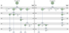 |
Fig. 7 Comparison of the automatic (left panel) and manual (right panel) solution for EN260815. The solid disks are regular ablating fragments, and the spotted disks with a dotted border are eroding fragments. The time runs from top to bottom, numbers in the disk center are fragment names, the number to the right of the disk is the initial mass of the fragment in kg, and the number at the bottom of the disk is the fragment erosion coefficient η in kg MJ−1. The final mass (also in kg) of the fragment before its fragmentation is shown as blue rectangles. Slight differences in dynamic pressures are caused by two different models of atmosphere in these two solutions. |
EN180118_182623
The initial mass of the meteoroid causing this fireball was slightly lower than 3 kg, and it traveled at 20.0 km. s−1. The first half of the radiometric curve is very smooth, without any significant semiperiodic variations in brightness, while the second half of the curve is quite the opposite. At the time 3.0 s, there is a drop in brightness that cannot be explained by the current model, and we therefore decided to ignore it in the modeling process. The model only roughly fits the brightness in that place. Then the fast variations in brightness appear in the curve, and they completely disappear at time 3.85 s, reappearing again at 4.1 s. No flares are apparent in the radiometric curve, which complicates the modeling. We decided to estimate the fragmentation times based on changes in brightness trends in the radiometric curve. This led to a less satisfactory model fit than in the previous cases. The end of the radiometric curve in particular is poorly fit (Fig. A.14). The manual solution is better (Fig. A.15), mainly because of the better fit of the aforementioned brightness drop and also because of the more extensive use of gross fragmentations between ~3.8–4.6 s, which allowed the substantial mass loss of the meteoroid and in turn a better fit. The automatic algorithm is not able to use this process when it is not clearly present in the data, because it optimizes the χ2 sum with respect to the median radiometric curve, and these departures would cause a higher χ2 sum and therefore lower fitness value. In the future, we wish to address this problem with a more versatile fitness value or a different χ2 calculation. The length residuals are then shown in Figs. A.16 and A.17. They support the quality comparison of the two solutions. Both of them have a less satisfactory fit around the time 4 s.
4.2 Initial mass and velocity uncertainties
The uncertainties of the initial mass and velocity of the meteoroid are presented in Figs. 8 and 9. They show the spread of the respective values for the 11 best solutions of the EN020615 fireball found by the FirMpik program. Each histogram shows with a specific color the distribution of initial mass (velocity) of the meteoroid for a single solution and its close vicinity as measured by the χ2 value. The width of the histogram columns reflects the spread of the mass (velocity) values for each best solution (the number of histogram columns was fixed). The shape of individual histograms is caused by the nature of the GA approach to finding a solution. The spread of the initial mass and velocity values and the overall shape of all histograms in Figs. 8 and 9 suggests a complicated distribution of the uncertainties. The details of this procedure were described above in Sect. 3.15. For other fireballs, the uncertainty distribution looks similar. For comparison, the manual solution of the EN020615 gave an initial mass of the meteoroid of 5.0 kg and an initial velocity of 16.28 km. s−1.
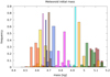 |
Fig. 8 Spread of the initial mass for EN020615. The spread displays its uncertainty. The plot shows the 11 best solutions and their vicinity with bars of different colors. |
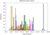 |
Fig. 9 Spread of the initial velocity for EN020615. The spread displays its uncertainty. The same color as in Fig. 8 marks the same solution. |
4.3 Pressure-mass plot
The results of the automatic and manual approach can be compared in the dynamic pressure-fragment mass space. It shows the masses of fragments released from the meteoroid and later from its fragments, and it also shows whether the same fragmentation times were found by both methods, which then leads to the same values of the dynamic pressure. Figure 10 shows that both methods give similar results (open symbols versus solid symbols of the same shape and color). Some differences are also clear: The automatic method produces some very low fragment masses, which are allowed by the wider span of fragment masses to choose from. The main cause for this behavior may be the process of the solution evolution itself. For example, the algorithm initially chooses the greater mass of a specific fragment, but it later finds that this fragment mass should be negligible or zero, which is currently not allowed in the optimization function. Therefore, the mass of this fragment evolves to very low values until it has little effect on the overall solution (mainly total brightness). In a future version of the program, we wish to resolve this issue.
This plot can be used to estimate the uncertainties of the fragment masses and the dynamic pressure at which the meteoroid and its descendant fragments break. A very simplistic solution is to filter all important fragments (that contribute to the model light curve) and then calculate the arithmetic mean (or median) and a statistical error of the mean of their respective masses and dynamic pressures.
5 Discussion
After modeling the five fireballs presented in this paper, we describe a few critical points of the modeling. The first point is the unequivocal determination of fragmentation times. As we already mentioned, gross fragmentations are usually found easily because they appear as bright flares in the radiometric curve. This was not always the case, however, and then it was more problematic to successfully model the fireball fragmentation. The fragmentations that produce eroding fragment(s) are even more difficult to find, and it is also not possible to set it as precisely as the gross fragmentation. It is usually marked by a change in the overall slope of the radiometric curve, but finding such a point requires some modeling experience and experimenting. This also propagates to the results of the modeling process: it affects the derived mechanical strength of the meteoroid or its fragments.
The second critical point is finding the proper weights for individual datasets (radiometric curve, light curve, and dynamic data) when calculating the χ2 sum. This seems to have a substantial effect on finding an acceptable solution to fireball fragmentation. We described the probable physical interpretation of these weights in detail in Sect. 3.11. Nevertheless, it is one of the critical values that we need to experimentally assign to each run from a plausible range, and we have still little understanding of what the value should be beforehand.
Furthermore, the price for a better fit is usually the production of more fragments from the meteoroid and the higher complexity of the model. This should mostly be avoided because it is questionable whether the data support such a complex model. We recall that the number of free parameters grows with the number of fragments. Moreover, we note that the automatic model sometimes contains some very little fragments that do not manifest themselves in the available data, they are rather numerical artifacts. Therefore, we prefer the models with a lower number of fragments involved, as in the manual solution, and we follow the principle of Occam’s razor. We note that this preference may lead to biased solutions. In the future version of the program, we will focus more on this problem, and we consider that the total number of fragments may be one of the criteria for an acceptable solution that can be forced already in the optimization process. It should not be difficult to model any data with a huge number of free parameters, but it is hardly justifiable.
We do not claim that the current approach can find a unique solution to the problem. However, it is mostly able to find a solution that is consistent with all the available data we have about meteoroid atmospheric fragmentation. We note that as with any numerical model, our model is also simplified and cannot capture all the fine details of the process. For instance, there could be smaller fragments that do not substantially contribute to the overall brightness of the fireball, and they do not have an impact on dynamics. In this sense, there could be many equally good solutions with a different number of fragments for a single fireball, and the solution we presented is only one representative solution of this set.
As noted above, we usually employed a computation cluster comprising a few dozen nodes with 48 threads (24 physical cores) each. The computation of a single model on a single node took tens of hours to a few days, depending on the complexity of optimized data. We will consider a few ways to improve the speed of the computation in the future.
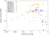 |
Fig. 10 Comparison of automatic (open symbols) and manual (solid symbols) meteoroid fragmentation modeling in dynamic pressure-fragment mass space. The dynamic pressure is the atmospheric pressure exerted on a meteoroid or a fragment derived from it just before another fragmentation. Results of 7–11 automatic solutions with an acceptable quality are shown for each fireball, except for the case of EN180118, for which only two solutions of poor quality are shown. |
6 Conclusions
In this paper, we presented the semi-automatic program called FirMpik, which can find quality solutions for fireball fragmentation in the atmosphere consistent with the radiometric and photometric data as well as the dynamics of the meteoroid. When compared to the manual approach, the program can find a solution of similar quality and sometimes a solution that is formally slightly better. However, we demonstrated on some fireballs that it cannot find a substantially better solutions. It also did not find solutions that would fit data similarly, but would be markedly different. The meteoroid fragments into a similar number of fragments that have roughly the same mass; where there is an eroding fragment in the manual solution, the automatic one features one (or a few) eroding fragments as well. This was shown in Sect. 4.
These automatic solutions consistently map in the same region of the dynamic pressure-fragment mass space as the manual solutions. The only difference is that they often comprise a greater total number of fragments than the manual solutions. In the current version of the program, the number of fragments for each fragmentation time is selected randomly from a hard-wired span of values, but more constraints can be placed on this process in the future version of the program.
The uncertainties of the calculated quantities (dynamic pressure, fragment masses, initial meteoroid velocity, and mass) were estimated from the spread of the values in different solutions of similar quality. This was not possible before in the manual procedure, where only one solution was found for each fireball. However, we were not able to find a more rigorous and computationally viable way to calculate uncertainties.
Currently, we have to find the fragmentation times in the data manually and then increase their precision with an automatic procedure. Then, we estimate a plausible range of weights of available datasets and run several (tens of) simulations to find the most plausible value. At the same time, we employ a wide range of the initial meteoroid mass and velocity values and a wider range of fragment numbers in each fragmentation time. Later, when we find more viable types of solutions, we narrow these ranges down, which enables a faster search of the parametric space, and we find a global optimum of the problem more likely.
We usually need to run a few to several tens of runs before we find a quality fit to the fireball data. This is necessary because of the inherent stochasticity of the optimization process. During the computation, the algorithm extensively uses pseudo-random numbers, and it is also randomly initialized. Still, the algorithm converges to similar solutions that have a comparable χ2 value, as we expected. The nature of the GA also promotes a thorough search of the parametric space, because several tens to hundreds of individuals are dispersed and search independently for the solution. Moreover, the data we have about meteoroid fragmentation are complementary and further constrain the potential solution. Therefore, the algorithm is in most cases capable of finding a global optimum that fits all the available data. With all the model simplifications, this solution consistently describes the fireball fragmentation in the atmosphere.
In the future, we would like to improve finding the fragmentation times, make it more robust, and make it part of the optimization process. A more in-depth understanding of the dataset weights is our next goal as well. Last, we would like to place more constraints on the model to be more confident about the uniqueness of the solution by employing more data for this procedure, for instance, data on individual fragments observed for some fireballs with narrow-field-of-view cameras.
Acknowledgements
We are grateful to Donovan Mathias for a very careful and constructive review that helped us substantially improve the presentation of our research. This research was supported by grant no. 19-26232X from the Czech Science Foundation. The computations were performed on the OASA and VIRGO clusters of the Astronomical Institute of the Czech Academy of Sciences. This research has made use of NASA’s Astrophysics Data System.
Appendix A Additional figures
In this appendix, we present additional figures that compare the results of the automatic and the manual modeling of the other four bolides. They are described in detail in Sect. 4.
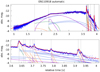 |
Fig. A.1 Automatic solution for EN 110918 in a lower time resolution of tres = 0.01 s. The upper panel shows the whole radiometric curve, and the lower panel shows the end of it in greater detail. Some of the details at the end of the radiometric curve are not present in the model. Labels are the same as in Fig. 3. |
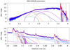 |
Fig. A.2 Best obtained automatic solution to EN110918 in higher time resolution of tres = 0.005 s. Labels are the same as in Fig. 3. |
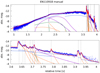 |
Fig. A.3 Manual solution for EN110918 with the same time resolution as the best automatic solution. Labels are the same as in Fig. 3. |
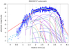 |
Fig. A.6 Automatic solution of EN240217 compared to radiometric and light-curve data. Labels are the same as in Fig. 3. |
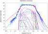 |
Fig. A.10 Automatic solution for EN020615 compared to radiometric and light-curve data. Labels are the same as in Fig. 3. |
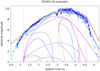 |
Fig. A.14 Automatic solution for EN180118 compared to radiometric and light-curve data. Labels are the same as in Fig. 3. |
References
- Ahrens, T. J., Takata, T., O’Keefe, J. D., & Orton, G. S. 1994, Geophys. Res. Lett., 21, 1087 [NASA ADS] [CrossRef] [Google Scholar]
- Akimov, V. A., Glazachev, D. O., Emel’yanenko, V. V., et al. 2015, in Asteroids and Comets Hazard (Moscow: Strategy of Counteraction), 272 [Google Scholar]
- Anderson, E., Bai, Z., Bischof, C., et al. 1999, LAPACK Users’ Guide, 3rd edn. (Philadelphia, PA: Society for Industrial and Applied Mathematics) [CrossRef] [Google Scholar]
- Andrae, R. 2010, ArXiv e-prints [arXiv:1009.2755] [Google Scholar]
- Babadzhanov, P. B., & Konovalova, N. A. 2004, A&A, 428, 241 [NASA ADS] [CrossRef] [EDP Sciences] [Google Scholar]
- Baldwin, B., & Sheaffer, Y. 1971, J. Geophys. Res., 76, 4653 [NASA ADS] [CrossRef] [Google Scholar]
- Beech, M., & Brown, P. 2000, Planet. Space Sci., 48, 925 [NASA ADS] [CrossRef] [Google Scholar]
- Bevington, P. R., & Robinson, D. K. 2003, Data Reduction and Error Analysis for the Physical Sciences, 3rd edn. (New York, NY: McGraw-Hill) [Google Scholar]
- Borovička, J., Spurný, P., & Koten, P. 2007, A&A, 473, 661 [NASA ADS] [CrossRef] [EDP Sciences] [Google Scholar]
- Borovička, J., Spurný, P., Brown, P., et al. 2013a, Nature, 503, 235 [NASA ADS] [Google Scholar]
- Borovička, J., Tóth, J., Igaz, A., et al. 2013b, Meteorit. Planet. Sci., 48, 1757 [Google Scholar]
- Borovička, J., Spurný, P., & Shrbený, L. 2020, AJ, 160, 42 [CrossRef] [Google Scholar]
- Boslough, M. B., Crawford, D. A., Robinson, A. C., & Trucano, T. G. 1994, Geophys. Res. Lett., 21, 1555 [NASA ADS] [CrossRef] [Google Scholar]
- Brown, P. G., Assink, J. D., Astiz, L., et al. 2013, Nature, 503, 238 [NASA ADS] [Google Scholar]
- Ceplecha, Z., Borovička, J., Elford, W. G., et al. 1998, Space Sci. Rev., 84, 327 [NASA ADS] [CrossRef] [Google Scholar]
- Charbonneau, P. 1995, ApJS, 101, 309 [Google Scholar]
- Charbonneau, P. 2002a, NCAR Technical Note 450+IA [Google Scholar]
- Charbonneau, P. 2002b, NCAR Technical Note 451+STR [Google Scholar]
- Charbonneau, P., & Knapp, B. 1995, NCAR Technical Note 418+IA [Google Scholar]
- Darwin, C. 1859, On the Origin of Species by Means of Natural Selection, or the Preservation of Favoured Races in the Struggle for Life (London: Murray) [Google Scholar]
- Eiben, A. E., & Smith, J. E. 2015, Introduction to Evolutionary Computing, 2nd edn. (Berlin: Springer Publishing Company, Incorporated) [CrossRef] [Google Scholar]
- Geist, A., Beguelin, A., Dongarra, J., et al. 1994, PVM: A Users’ Guide and Tutorial for Network Parallel Computing (Cambridge: The MIT Press) [CrossRef] [Google Scholar]
- Gibson, S. E., & Charbonneau, P. 1998, J. Geophys. Res., 103, 14511 [NASA ADS] [CrossRef] [Google Scholar]
- Hills, J. G., & Goda, M. P. 1993, AJ, 105, 1114 [NASA ADS] [CrossRef] [Google Scholar]
- Kartashova, A. P., Popova, O. P., Glazachev, D. O., et al. 2018, Planet. Space Sci., 160, 107 [NASA ADS] [CrossRef] [Google Scholar]
- Metcalfe, T. S. 2001, PhD thesis, University of Texas, Austin, Texas, USA [Google Scholar]
- Metcalfe, T. S., & Charbonneau, P. 2003, J. Comput. Phys., 185, 176 [NASA ADS] [CrossRef] [Google Scholar]
- Öpik, E. J. 1955, Irish Astron. J., 3, 165 [Google Scholar]
- Picone, J. M., Hedin, A. E., Drob, D. P., & Aikin, A. C. 2002, J. Geophys. Res. Space Phys., 107, 1468 [Google Scholar]
- Popova, O. P., Jenniskens, P., Emel’yanenko, V., et al. 2013, Science, 342, 1069 [NASA ADS] [CrossRef] [Google Scholar]
- Popova, O., Borovička, J., & Campbell-Brown, M. D. 2019, in Meteoroids: Sources of Meteors on Earth and Beyond, eds. G. O. Ryabova, D. J. Asher, & M.J. Campbell-Brown (Cambridge: Cambridge University Press), 9 [Google Scholar]
- Press, W. H., Teukolsky, S. A., Vetterling, W. T., & Flannery, B. P. 1992, Numerical Recipes in FORTRAN 77: the Art of Scientific Computing (USA: Cambridge University Press) [Google Scholar]
- Robertson, D. K., & Mathias, D. L. 2017, J. Geophys. Res. Planets, 122, 599 [NASA ADS] [CrossRef] [Google Scholar]
- Spurný, P., & Ceplecha, Z. 2008, A&A, 489, 449 [NASA ADS] [CrossRef] [EDP Sciences] [Google Scholar]
- Spurný, P., Borovička, J., & Shrbený, L. 2007, IAU Symp., 236, 121 [Google Scholar]
- Spurný, P., Bland, P. A., Shrbený, L., et al. 2012, Meteorit. Planet. Sci., 47, 163 [CrossRef] [Google Scholar]
- Spurný, P., Borovička, J., Baumgarten, G., et al. 2017, Planet. Space Sci., 143, 192 [Google Scholar]
- Svetsov, V. V., Nemtchinov, I. V., & Teterev, A. V. 1995, Icarus, 116, 131 [NASA ADS] [CrossRef] [Google Scholar]
- Tárano, A. M. 2020, PhD thesis, Stanford University, Stanford, California, USA [Google Scholar]
- Tárano, A. M., Wheeler, L. F., Close, S., & Mathias, D. L. 2019, Icarus, 329, 270 [CrossRef] [Google Scholar]
- Wheeler, L. F., Register, P. J., & Mathias, D. L. 2017, Icarus, 295, 149 [NASA ADS] [CrossRef] [Google Scholar]
- Wheeler, L. F., Mathias, D. L., Stokan, E., & Brown, P. G. 2018, Icarus, 315, 79 [NASA ADS] [CrossRef] [Google Scholar]
The source code for PIKAIA and some of the cited references can be found at https://www.hao.ucar.edu/modeling/pikaia/pikaia.php.
All Figures
|
Fig. 1 Example of the initial mass and velocity evolution of the meteoroid for the best solution of the EN020615. The solid line shows the starting values that were found by the procedure detailed in the text: an initial mass of 5.0 kg, and an initial velocity of 16.18 km s−1. The width of the searched interval of values was set to ±1.5 kg for the mass and ±0.1 km s−1 for the velocity. |
| In the text | |
|
Fig. 2 Smoothed radiometric curve of the EN110918 shown by orange dots with error impulses, compared with the original, labeled by blue pluses with error impulses. The upper panel shows the whole radiometric curve, and the lower panel shows the end of it in greater detail. The flares are copied from the original curve, and the other parts are filtered using the median running box. |
| In the text | |
|
Fig. 3 Automatic solution of the EN260815 fragmentation compared to the observed radiometric curve (dark blue pluses) and a photometric light curve (sky blue disks). The total model brightness is shown as a solid red line, the brightness of regular fragments is shown as blue curves, green curves signify eroding fragments, violet lines indicate dust particles released from these fragments, and orange curves denote regular dust released in gross fragmentations. Fragmentation times are shown with vertical dashed lines. |
| In the text | |
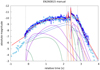 |
Fig. 4 Manual solution of EN260815. Labels are the same as in Fig. 3. |
| In the text | |
|
Fig. 5 Residuals of length for an automatic solution of the EN260815. Different colors indicate the stations of the EN that were used to calculate the model. The solid blue line predicts the acceleration of the meteoroid by gravity. |
| In the text | |
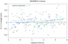 |
Fig. 6 Residuals of the length for a manual solution for EN260815. Labels are the same as in Fig. 5. |
| In the text | |
|
Fig. 7 Comparison of the automatic (left panel) and manual (right panel) solution for EN260815. The solid disks are regular ablating fragments, and the spotted disks with a dotted border are eroding fragments. The time runs from top to bottom, numbers in the disk center are fragment names, the number to the right of the disk is the initial mass of the fragment in kg, and the number at the bottom of the disk is the fragment erosion coefficient η in kg MJ−1. The final mass (also in kg) of the fragment before its fragmentation is shown as blue rectangles. Slight differences in dynamic pressures are caused by two different models of atmosphere in these two solutions. |
| In the text | |
|
Fig. 8 Spread of the initial mass for EN020615. The spread displays its uncertainty. The plot shows the 11 best solutions and their vicinity with bars of different colors. |
| In the text | |
|
Fig. 9 Spread of the initial velocity for EN020615. The spread displays its uncertainty. The same color as in Fig. 8 marks the same solution. |
| In the text | |
|
Fig. 10 Comparison of automatic (open symbols) and manual (solid symbols) meteoroid fragmentation modeling in dynamic pressure-fragment mass space. The dynamic pressure is the atmospheric pressure exerted on a meteoroid or a fragment derived from it just before another fragmentation. Results of 7–11 automatic solutions with an acceptable quality are shown for each fireball, except for the case of EN180118, for which only two solutions of poor quality are shown. |
| In the text | |
|
Fig. A.1 Automatic solution for EN 110918 in a lower time resolution of tres = 0.01 s. The upper panel shows the whole radiometric curve, and the lower panel shows the end of it in greater detail. Some of the details at the end of the radiometric curve are not present in the model. Labels are the same as in Fig. 3. |
| In the text | |
|
Fig. A.2 Best obtained automatic solution to EN110918 in higher time resolution of tres = 0.005 s. Labels are the same as in Fig. 3. |
| In the text | |
|
Fig. A.3 Manual solution for EN110918 with the same time resolution as the best automatic solution. Labels are the same as in Fig. 3. |
| In the text | |
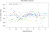 |
Fig. A.4 Length residuals of the automatic model of EN110918. Labels are the same as in Fig. 5. |
| In the text | |
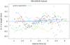 |
Fig. A.5 Length residuals of the manual model of EN110918. Labels are the same as in Fig. 5. |
| In the text | |
|
Fig. A.6 Automatic solution of EN240217 compared to radiometric and light-curve data. Labels are the same as in Fig. 3. |
| In the text | |
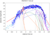 |
Fig. A.7 Manual solution for EN240217. Labels are the same as in Fig. 3. |
| In the text | |
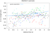 |
Fig. A.8 Length residuals of the automatic model for EN240217. Labels are the same as in Fig. 5. |
| In the text | |
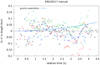 |
Fig. A.9 Length residuals of the manual model for EN240217. Labels are the same as in Fig. 5. |
| In the text | |
|
Fig. A.10 Automatic solution for EN020615 compared to radiometric and light-curve data. Labels are the same as in Fig. 3. |
| In the text | |
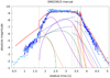 |
Fig. A.11 Manual solution for EN020615. Labels are the same as in Fig. 3. |
| In the text | |
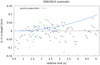 |
Fig. A.12 Length residuals of the automatic model for EN020615. Labels are the same as in Fig. 5. |
| In the text | |
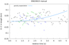 |
Fig. A.13 Length residuals of the manual model for EN020615. Labels are the same as in Fig. 5. |
| In the text | |
|
Fig. A.14 Automatic solution for EN180118 compared to radiometric and light-curve data. Labels are the same as in Fig. 3. |
| In the text | |
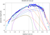 |
Fig. A.15 Manual solution for EN180118. Labels are the same as in Fig. 3. |
| In the text | |
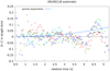 |
Fig. A.16 Length residuals of the automatic model for EN180118. Labels are the same as in Fig. 5. |
| In the text | |
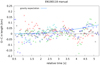 |
Fig. A.17 Length residuals of the manual model for EN180118. Labels are the same as in Fig. 5. |
| In the text | |
Current usage metrics show cumulative count of Article Views (full-text article views including HTML views, PDF and ePub downloads, according to the available data) and Abstracts Views on Vision4Press platform.
Data correspond to usage on the plateform after 2015. The current usage metrics is available 48-96 hours after online publication and is updated daily on week days.
Initial download of the metrics may take a while.