| Issue |
A&A
Volume 671, March 2023
|
|
|---|---|---|
| Article Number | A65 | |
| Number of page(s) | 15 | |
| Section | Planets and planetary systems | |
| DOI | https://doi.org/10.1051/0004-6361/202141784 | |
| Published online | 08 March 2023 | |
Effect of improved atmospheric opacities in modelling sub-Neptunes
A case study for GJ 1214 b
1
Centre for Astronomy and Astrophysics (ZAA), Technische Universität Berlin (TUB),
Hardenbergstr. 36,
10623
Berlin, Germany
e-mail: This email address is being protected from spambots. You need JavaScript enabled to view it.
2
Department of Extrasolar Planets and Atmospheres (EPA), Institute for Planetary Research (PF), German Aerospace Centre (DLR)
Rutherfordstr. 2,
12489
Berlin, Germany
e-mail: This email address is being protected from spambots. You need JavaScript enabled to view it.
3
Department of Planetary Physics, Institute for Planetary Research (PF), German Aerospace Centre (DLR)
Rutherfordstr. 2,
12489
Berlin, Germany
4
Institute for Geological Sciences, Planetology and Remote Sensing, Freie Universität Berlin (FUB),
Malteserstr. 74-100,
12249
Berlin, Germany
Received:
13
July
2021
Accepted:
12
September
2022
Abstract
Aims. We investigate the impact of updated atmospheric mean opacity input values on modelled transit radius and the distribution of interior layer mass fractions.
Methods. We developed and applied a coupled interior-atmosphere model. Our straightforward semi-grey calculation of atmospheric temperature enables us to perform thousands of model realisations in a Monte Carlo approach to address potential degeneracies in interior and atmospheric mass fraction. Our main constraints are planetary mass and radius from which our model infers distributions of the internal structure of exoplanetary classes ranging from Super-Earth to Mini-Neptune. We varied the relative masses of gas, envelope, mantle, and core layers subject to constraints on the bulk density from observations, and investigated the effect of updating atmospheric mean opacities.
Results. First, we validate our model output with observed temperature profiles for modern Neptune. We can reproduce the basic features in the middle atmosphere but not the temperature inversion in the upper layers, which is likely because our model lacks aerosol heating. Calculated interiors are generally consistent with modern Neptune. Second, we compare with the well-studied object GJ 1214 b and obtain results that are broadly consistent with previous findings; they suggest correlations between modelled gas, water, and core mass fractions, although these are generally weak. Updating the opacities leads to a change on the order of a few percent in the modelled transit radius. This is comparable in magnitude to the planned accuracy of the PLATO data for planetary radius, suggesting that the opacity update in the model is important to implement.
Key words: planets and satellites: individual: GJ 1214 b / planets and satellites: atmospheres / planets and satellites: composition / planets and satellites: fundamental parameters / planets and satellites: interiors
The Authors 2023
 Open Access article, published by EDP Sciences, under the terms of the Creative Commons Attribution License (https://creativecommons.org/licenses/by/4.0), which permits unrestricted use, distribution, and reproduction in any medium, provided the original work is properly cited.
This article is published in open access under the Subscribe to Open model. This email address is being protected from spambots. You need JavaScript enabled to view it. to support open access publication.
1 Introduction
The Kepler mission has suggested that sub-Neptunes are likely to be very common (Batalha 2014) with a wide range of masses and radii. Interior structures however are challenging to constrain since numerous, degenerate bulk compositions can fit the current data. Interior-atmosphere models that are both accurate and flexible are needed in order to explore these degeneracies and begin to quantify them. These degeneracies have now been investigated for over a decade; see for example Rogers & Seager (2010), Nettelmann et al. (2011), and Valencia et al. (2013) (who all focused on GJ 1214 b). Recently, several new studies have been published that use such models to investigate this issue (e.g. Dorn & Heng 2018; Madhusudhan et al. 2020; Kite & Barnett 2020). We address this topic by applying an interior-atmosphere coupled model that compares reasonably well with more complex schemes but can be applied over a wider parameter range. Our goal is to investigate the effect of improved atmospheric parameters in order to extend our knowledge of the interior structure of sub-Neptunes.
The PLATO mission (Rauer et al. 2014) will bring about a new age of planetary characterisation. Interpreting the forthcoming data will require next-generation interior-atmosphere models that are flexible enough to cover the wide parameter range (core, mantle, gas mass fractions, and compositions) yet sufficiently detailed to capture, for example, realistic atmospheric temperature profiles and therefore planetary radius contributions.
Regarding interior-atmosphere models with straightforward or isoprofile atmospheres, Noack et al. (2017) estimated atmospheric effects by indirectly adopting a scaling approach to calculate habitable zone (HZ) boundaries based on Kopparapu et al. (2013), taking as input incoming flux and atmospheric composition. Lopez & Fortney (2014) applied a lookup grid for atmospheric temperature with stellar flux and gravity as input in order to estimate mass-radius relations for sub-Neptunes. These authors applied an isothermal profile for their atmosphere, with a parameterization for the radius of the envelope and solid inner body. They investigated the effects of a wide range of planetary masses, gas mass fractions, and stellar fluxes in an effort to better characterise the mass-radius relationship for sub-Neptunes. With this isothermal profile, the radius of the atmosphere of their modelled planet grid is ≈0.1 RP. This approach neglects the effects of greenhouse heating for example, which increases the scale height and therefore the thickness of the atmosphere. In their relation, the top of the atmosphere is kept constant at an arbitrary pressure, whereas in reality the observed transit radius is a function of the atmospheric bulk properties.
Regarding atmosphere-interior models with semi-grey atmospheres, Dorn & Heng (2018) used the Guillot (2010) approximation to calculate temperature. Rogers & Seager (2010) used a broadly comparable model described in Hansen (2008). However, as their model input, these latter authors used a ratio of shortwave to longwave mean opacities (γ) based on earlier works (Freedman et al. 2008, hereafter F08) that is approximately one order of magnitude larger than the updated value in Freedman et al. (2014, hereafter F14). In general, γ values vary as a function of composition (e.g. steam, primary atmospheres) and pressure. Valencia et al. (2013), who modelled the bulk composition of sub-Neptunes, chose a mean opacity (κ) input value that yields 1000 K at 1 bar based on a line-by-line approach, and then employed an extrapolated analytical formula to vary the mean opacity with pressure, temperature, and metallicty.
Regarding complex climate-chemistry atmosphere-only models, numerous exoplanetary studies to date have applied such models to investigate for example potential habitability and atmospheric biosignatures (e.g. Segura et al. 2003, 2005; Hu & Seager 2014; Meadows et al. 2018; Madhusudhan et al. 2020; Scheucher et al. 2020; Wunderlich et al. 2020). There exist degeneracies in the atmosphere-interior composition based on mass–radius measurements alone. We note that transmission spectra, for example from the James Webb Space Telescope (JWST), will likely help to address such degeneracies.
GJ 1214 b (Charbonneau et al. 2009) is one of the most well-investigated sub-Neptunes in terms of both planetary interior and atmosphere. Observations generally suggest a degeneracy between either a higher metallicity atmosphere or the presence of equilibrium condensate such as clouds or photochemical hazes in order to account for the relatively flat transmission spectra (Kreidberg et al. 2014; Rackham et al. 2017; Crossfield & Kreidberg 2017; Gao & Benneke 2018; Kawashima et al. 2019; Lavvas et al. 2019). The non-detection of helium (Kasper et al. 2020) suggests the possible loss of the primary atmosphere. Various works have chosen to focus on the interior, assuming a relatively simple gas layer (Nettelmann et al. 2011) or modelling the atmosphere using a climate-only model (Charnay et al. 2015; Lavvas et al. 2019) and neglecting the interior altogether. Rogers & Seager (2010) and Valencia et al. (2013) applied atmosphere-interior models to GJ 1214 b but did not explore the effect of updating input parameters such as opacity.
A main motivation of the present work is to investigate the influence of input data updates in the mean opacities from F14 updated from F08 on the simulated atmosphere-interior over a wide parameter range for GJ 1214 b. These opacities are used as input in our modelled gas layer. We compare with output from other models in the literature that use the original opacity data. As GJ 1214 b is likely to have a substantial gas layer due to its low bulk density, employing updated opacities is especially important when accurately modelling the planetary structure.
This paper is structured as follows. Section 2 provides the model description, Sects. 3 and 4 present the validation and case study, Sect. 5 presents results for the effect of the opacity update, and Sect. 6 presents a summary of our conclusions. Supplementary figures and tables can be found in Appendices A and B, respectively.
2 Model description
Our interior-atmosphere model TATOOINE (Tool for ATmospheres, Outgassing, and Optimal INteriors of Exoplanets) splits the planet into multiple layers of distinct composition: an iron core, a silicate mantle, a water-ice shell, and a hydrogen-helium gas layer. These different layers are described individually below. The interior model was discussed in detail in Baumeister et al. (2020) and here we provide just a brief description. The gas layer is a new feature and is described and validated in this paper for the first time. The different layers are described individually below followed by a brief description of the interior model.
Our main assumptions are as follows. We calculate a stratified four-layer structure of distinct compositions in hydrostatic equilibrium, with Earth-like values for interior parameters such as the magnesium number (Mg#) and the Fe/Si ratio, with only one layer in the iron core and silicate mantle, and a water layer composed of pure H2O (as opposed to a mixture of for example water, methane, and ammonia). Our gas layer is grain-free (no clouds or hazes), assuming a straightforward climate (see below) with no interactive chemistry, and no convection in the semi-grey portion of the atmosphere. We also do not make use of any a priori information - from for example formation models - in choosing our various model input values (Fe/Si, Mg#, atmospheric composition, or mean molecular weight, etc.).
As input, the model takes the planetary mass, layer composition, equation of state (EoS), and the mass fraction of each layer. From there, the planet is split into 2000 spherical shells. Mass, pressure, and temperature are integrated from the top downward to the planet's centre. The model is iterated until the excess mass at the planet centre is less than the preset tolerance (1 × 10⁻⁶) between consecutive iterations. In order to fully characterise the inherently degenerate solution space, we perform a parameter study over a range of layer mass fractions. We adopt a Monte Carlo (MC) approach as described in the modelling method Sect. 2.3.
We analyse the results of the parameter study by selecting MC model outcomes where the calculated transit radius lies within the error range for the observed radius of the planet Robs ± σR. We then plot the posterior distribution of the mass fraction in each layer and calculate the median value where the errors are calculated at the 16% and 84% quantiles (see Figs. 1, 4, A.1 and Sect. 2.4). These median values are then used as input for the core, water, and gas mass fraction in order to construct individual profiles for each model realisation (e.g. Fig. A.2).
2.1 Gas layer
The modelled gas layer has two regions: an upper layer consisting of the irradiated semi-grey atmosphere whose radiative budget is dominated by instellation, and a lower, high-pressure solar composition envelope. The composition of the atmosphere is determined by equilibrium chemistry which is calculated in the present study by the NASA Chemical Equilibrium with Applications (CEA) model (McBride et al. 1992). The CEA model uses a descent Newton Raphson method to minimise Gibbs free energy and then calculate the composition at thermodynamic equilibrium (see Table B.1). Initial element abundances are calculated based on user-input metallicity. Data are calculated for 50 reference elements including species condensation. Further details of the method and references for the thermodynamical input tables are provided by McBride et al. (1992). We note that the mean opacities calculated by the Freedman studies mentioned above assume condensation of only primary species, unlike the CEA model which includes more complex condensation of secondary species. However. for the current work, we assume that the effects of this caveat are small for the rather modest range of metallicities considered. The energy budget of the radiative regime is determined on the one hand by photons emitted from the planetary interior below and on the other hand by heat release into the atmospheric region above. Within the envelope, there are two regimes: radiative and convective, the boundary of which is defined by the Schwarzschild criterion.
2.1.1 Irradiated atmosphere
In the irradiated atmosphere, we apply the radiative scheme of Guillot (2010) to calculate the temperature as a function of pressure for hydrogen-helium-dominated atmospheres using their Eq. (49). As input to the Guillot model, we provide the equilibrium temperature Teq (using an albedo of zero if not otherwise known) and the intrinsic temperature Tint, and γ = κvis/κth, where κvis and κth are the visible and thermal (Rosseland) mean opacities from F14, respectively. For each metallicity, the Rosseland mean opacities are provided as a table of look-up values along a grid of for example Plocal, Tlocal, Teff. The Rosseland mean opacity is defined as:
 (1)
(1)
where the wavelength-dependent opacity (κλ) is calculated for each point in the pressure-temperature grid, and the Planck function (Βλ) is weighted using either the local temperature for κth, or stellar effective temperature for κvis.
In this work, we employ Rosseland rather than Planck mean opacities in order that we may compare with earlier modelling studies such as that of Valencia et al. (2013). The Rosseland approach assigns a higher weighting at wavelengths contributing low opacities. It is therefore particularly suited to deep atmospheric regions where photon transport is approximately diffusional. However, the Guillot method used in our work employs a single opacity that is constant throughout the atmosphere. To our knowledge, there is no theory that suggests how to apply the Planck or the Rosseland mean over the entire profile in such a case. However, we note that, in reality, changing chemical composition and pressure over the atmospheric profile could lead to variations in the value of the Rosseland opacity. These caveats are a point of investigation for future work.
The data available for a given exoplanet is generally minimal, and so as a starting point we used Teq for Tlocal (with the associated Teff for κvis) because Teq can be derived observationally. We note that an aim of our work is to determine the effect of updating the original opacity data without the challenge of interpolating in p–T, which could introduce biases. For our model calculations, we therefore chose the closest available values in the input (pressure-temperature) opacity grid to our model scenarios (see below).
In the case of GJ 1214 b, we assume Teq = 555 K (assuming zero bond albedo) and a Teff = 3026 K (Charbonneau et al. 2009). The closest values in F14 are 575 K and 3000 K. For Neptune, we followed a similar procedure, but instead of using the observed Teq = 46 K from (Guillot 2005, bond albedo of 0.290), we used T1bar = 72 K, with Tlocal = 75 K and Teff = 6000 K being the closest value in F14. We adopted this approach because Neptune's radius is frequently defined at 1 bar (which is used here instead of the transit radius in our analysis; see Sect. 3).
While this approach lends itself to estimating a value for Plocal in the case of Neptune, for GJ 1214 b we compared the temperature profiles using mean opacity values of different Plocal to profiles from different literature sources (e.g. Miller-Ricci & Fortney 2010; Valencia et al. 2013) and selected the most consistent profile, namely Plocal = 0.1 bar. In cases where such comparison data are not available, Plocal could be allowed to vary as a free input parameter.
In our model, planetary radius is taken to be the transit radius following the methodology described in Guillot (2010) and defined as the pressure level where the chord optical depth in the visible range τch is equal to 0.56 (Lecavelier des Etangs et al. 2008). This quantity is related to the optical depth by:
 (2)
(2)
where H is the scale height and Rsolid is the total sum of the planetary thickness of the water, mantle, and core layers. We note that the temperature and scale height dependence can lead to a 30% decrease in the optical depth at the effective planetary radius for hot Jupiters compared with warm super-Earths such as GJ 1214 b.
2.1.2 High-pressure envelope
Sub-Neptune atmospheres can extend over a large range of temperature and pressure such that equations of state based on the ideal gas law can begin to break down in the deeper layers. In our work, in the high-pressure envelope, we use the EoS first described by Saumon et al. (1995) and expanded upon by Chabrier et al. (2019), hereafter collectively referred to as (SCvH).
The boundary condition between the irradiated gas layer (described above) and the underlying (radiative) envelope is determined by a pressure criterium similar to that applied by Jin et al. (2014). The switch occurs at a pressure level where incoming energy from the star has been absorbed and the main energy source is the thermal contribution of the planet; in other words, where τ ≫ 1. Using the relation in Rogers et al. (2011)  , we set the specific value of
  , which corresponds to a pressure level of approximately 10 bar. At greater pressures, the Guillot temperature and pressure are used as inputs for the non-ideal EoS density calculation as performed by SCvH. The temperature profile is calculated along the radiative gradient (∇rad) defined by Jin et al. (2014), as:
 (3)
(3)
where Tint is the planetary intrinsic temperature. This procedure continues until the convective regime is reached, as defined by the Schwarzschild criterium:
 (4)
(4)
whereby the advective gradient (Vad) in the SCvH table is compared with the radiative gradient stated above. Once this condition is reached, the entropy is fixed and the temperature and density are calculated isentropically. Appendix C discusses caveats associated with applying Eqs. (3) and (4) in the way described above.
2.2 Interior
We consider the following compositionally distinct layers in modelling the solid interior of each MC realisation: an iron core, a silicate mantle, and a water layer. We provide here a brief overview of the model assumptions. For more details on the model, see Baumeister et al. (2020).
The density of Earth's core suggests that it is not composed of pure iron, but that lighter alloying elements are present (Rubie et al. 2015). Even for Earth, and especially for exoplanets, the exact amount of these lighter alloys is not known well. Therefore, we follow an approach by Valencia et al. (2007) assuming a pure iron core and using a Mie-Grüneisen-Debye equation of state (Sotin et al. 2007) to calculate the density profile.
For the silicate mantle, we assume a pure composition of MgSiO3 perovskite (bridgmanite) for the entire mantle. We model the mantle with a Vinet EoS (Vinet et al. 1989) using the suggested parameters from Oganov et al. (2001). We allow all MC realisations to have an extended water layer above the silicate mantle to cover the possibility of 'water worlds' (Léger et al. 2004; Zeng et al. 2019). We employ the AQUA EoS (Haldemann et al. 2020), which spans a pressure-temperature range suitable for interior conditions and which calculates the density and adiabatic gradients based on a suite of H2O EoSs.
We do not consider temperature dependence for the silicate mantle or the iron core, because the associated change in radius contribution is negligibly small for our purposes here (Seager et al. 2007). Moreover, the planetary radius in our MC realisations is mainly determined by the extended hydrogen atmosphere and envelope, whereas changes in the solid interior contribute only as second-order effects. However, it should be noted that thermal effects can have a significant impact on the thickness of the water layer (Thomas & Madhusudhan 2016). As such, we use the following adiabatic gradient to calculate the temperature profile for the water layer:
 (5)
(5)
2.3 Modelling method
The model takes as a boundary parameter the total mass of the planet along with starting values for mass fractions of the core, water, and gas layers, with the remaining mass in the mantle. Using a Monte Carlo approach, we distribute 5000 models over this parameter space, where the solver varies the radius randomly within user-defined minimum and maximum values.
For each mass fraction combination of core, water, and gas (with the mantle making up the rest), the model begins by calculating the temperature profile. From this, the pressure and gravity profiles are calculated, which serve as input for the EoS of each layer when calculating the density profile. With the densities and planetary radii, the solver integrates the total mass for each layer until either the pressure (for the atmosphere-envelope boundary) or mass (for the core, water, and gas layers) boundary condition is reached. Once the solver has reached the centre of the planet, it adjusts the radius for the next iteration. If mass is left over, the model increases the radius in the next iteration, and vice versa. This continues until the variation between consecutive iterations is less than the tolerance.
On completion of the parameter study, the results are filtered based on their final radii such that only solutions whose transit radius lies within the assumed error range of the observations (typically 1000 from the 5000 model realisations in total) are used in the analysis. These solutions are then plotted in a 'corner plot' that shows the posterior distribution of each mass fraction. The median values of these distributions are calculated along with the values at the 84th and 16th quantiles (equivalent to ±1σ for a Gaussian distribution). These median values are used to generate individual profiles for each MC run and they serve as the basis for our comparison to investigate how the input atmospheric mean opacity values influence the interior structure. Table 1 shows the key input parameters for the planets simulated.
It should be noted in general that the median values and their error bars are calculated independently from one another, which is why the sum of the median mass fractions (core, mantle, water, and gas) is not equal to one. For this reason, choosing such combinations of median values does not represent a self-consistent interior solution found by the parameter study. Alternatively, one would choose an interior structure by selecting a specific value for either core, water, or gas in order to find the mass fraction of the other layers (see Sect. 4 for an example).
Model input parameters used in this work (refer to Sect. 2.1.1 regarding the mean opacity parameters).
2.4 Interpreting corner plots
Corner plots are useful for visualising how the distribution of solutions in a multi-variable parameter space vary with respect to one another, along with the independent distribution of solutions of each variable; see Fig. 1 for an example. In this work, we use the mass fractions (w) of each layer as free parameters. The histogram plots along the diagonal show the distribution of layer mass fractions that result in a valid solution. The contour plots show how each layer varies with respect to the other layers; that is, for a specific gas mass fraction, they show the allowed range of core, mantle, and water mass fractions. The contour plots have lines drawn at each σ level (with solid, dashed, and dotted lines corresponding to 1σ, 2σ, and 3σ, respectively) and feature multiple local minima throughout the parameter space.
We also denote the median value of each distribution as a solid vertical blue line, with the upper and lower bounds shown as vertical dashed blue lines calculated at the 84% and 16% quantiles, respectively. The median and its associated errors are written above each histogram.
3 Validation: Neptune
We consider modern Neptune to validate our atmosphere-interior model. While there are a number of caveats involved with this comparison (see below), our main aim here is to compare observed temperature profiles with those calculated by our semi-grey scheme for Neptune conditions in the upper-atmosphere irradiated regime. For this purpose, the validation is assumed to be appropriate. The main caveats are as follows:
Neptune's bulk mass lies just above the intended range of our (sub-Neptune) model. Furthermore, current Neptune interior models in the literature (e.g. Scheibe et al. 2019) generally apply a continuous interior modelling approach rather than a stratified planet with distinct layers as is the case in our model. As such, our model shows more variation in the final interior structures, with the "true" Neptune interior included within the range of our model output.
Our model water layer is composed of pure water, similarly to that of Scheibe et al. (2019), rather than a mixture of water, methane, and ammonia for example, as in Podolak et al. (1995).
The metallicity of our atmosphere is limited by the range available in our input opacity tables (F14). We use the highest available, [M/H] = 1.7 or 50× solar metallicity, although current estimates for Neptune suggest a value of ~80 ± 20× (Mousis et al. 2020).
Results are analysed using the radius at 1 bar as opposed to the transit radius. We assumed error bars of 5% for both the mass and radius, which we take to be representative of current sub-Neptune data.
With these caveats in mind, results from our model suggest a median gas mass fraction of 2.05 M⊕, with a range of 1.49–2.73 M⊕ (Fig. 1 bottom right hand plot: log wgas ≈ −0.92 = 17.147 × 10−0.92 − 2.05 M⊕). Our results correspond to the gas mass fraction calculated for Neptune models in the literature, that is, from 2.3 M⊕ to 3.45 M⊕ (Podolak et al. 1995; Scheibe et al. 2019), which is within our ± 1σ range. We used the value of 2.05 M⊕as an input for Neptune when modelled with the Chabrier et al. (2019) EoS based on previously published models that satisfy the gravity data for the second (J2) and fourth (J4) gravitational moments (Helled et al. 2020). The latter value was obtained based on the modelled output of J2 and J4 which compared best with Voyager observations of Neptune (renormalised from Owen et al. 1991). Although Neptune lies just above the mass range of exoplanets intended for our model, our results are nevertheless broadly consistent when compared to those obtained from more dedicated models.
Figure 1 presents corner plot results for the modern Neptune validation, which suggest left-skewed mass fraction distributions (top panels, blue lines) with reasonably constrained relations between the gas fraction and the other layers: wwater, mantle, and core (Fig. 1, bottom row) but with less constrained (more degenerate) relations for the remaining layers (Fig. 1, second and third rows). The tendency for the solutions to skew left towards smaller mass fractions is due to the increased number of possible layer combinations (where Σ wlayer,i = 1) that result in a valid solution.
Figure 2 compares the modelled temperature-pressure profile output from our study (blue-green solid line) with observed values (red solid line) derived from Marten et al. (2005, Fig. 1). In the upper region our model results are cooler than the observations whereas in the lower region our results are warmer. These difference mainly arise because we adopted a lower metallicity and because our model lacks aerosol heating.
To test the robustness of our results, we doubled the number of MC cases from 5000 to 10 000 and compared the resulting change in the layer mass fractions output. None of the mass fractions changed by more than a few percent, which suggests that the number of MC cases used is sufficient.
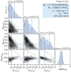 |
Fig. 1 Neptune corner plot showing the distribution of layer mass fractions (wlayer) for an assumed 50× metallicity atmosphere. Input values are shown in the light blue panel in the upper-right corner. Solid blue circles show median values. Error bars in the uppermost panels denote the 16th and 84th percentiles based on the distribution from the MC output. |
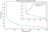 |
Fig. 2 Validation of the atmospheric pressure–temperature profile for Neptune with 50× metallicity using median values from Fig. 1 as our model input (solid green line). Observations taken from Fig. 1 of Marten et al. (2005) are plotted in red. |
 |
Fig. 3 Comparison of 1× solar pressure-temperature profile (this work, solid) with the model study of Valencia et al. (2013; dashed) and Miller-Ricci & Fortney (2010; dotted). |
4 Case study: GJ 1214 b
For the investigation of the atmosphere of GJ 1214 b, we compare our calculated pressure-temperature profile assuming 1× solar metallicity to the grain-free solar composition atmosphere in Valencia et al. (2013) and Miller-Ricci & Fortney (2010). For the interior validation, we compare with the model study of Rogers & Seager (2010).
4.1 Solar metallicity
Table B.2 lists the thermal mean opacity, κth, and visible mean opacity, κvis, from F14 as well as the associated γ (κvis/κth) value assumed in our work. Valencia et al. (2013) used the F08 mean opacities for their κth, and selected a γ value of 0.032 to give a temperature of 1000 K at 1 bar based on Miller-Ricci & Fortney (2010), which was kept fixed in their various scenarios. To select our κth and κvis we chose a scenario that was closest to that of Valencia et al. (2013) with γ = 0.0277, or a Plocal = 0.1 bar for a Tlocal = 575 K and a metallicity of 1 × solar.
Figure 3 suggests overall reasonable agreement between the modelled temperature profile from our work compared with that of the Valencia study, although there are some key differences. There is increased warming in our TATOOINE results in the upper and lower vertical sections due to the increased amounts of greenhouse gases (see Table B.1) included in our calculation of the mean opacities in F14 versus F08. We also include a high-pressure envelope in our atmosphere, which contributes to the divergence from Valencia et al. (2013) at the bottom of the atmosphere, because their work varied κ with pressure, temperature, and metallicity using extrapolated values.
Figure 3 also includes profiles generated in Miller-Ricci & Fortney (2010). Rather than a semi-grey approach as in Valencia et al. (2013) and Rogers & Seager (2010), Miller-Ricci & Fortney (2010) employed a full radiative-convective model. Our atmospheric pressure-temperature profile presented in Fig. 3 shows a better fit to the profile of Miller-Ricci & Fortney (2010) than that of Valencia et al. (2013) for pressures <1 bar, which suggests that our use of the updated mean opacity values leads to an improved comparison with more sophisticated models, which do not rely on such approximations. In order to further reduce the deviation at higher pressures, one likely solution is to use a combination of a pressure- and temperature-dependent κ, such as in Valencia et al. (2013), along with the inclusion of a high-pressure envelope.
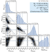 |
Fig. 4 Corner plot for GJ 1214 b showing the distribution of solutions for the parameter study with a 1× solar composition atmosphere (Table B.2). |
4.2 Interior structure
For our interior structure output, we compare with the model study of Rogers & Seager (2010). In their work, these authors investigated a variation of γ in the range 0.1–10. We note that they used the Planck mean opacity, while our work (and that of Valencia et al. 2013) uses the Rosseland mean (see discussion above).
In Fig. 4, the standard deviation of the solutions around the median wgas spans a range of over three orders of magnitude (0.18×10⁻³ − 0.62%). While this range is about an order of magnitude smaller than those suggested in Valencia et al. (2013) and Rogers & Seager (2010), we note that our work only makes use of the median values for our comparisons. These represent the most common points in the solution space or, in other words, the layer mass fractions for which there exists the largest number of degenerate solutions that fit the bulk planetary parameters. These solutions however do not necessarily represent the most physically likely.
If we refer to Fig. 4, and look at solutions where wwater → 0 in order to be comparable with the Valencia et al. (2013) study, the wgas spans a range of 10−2−10−1, approximately. For Table 2, we selected the parameter study solution with the smallest wwater. The associated wgas = 1.57% is in agreement with Valencia et al. (2013) for results where wwater ≈ 0.
Of the three cases discussed in Rogers & Seager (2010), their 'case I' is the most similar to our 1x solar composition atmosphere case and is chosen here for further investigation. For case I, their work shows gas mass fractions with a minimum range of 0.9 × 10⁻²−0.2% and a maximum range of 3.2−6.8%, depending on the atmospheric thermal profile when the mass and radius are allowed to vary within 1σ. While the minimum range is over all consistent with this work (0.18 × 10⁻³−0.62%), the difference in both the mean opacities and treatment of γ likely contributes to the difference in the upper range of solutions. While the Planck and Rosseland mean opacities converge at pressures higher than several tens of bar, the Planck mean opacity can be several orders of magnitude higher than the Rosseland value for pressures lower than ~ 1 bar depending on, for example, gas composition and temperature. Additionally, in their scenarios, γ is allowed to vary from 0.1 to 10.0 as a free parameter, while our γ value is kept fixed at 0.0277. These two factors likely account for their higher maximum gas mass fraction, which for our model is outside the ±1σ range of our results. To illustrate this point, the right hand column of Table 2 shows the parameter study solution with the greatest gas mass fraction, wgas = 3.96%, which is over 6.5σ from our median value.
GJ 1214 b layer mass-fraction solutions associated with the minimum wwater and maximum wgas from our parameter study for a 1× composition atmosphere.
4.3 Variation of metallicity
The atmospheric metallicity of GJ 1214 b is not well constrained. Miller-Ricci & Fortney (2010) assumed values ranging from 30x and 50× solar in addition to the 1 x case, whereas the model study by Drummond et al. (2018) assumed up to 100× solar. The observed [Fe/H] metallicity of the host star GJ 1214 is +0.39 ± 0.15 (Harpsøe et al. 2012), which corresponds approximately to 1.74×−3.46× solar values. While this does not necessarily correlate with the planetary atmospheric composition (in our own Solar System, Neptune has a composition equivalent to greater than 50× solar metallicity), it offers a starting value when no other information is available.
Other model studies, such as Dorn et al. (2015), used the stellar metallicity as an upper limit when modelling the Fe/Si and Mg/Si ratios as input for the core and mantle. However, the main focus of our work is the planetary gas layer, and therefore changes due to variations in the core and mantle were treated in a straightforward way: the Fe/Si and Mg# were kept fixed for all runs using Earth-like values (0.19 and 0.9, respectively) and their temperature dependence was not considered; this assumption has little effect (<100 km) on the final radius. Another possibility is to allow the atmospheric metallicity to vary as a free parameter, such as in Dorn & Heng (2018), although in our work we are limited by the range of metallicities available in F14. Valencia et al. (2013) used a combination of interpolation and analytical formulae to extrapolate mean opacity values for other metallicities and atmospheric compositions, which were found to be broadly consistent with the updated mean opacities used in our work. Applying a similar technique with such additional data would increase the range and flexibility of possible model scenarios.
We computed the atmospheric pressure-temperature profiles for all metallicities available in F14, and compared them to the profiles from Valencia et al. (2013) and Miller-Ricci & Fortney (2010; see Table B.2). Figure A.1 presents the corner plots for all metallicities, along with an aggregate corner plot that combines all the parameter study solutions for each metallicity. The median values for each metallicity are listed in Table B.3. A general trend can be seen in the corner plot distribution in Figs. 4 and A.1, where an increase in metallicity is associated with a decrease in gas mass fraction (e.g. Table B.4). As the metallicity increases, so too does the amount of constituent gases such as H2O, CO2, and CH4 (see Table B.1). This leads to additional warming in the atmosphere due to increased absorption, which increases the scale height and less gas mass is needed to fit a given planetary radius.
As can be seen in Fig. 5, while our model output agrees with the results of both Valencia et al. (2013) and Miller-Ricci & Fortney (2010) for the 1× case, the profiles deviate from Miller-Ricci & Fortney (2010) for the 30× and 50× metallicities. These differences likely arose for example because Miller-Ricci & Fortney (2010) employed a local-thermal-equilibrium model developed for irradiated exoplanets, which includes various atmospheric processes – such as convection - not included in our model for our upper atmosphere, only in the high-pressure envelope.
Employing the semi-grey approximation leads to a deviation of calculated atmospheric temperature from the equilibrium temperature of the planet. This arises due to, for example, greenhouse warming and the contribution from upwelling thermal radiation from the planetary interior. For Earth, the greenhouse component is of the order ~33 K at the surface. For our GJ 1214 b scenarios, the estimated equilibrium temperature is in the range of 393 to 555 K (Charbonneau et al. 2009). Our modelled TTran values by comparison range from ~490 to 760 K (see upper and lower dashed lines in Fig. 9 respectively). This difference of up to around 450 K between semi-grey and equilibrium temperatures reflects the importance of including accurate semi-grey schemes for sub-Neptunes.
To validate our interior results at higher metallicities, we compare with the so-called "Super-Earth" (SE) case in Rogers & Seager (2010). The most notable differences are the lack of He in their atmosphere, and the absence of a water layer in the planetary interior for their SE case. They calculated a gas mass fraction of 0.05%–1.2%. This is consistent with the gas mass fractions for higher metallicities (10×, 30×, and 50×) in Table B.4. The table suggests a trend with mostly a reduction in core mass fraction going from 3× to 50× metallicity. As the metallicity increases, the interior structure changes from a 'Mini-Neptune' with a large primordial atmosphere to a 'Super Earth' with a more modest gas mass fraction.
This trend is less apparent with the addition of a water layer, as can be seen in the corner plots in Fig. A.1 and Table B.3 for the median values of each mass fraction, along with their associated errors. While the same inverse relation between metallicity and gas fraction is still present, the resulting changes in the distributions for core, mantle, and water mass fractions are weaker. This suggests that it is challenging to constrain the interior based on our modelling results. Additional input constraints, such as from more sophisticated models or from other observed parameters (e.g. atmospheric spectral data or the Tidal love number k2), combined with more precise data (e.g. PLATO) are needed in order to be able to better resolve these degeneracies.
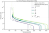 |
Fig. 5 Atmospheric pressure-temperature profiles and transit pressures (see Table B.3 for RTran values) for GJ 1214 b for all metallicities available in F14 (solid lines), compared with profiles from Valencia et al. (2013) and Miller-Ricci & Fortney (2010; dashed lines). See Fig. A.1 for the associated corner plots. |
5 Result, comparison of 2008 and 2014 mean opacities
We investigate here the influence of the updated F14 compared with the F08 mean opacity values for different γ values. We used both the γ quoted in Valencia et al. (2013), along with the γ from F14 used previously throughout this work (Table B.2), or = 0.032 and γFl4 ≈ 0.0277, respectively.
Comparing Fig. 4 with Fig. 6 suggests that while the changes due to the updated opacities are modest, they are more significant than the differences between Fig. 6a (γF08) and Fig. 6b (γF14). This suggests that variations in mean opacity values as individual input parameters have a greater impact on the final model output than changing γ = (κvis/κth) alone. This can also be seen in Table 3, which shows the change in each layer mass fraction and transit radius as a percentage difference.
Table 3 suggests that updating the opacities leads to an increase in the gas and water mass fractions, which is compensated by a decrease in the core and mantle mass fractions. This is different from the response discussed above (see Sect. 4.3) where increasing the metallicity led to a decrease in gas fraction due to heating through the atmosphere. The changes in Col. 1 compared to Col. 2, which demonstrate the effect of changing the mean opacities for each γ value, feature similar values of a few tens of percent. The values of Col. 3, which shows the effect of only changing γ when using the 2008 opacities, are approximately one order of magnitude smaller. This suggests that the effect of changing γ = κvis/κth is not large when compared to changes in κth and κvis. The transit radius, RR,Tran, changes by several tenths of a percent when using the median values and by up to a few percent for the specific (wcore, wwater, wgas) test case (marked with an asterisk in Table 3).
Figure 7 compares temperature profiles from our model (using different combinations of 2008 and 2014 κ and γ values) with other works in the literature. Our results using the updated opacities (solid purple line) lie closest to the profile from Miller-Ricci & Fortney (2010), compared to the profiles using the 2008 mean opacities, both from this model and that of Valencia et al. (2013). Updating the opacities leads to cooling in the middle atmospheric region, which leads to atmospheric contraction, which is why more gas is required to fit the observed planetary radius. This results in the increased gas mass fractions shown in Table 3.
Figure 7 suggests that the effect on PTran of using the 2014 values (solid circle symbol) compared with the 2008 values (cross symbol) is not large. However, we note that we are comparing median values derived from two large distributions. Many of the MC realisations using the 2008 opacities lead to solutions lying within the observed radius interval. This is also the case for the MC realisations using the 2014 opacities. Comparing the resulting two median values favours smaller differences due to averaging. It is more instructive to compare MC realisations away from the median, in order to gain insight into how large individual effects can be. In addition, the median values compared have different mass fractions, which are calculated independently for each of the layers. We therefore selected a case with a combination of (wcore, wwater, wgas) mass fraction which counted as a valid solution for the (κF08, γF08) case, and used this as input to generate the comparison profiles for (κF14, γF14) and (κF08, γF14). This case is marked with an asterisk in Table 3.
The percentage radius difference for (κF14, γF14) vs. (κF08, γF08) taken from Fig. 9 is equal to
 (6)
(6)
where RP is the observed radius of the planet (Table 1). We note that this difference results in the transit radius (solid circle) in Fig. 9, which was calculated using the updated opacity and γ values lying outside the quoted error bars, and as such would not be considered a valid solution in our analysis. See Table 3 for the remaining percentage values.
Figure 8 shows the corner plot solutions that are unique for the 2014 input values taken from Fig. 4 (shown in red) and for the 2008 input values taken from Fig. 6 (shown in blue), with the median (solid) and quantiles (dashed) listed separately in Table 4, along with the percentage changes. A similar comparison with (κF08, γF14) (not shown) did not differ significantly.
Figure 8 (bottom row) suggests a clear separation between a red (blue) region for lower (higher) core and mantle mass fractions and higher (lower) water and gas mass fractions. This behaviour is confirmed in the panels on the far right showing the mass fraction distributions.
Using Eq. (6), ΔRP,Tran ≈ 2.3% for solutions that are unique to each data set, or (κF14, γF14) XOR (κF08, γF08). While this difference is greater than the previous example of ~1.7% (see Fig. 9), which was calculated for only one value, it is still not significant when the measured radius precision is  (Charbonneau et al. 2009). However, compared to future missions, such as the upcoming PLATO mission, differences in planetary radii on the order of a few percent will be achievable (Rauer et al. 2014). Nevertheless, this result depends on numerous other factors, such as uncertain metallicity. However, we note that PLATO does not plan to observe GJ 1214 b. We also note that observations (Kreidberg et al. 2014) suggest a flat spectrum for GJ 1214 b, which is likely due to the presence of clouds, which are not included in our model. Even so, our results suggest that forthcoming data will nevertheless necessitate more accurate models with improved input parameters in order to be able to accurately interpret the results.
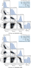 |
Fig. 6 Comparison of GJ 1214 b parameter study solutions for a 1× solar composition atmosphere using mean opacities from κF08 (F08), and either (a) γF08 (Valencia et al. 2013) or (b) γF14 (F14, Table B.2). |
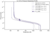 |
Fig. 7 Atmospheric temperature profiles for GJ 1214 b calculated using the median values from the parameter study runs in Fig. 4 (solid), Fig. 6a (thick dashed), and Fig. 6b (thick dash-dotted) compared to the profiles from Valencia et al. (2013; thin dashed) and Miller-Ricci & Fortney (2010; thin dotted). The transit pressures (PTran) are marked as solid symbols and the associated RTran values can be found in Table B.3. |
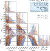 |
Fig. 8 Corner plot for GJ 1214 b showing the distribution of parameter study solutions that are unique to either (κF14, γF14) (shown in red) or (κF08, γF08; shown in blue) refer to Figs. 4 and 6, respectively. The associated median values and error bars for each layer are listed in Table 4. |
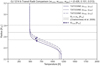 |
Fig. 9 Temperature profiles using both mean opacity databases and γ values for the selected (wcore, wwater, wgas) (see text) and the associated transit radius (see Table B.3 for RP,Tran values). The solid grey line denotes the observed planetary transit radius of GJ 1214 b, whereas the dashed lines represent the radius error bars in Charbonneau et al. (2009). |
6 Conclusions
The parameter space of sub-Neptunian exoplanets is large, covering a diverse range of interior-atmosphere solutions that are highly degenerate. Interior-atmosphere models must be flexible enough to investigate the large parameter space by balancing the accuracy of the results with the required computational time.
Our model, which uses the semi-grey approximation, produced results that are comparable with those of more sophisticated atmospheric models, while only requiring a fraction of the computational cost. This makes it possible to conduct thousands of model realisations, investigating the effect of a range of uncertain input parameters. By varying the metallicity as a proxy for the atmospheric composition, increased absorption of longwave radiation from the interior can raise the middle atmosphere temperature of GJ 1214 b by several hundred degrees compared with the equilibrium temperature. We note that there exist additional factors other than the input opacities, which can affect the calculated planetary transit radius. For example, the modelled atmospheric temperature profile is based on the planetary dayside of the planet, not on the terminator region where the transit radius is typically measured. Another factor is scattering in the visible and UV, which can lead to an increase in the determined transit radius. The use of additional data, such as observations over extended wavelength ranges, as well as constraints from spectral features, including the absorption bands of individual species and the Rayleigh slope (which constrains the atmospheric bulk molecular weight), can be used to constrain the atmospheric composition, potentially providing information about the planetary interior.
We find that varying the mean opacity had a larger effect on the distribution of interior solutions than varying γ. Degeneracies in the distribution of interior-atmosphere solutions cannot be constrained by the choice of atmosphere input parameters alone. Modest changes in the atmospheric gas fraction can lead to changes in transit radius that are of similar magnitude to the changes resulting from variations in the core and mantle mass fractions. The use of updated mean opacity and γ values in a semi-grey atmosphere results in improved calculations of temperature and transit radius when compared to studies that used older data. Such updates are needed for preparing the models for comparison with planned missions in exoplanet science.
Acknowledgements
This work has greatly benefited from the help, knowledge, and guidance of Dr. Mareike Godolt in the years leading up to its publication. We also appreciate the helpful discussions with Dr. Nadine Nettlemann, particularly with regard to Neptune. The authors acknowledge the support of the DFG Priority Program SPP 1992 "Exploring the Diversity of Extrasolar Planets" (GO 2610/2-1, TO 704/3-1). P. Baumeister and N. Tosi also acknowledge support from the DFG Research Unit FOR 2440 "Matter under planetary interior conditions" project number (PA 3689/1-1).
Appendix A Figures
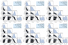 |
Fig. A.1 Corner plots for GJ 1214 b showing the distribution of interior solutions for each atmospheric metallicity as shown in Table B.2. The 1x metallicity plot is shown in Sect. 4.2, Fig. 4. The bottom right panel is an aggregate plot that includes the solutions from all metallicities. See Table B.3 for median values. |
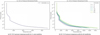 |
Fig. A.2 GJ 1214 b pressure-temperature profiles over the full model domain calculated using the median values of (wcore,wwater,wgas) as input (Fig. 4, Fig. A.1, Table B.3). |
Appendix B Tables
Mole fractions of atmospheric species for different metallicities.
Table of the Rosseland mean opacity values used for Neptune and GJ 1214 b taken from F14.
Comparison of solutions with either (a) the minimum wwater or (b) the maximum wgas for all metallicities.
Appendix C Caveats to temperature profile calculation
Here we discuss caveats relevant to calculating the temperature profile through the atmospheric regions from top to bottom:
Upper radiative regime
The central equation is taken from Guillot (2010), their equation 49. This is derived by imposing energy balance between incoming (stellar) and outgoing (planetary) radiation and assumes a mean opacity in the visible (κvis) and mean opacity from intrinsic heating in the infrared (κth). Emission from the atmosphere is assumed to have a negligible contribution to visible wavelengths. The methodic employs the Eddington approximation, assuming a static plane-parallel atmosphere in local thermodynamic equilibrium. The Guillot equation was originally derived in the context of hot Jupiters (HJs) and was applied at the time to HD 209458 b, for example. However, in our work, we simulate somewhat smaller, cooler objects such as GJ 1214 b. Table C.1 therefore compares caveat-relevant planetary and stellar data for HD 209458 b and GJ 1214 b.
Table C.1 suggests higher Teq and Tint by factors of 3 and 4 for the HJ case. Planetary radius is about a factor 6 smaller for the SE case which degrades somewhat the plane-parallel assumption mentioned above. Gravity is broadly similar for the two cases in Table C.1. Kappa values are also broadly similar for the two objects considered in Table C.1. In general atmospheric hazes could change κvis depending on particle radius whereas enhanced water vapour on super-Earths would likely lead to increased κth values.
Switch-over from ideal to non-ideal density calculation
In our work we define a switchover boundary at  which corresponds to about p>10 bar. At greater pressures, it is necessary to employ a non-ideal calculation of density. For this calculation, we use the SCvH non-ideal equation of state which yields density from a lookup table and requires temperature and pressure as input. Knowing for example the density and the volume of the gas layer enables calculation of the mass fraction, which is an output diagnostic in our cornerplots.
Radiative versus diffusional regime
A caveat of our work is that, at the switchover point of p>10 bar, we not only switch to a non-ideal density calculation but also apply equation (3) (hereafter 'the diffusional approximation') with increasing pressure for the temperature calculation until the convective regime is reached as defined by the Schwarzschild criterium. However, the diffusional approximation implicitly assumes that the radiative transfer of photons at high pressure arising from the planetary interior is limited by diffusion. However, a preferable approach which we note for future work would be to continue using the Guillot equation for temperature because this equation converges to the same solution as the diffusional approximation at high pressure. The convergence pressure depends for example on the internal temperature whereby higher internal temperatures lead to convergence at lower pressures. We now investigate the effect of this and other caveats.
The two panels (Fig. C1a and C1b) below show a range of temperature profiles for GJ 1214 b for the control run (for more details of this run see our Figure 3 above and the associated text). The left panel shows the effect of varying Teq and Tint over their uncertainty range. This panel shows cooling of about 140K in the upper atmosphere radiative regime upon reducing Teq from 555 K (control) to 393 K and an increase in lower atmosphere temperatures by up to several hundred degrees while increasing Tint from 24 K (control) to 50 K. The right panel shows the effect of switching from the Guillot temperature to the diffusional approximation temperature at pressures greater than 10 bar where considerably larger temperatures are calculated by the diffusional approximation in the deep atmosphere.
Planetary and stellar parameters for HD 209458 b and GJ 1214 b. *Upper limit. Values are taken from references in this work (section 4) and from Guillot (2010) and references therein.
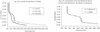 |
Fig. C.1 Effect upon modelled temperature of varying uncertain input parameters for the GJ1214b control run. The left panel shows Guillot temperature profiles for the control run (internal T of 24K, equilibrium T of 555K (dotted line with crosses); control but with internal T of 50K (dashed line with open circles) and control but with an equilibrium T of 393K (solid line with vertical bars). The right panel shows temperature profiles using the Guillot equation over all pressures (dotted line with crosses) compared with using Guillot down to p=10 bar and the diffusional approximation at higher p (solid line with open squares). |
References
- Batalha, N. M. 2014, PNAS, 111, 12647 [NASA ADS] [CrossRef] [Google Scholar]
- Baumeister, P., Padovan, S., Tosi, N., et al. 2020, ApJ, 889, 42 [Google Scholar]
- Chabrier, G., Mazevet, S., & Soubiran, F. 2019, ApJ, 872, 51 [NASA ADS] [CrossRef] [Google Scholar]
- Charbonneau, D., Berta, Z. K., Irwin, J., et al. 2009, Nature, 462, 891 [NASA ADS] [CrossRef] [Google Scholar]
- Charnay, B., Meadows, V., Misra, A., Leconte, J., & Arney, G. 2015, ApJ, 813, L1 [NASA ADS] [CrossRef] [Google Scholar]
- Crossfield, I. J. M., & Kreidberg, L. 2017, AJ, 154, 261 [Google Scholar]
- Dorn, C., & Heng, K. 2018, ApJ, 853, 64 [Google Scholar]
- Dorn, C., Khan, A., Heng, K., et al. 2015, A & A, 577, A83 [NASA ADS] [CrossRef] [EDP Sciences] [Google Scholar]
- Drummond, B., Mayne, N. J., Baraffe, I., et al. 2018, A & A, 612, A105 [NASA ADS] [CrossRef] [EDP Sciences] [Google Scholar]
- Freedman, R. S., Marley, M. S., & Lodders, K. 2008, ApJS, 174, 504 [NASA ADS] [CrossRef] [Google Scholar]
- Freedman, R. S., Lustig-Yaeger, J., Fortney, J. J., et al. 2014, ApJS, 214, 25 [CrossRef] [Google Scholar]
- Gao, P., & Benneke, B. 2018, ApJ, 863, 165 [CrossRef] [Google Scholar]
- Guillot, T. 2005, Annu. Rev. Earth Planet. Sci., 33, 493 [Google Scholar]
- Guillot, T. 2010, A & A, 520, A27 [NASA ADS] [CrossRef] [EDP Sciences] [Google Scholar]
- Haldemann, J., Alibert, Y., Mordasini, C., & Benz, W. 2020, A & A, 643, A105 [NASA ADS] [CrossRef] [EDP Sciences] [Google Scholar]
- Hansen, B. M. S. 2008, ApJS, 179, 484 [NASA ADS] [CrossRef] [Google Scholar]
- Harpsøe, K. B. W., Hardis, S., Hinse, T. C., et al. 2012, A & A, 549, A10 [Google Scholar]
- Helled, R., Nettelmann, N., & Guillot, T. 2020, Space Sci. Rev., 216 [Google Scholar]
- Hu, R., & Seager, S. 2014, ApJ, 784, 63 [Google Scholar]
- Jin, S., Mordasini, C., Parmentier, V., et al. 2014, ApJ, 795, 65 [Google Scholar]
- Kasper, D., Bean, J. L., Oklopcic, A., et al. 2020, AJ, 160, 258 [NASA ADS] [CrossRef] [Google Scholar]
- Kawashima, Y., Hu, R., & Ikoma, M. 2019, ApJ, 876, L5 [Google Scholar]
- Kite, E. S., & Barnett, M. 2020, PNAS, 117, 18264 [NASA ADS] [CrossRef] [Google Scholar]
- Kopparapu, R. K., Ramirez, R., & Kasting, J. F. 2013, ApJ, 765, 131; Erratum: 770, 82 [NASA ADS] [CrossRef] [Google Scholar]
- Kreidberg, L., Bean, J. L., Désert, J.-M., et al. 2014, Nature, 505, 69 [Google Scholar]
- Lavvas, P., Koskinen, T., Steinrueck, M. E., Muñoz, A. G., & Showman, A. P. 2019, ApJ, 878, 118 [NASA ADS] [CrossRef] [Google Scholar]
- Lecavelier des Etangs, A., Vidal-Madjar, A., Désert, J.-M., & Sing, D. 2008, A & A, 485, 865 [CrossRef] [EDP Sciences] [Google Scholar]
- Léger, A., Selsis, F., Sotin, C., et al. 2004, Icarus, 169, 499 [Google Scholar]
- Lopez, E. D., & Fortney, J. J. 2014, ApJ, 792, 1 [Google Scholar]
- Madhusudhan, N., Nixon, M. C., Welbanks, L., Piette, A. A. A., & Booth, R. A. 2020, ApJ, 891, L7 [Google Scholar]
- Marten, A., Matthews, H. E., Owen, T., et al. 2005, A & A, 429, 1097 [NASA ADS] [CrossRef] [EDP Sciences] [Google Scholar]
- McBride, B. J., & Gordon, S. 1992, Computer Program for Calculating and Fitting Thermodynamic Functions, NASA reference publication 1271 (National Aeronautics and Space Administration, Office of Management, Scientific and Technical Information Program) [Google Scholar]
- Meadows, V. S., Reinhard, C. T., Arney, G. N., et al. 2018, Astrobiology, 18, 630 [Google Scholar]
- Miller-Ricci, E., & Fortney, J. J. 2010, ApJ, 716, L74 [NASA ADS] [CrossRef] [Google Scholar]
- Mousis, O., Aguichine, A., Atkinson, D. H., et al. 2020, Space Sci. Rev., 216 [Google Scholar]
- Nettelmann, N., Fortney, J. J., Kramm, U., & Redmer, R. 2011, ApJ, 733, 2 [NASA ADS] [CrossRef] [Google Scholar]
- Noack, L., Rivoldini, A., & Van Hoolst, T. 2017, Phys. Earth Planet. Inter., 269 [Google Scholar]
- Oganov, A. R., Brodholt, J. P., & Price, G. D. 2001, Nature, 411, 934 [CrossRef] [Google Scholar]
- Owen, W. M., Vaughan, R. M., & Synnott, S. P. 1991, AJ, 101, 1511 [NASA ADS] [CrossRef] [Google Scholar]
- Podolak, M., Weizman, A., & Marley, M. 1995, Planet. Space Sci., 43, 1517 [NASA ADS] [CrossRef] [Google Scholar]
- Rackham, B., Espinoza, N., Apai, D., et al. 2017, ApJ, 834, 151 [Google Scholar]
- Rauer, H., Catala, C., Aerts, C., et al. 2014, Exp. Astron., 38, 249 [Google Scholar]
- Rogers, L. A., & Seager, S. 2010, ApJ, 716, 1208 [NASA ADS] [CrossRef] [Google Scholar]
- Rogers, L. A., Bodenheimer, P., Lissauer, J. J., & Seager, S. 2011, ApJ, 738, 59 [NASA ADS] [CrossRef] [Google Scholar]
- Rubie, D., Jacobson, S., Morbidelli, A., et al. 2015, Icarus, 248, 89 [NASA ADS] [CrossRef] [Google Scholar]
- Saumon, D., Chabrier, G., & van Horn, H. M. 1995, ApJS, 99, 713 [NASA ADS] [CrossRef] [Google Scholar]
- Scheibe, L., Nettelmann, N., & Redmer, R. 2019, A & A, 632, A70 [NASA ADS] [CrossRef] [EDP Sciences] [Google Scholar]
- Scheucher, M., Wunderlich, F., Grenfell, J. L., et al. 2020, ApJ, 898, 44 [Google Scholar]
- Seager, S., Kuchner, M., Hier-Majumder, C., & Militzer, B. 2007, ApJ, 669, 1279 [Google Scholar]
- Segura, A., Krelove, K., Kasting, J. F., et al. 2003, Astrobiology, 3, 689 [NASA ADS] [CrossRef] [Google Scholar]
- Segura, A., Kasting, J. F., Meadows, V., et al. 2005, Astrobiology, 5, 706 [Google Scholar]
- Sotin, C., Grasset, O., & Mocquet, A. 2007, Icarus, 191, 337 [Google Scholar]
- Thomas, S. W., & Madhusudhan, N. 2016, MNRAS, 458, 1330 [CrossRef] [Google Scholar]
- Valencia, D., Sasselov, D. D., & O'Connell, R. J. 2007, ApJ, 656, 545 [NASA ADS] [CrossRef] [Google Scholar]
- Valencia, D., Guillot, T., Parmentier, V., & Freedman, R. S. 2013, ApJ, 775, 10 [NASA ADS] [CrossRef] [Google Scholar]
- Vinet, P., Rose, J. H., Ferrante, J., & Smith, J. R. 1989, J. Phys.: Condensed Matter, 1, 1941 [NASA ADS] [CrossRef] [Google Scholar]
- Wunderlich, F., Scheucher, M., Godolt, M., et al. 2020, ApJ, 901, 126 [Google Scholar]
- Zeng, L., Jacobsen, S. B., Sasselov, D. D., et al. 2019, PNAS, 116, 9723 [Google Scholar]
All Tables
Model input parameters used in this work (refer to Sect. 2.1.1 regarding the mean opacity parameters).
GJ 1214 b layer mass-fraction solutions associated with the minimum wwater and maximum wgas from our parameter study for a 1× composition atmosphere.
Table of the Rosseland mean opacity values used for Neptune and GJ 1214 b taken from F14.
Comparison of solutions with either (a) the minimum wwater or (b) the maximum wgas for all metallicities.
Planetary and stellar parameters for HD 209458 b and GJ 1214 b. *Upper limit. Values are taken from references in this work (section 4) and from Guillot (2010) and references therein.
All Figures
|
Fig. 1 Neptune corner plot showing the distribution of layer mass fractions (wlayer) for an assumed 50× metallicity atmosphere. Input values are shown in the light blue panel in the upper-right corner. Solid blue circles show median values. Error bars in the uppermost panels denote the 16th and 84th percentiles based on the distribution from the MC output. |
| In the text | |
|
Fig. 2 Validation of the atmospheric pressure–temperature profile for Neptune with 50× metallicity using median values from Fig. 1 as our model input (solid green line). Observations taken from Fig. 1 of Marten et al. (2005) are plotted in red. |
| In the text | |
|
Fig. 3 Comparison of 1× solar pressure-temperature profile (this work, solid) with the model study of Valencia et al. (2013; dashed) and Miller-Ricci & Fortney (2010; dotted). |
| In the text | |
|
Fig. 4 Corner plot for GJ 1214 b showing the distribution of solutions for the parameter study with a 1× solar composition atmosphere (Table B.2). |
| In the text | |
|
Fig. 5 Atmospheric pressure-temperature profiles and transit pressures (see Table B.3 for RTran values) for GJ 1214 b for all metallicities available in F14 (solid lines), compared with profiles from Valencia et al. (2013) and Miller-Ricci & Fortney (2010; dashed lines). See Fig. A.1 for the associated corner plots. |
| In the text | |
|
Fig. 6 Comparison of GJ 1214 b parameter study solutions for a 1× solar composition atmosphere using mean opacities from κF08 (F08), and either (a) γF08 (Valencia et al. 2013) or (b) γF14 (F14, Table B.2). |
| In the text | |
|
Fig. 7 Atmospheric temperature profiles for GJ 1214 b calculated using the median values from the parameter study runs in Fig. 4 (solid), Fig. 6a (thick dashed), and Fig. 6b (thick dash-dotted) compared to the profiles from Valencia et al. (2013; thin dashed) and Miller-Ricci & Fortney (2010; thin dotted). The transit pressures (PTran) are marked as solid symbols and the associated RTran values can be found in Table B.3. |
| In the text | |
|
Fig. 8 Corner plot for GJ 1214 b showing the distribution of parameter study solutions that are unique to either (κF14, γF14) (shown in red) or (κF08, γF08; shown in blue) refer to Figs. 4 and 6, respectively. The associated median values and error bars for each layer are listed in Table 4. |
| In the text | |
|
Fig. 9 Temperature profiles using both mean opacity databases and γ values for the selected (wcore, wwater, wgas) (see text) and the associated transit radius (see Table B.3 for RP,Tran values). The solid grey line denotes the observed planetary transit radius of GJ 1214 b, whereas the dashed lines represent the radius error bars in Charbonneau et al. (2009). |
| In the text | |
|
Fig. A.1 Corner plots for GJ 1214 b showing the distribution of interior solutions for each atmospheric metallicity as shown in Table B.2. The 1x metallicity plot is shown in Sect. 4.2, Fig. 4. The bottom right panel is an aggregate plot that includes the solutions from all metallicities. See Table B.3 for median values. |
| In the text | |
|
Fig. A.2 GJ 1214 b pressure-temperature profiles over the full model domain calculated using the median values of (wcore,wwater,wgas) as input (Fig. 4, Fig. A.1, Table B.3). |
| In the text | |
|
Fig. C.1 Effect upon modelled temperature of varying uncertain input parameters for the GJ1214b control run. The left panel shows Guillot temperature profiles for the control run (internal T of 24K, equilibrium T of 555K (dotted line with crosses); control but with internal T of 50K (dashed line with open circles) and control but with an equilibrium T of 393K (solid line with vertical bars). The right panel shows temperature profiles using the Guillot equation over all pressures (dotted line with crosses) compared with using Guillot down to p=10 bar and the diffusional approximation at higher p (solid line with open squares). |
| In the text | |
Current usage metrics show cumulative count of Article Views (full-text article views including HTML views, PDF and ePub downloads, according to the available data) and Abstracts Views on Vision4Press platform.
Data correspond to usage on the plateform after 2015. The current usage metrics is available 48-96 hours after online publication and is updated daily on week days.
Initial download of the metrics may take a while.