| Issue |
A&A
Volume 670, February 2023
Solar Orbiter First Results (Nominal Mission Phase)
|
|
|---|---|---|
| Article Number | L3 | |
| Number of page(s) | 8 | |
| Section | Letters to the Editor | |
| DOI | https://doi.org/10.1051/0004-6361/202245431 | |
| Published online | 27 January 2023 | |
Letter to the Editor
Signatures of dynamic fibrils at the coronal base: Observations from Solar Orbiter/EUI⋆
1
Max Planck Institute for Solar System Research, Justus-von-Liebig-Weg 3, 37077 Göttingen, Germany
e-mail: This email address is being protected from spambots. You need JavaScript enabled to view it.
2
School of Space Research, Kyung Hee University, Yongin, Gyeonggi 446-701, Republic of Korea
3
Physikalisch-Meteorologisches Observatorium Davos, World Radiation Center, 7260 Davos Dorf, Switzerland
4
ETH-Zürich, Wolfgang-Pauli-Str. 27, 8093 Zürich, Switzerland
5
Solar-Terrestrial Centre of Excellence – SIDC, Royal Observatory of Belgium, Ringlaan -3- Av. Circulaire, 1180 Brussels, Belgium
6
Université Paris-Saclay, CNRS, Institut d’Astrophysique Spatiale, 91405 Orsay, France
7
Skobeltsyn Institute of Nuclear Physics, Moscow State University, 119992 Moscow, Russia
8
UCL-Mullard Space Science Laboratory, Holmbury St. Mary, Dorking, Surrey RH5 6NT, UK
9
Lockheed Martin Solar and Astrophysics Laboratory, Building 252, 3251 Hanover Street, Palo Alto, CA 94304, USA
10
Bay Area Environmental Research Institute, NASA Research Park, Mailstop 18-4, Moffett Field, CA 94035, USA
11
CSIRO, Cnr Vimiera & Pembroke Roads, Marsfield, NSW 2122, Australia
Received:
10
November
2022
Accepted:
9
December
2022
Abstract
The solar chromosphere hosts a wide variety of transients, including dynamic fibrils (DFs) that are characterised as elongated, jet-like features seen in active regions, often through Hα diagnostics. So far, these features have been difficult to identify in coronal images, primarily due to their small size and the lower spatial resolution of the current extreme-ultraviolet (EUV) imagers. Here we present the first unambiguous signatures of DFs in coronal EUV data using high-resolution images from the Extreme Ultraviolet Imager (EUI) on board Solar Orbiter. Using the data acquired with the 174 Å High Resolution Imager (HRIEUV) of EUI, we find many bright dot-like features (with a size of 0.3−0.5 Mm) that move up and down (often repeatedly) in the core of an active region. In a space-time map, these features produce parabolic tracks akin to the chromospheric observations of DFs. Properties such as their speeds (14 km s−1), lifetime (332 s), deceleration (82 m s−2), and lengths (1293 km) are also reminiscent of the chromospheric DFs. The EUI data strongly suggest that these EUV bright dots are basically the hot tips (of the cooler chromospheric DFs) that could not be identified unambiguously before because of a lack of spatial resolution.
Key words: Sun: magnetic fields / Sun: UV radiation / Sun: corona / Sun: atmosphere
Movie associated to Fig. 1 is available at https://www.aanda.org/
© The Authors 2023
 Open Access article, published by EDP Sciences, under the terms of the Creative Commons Attribution License (https://creativecommons.org/licenses/by/4.0), which permits unrestricted use, distribution, and reproduction in any medium, provided the original work is properly cited.
This article is published in open access under the Subscribe-to-Open model.
Open Access funding provided by Max Planck Society.
1. Introduction
Dynamic fibrils (DFs), the thin jet-like on-disc features, are typically observed through Hα diagnostics of the solar chromosphere (Rutten 2007). They usually have a lifetime of 2−4 min and lengths between 1 and 4 Mm (De Pontieu et al. 2005). A combination of observations and numerical simulations strongly suggests that DFs are basically shock-driven phenomena (De Pontieu et al. 2005; Hansteen et al. 2006). Magnetoacoustic waves that leak from the lower atmosphere are guided upwards by magnetic fields and they form shocks at chromospheric heights. These shocks then catapult chromospheric material upwards and produce jet-like DFs (Heggland et al. 2007). In a space-time (X-T) diagram, these DFs generate characteristic parabolic tracks that are a result of their up-and-down motion (Hansteen et al. 2006; De Pontieu et al. 2007). Interestingly, these properties are similar to those of other solar features such as type-I spicules (off-limb features) or quiet-Sun mottles (on-disc features) and, indeed, studies (e.g. Rouppe van der Voort et al. 2007; Heggland et al. 2007) have shown that all of these different features are most probably a manifestation of a common underlying family of drivers related to shocks (De Pontieu et al. 2004).
Thus far, observations of DFs have mostly been restricted to the chromosphere (e.g. Hα observations) and transition region (e.g. IRIS1 observations). Extreme-ultraviolet (EUV) observations of DFs using coronal imagers such as the Atmospheric Imaging Assembly (AIA; Lemen et al. 2012) have particularly been hindered by their inadequate spatial resolution. For example, Skogsrud et al. (2016) studied the evolution of DFs using co-ordinated SST2, IRIS, and AIA data and found that the ‘bright rim’ visible on top of a DF in IRIS 1400 Å channel images cannot be unambiguously identified in AIA channels due to their lower spatial resolution.
In the present work, for the first time, we present unambiguous EUV signatures of such bright rims using high-resolution, high-cadence EUV observations from Solar Orbiter (Müller 2020). We describe the data in Sect. 2, whereas Sect. 3 outlines the results. Finally we conclude by summarising our results in Sect. 4.
2. Data
We use EUV imaging data from the Extreme Ultraviolet Imager (EUI; Rochus et al. 2020) on board Solar Orbiter. This particular dataset was taken by the 174 Å High Resolution Imager (HRIEUV) of EUI on 2022 March 7, between 00:35:06 and 02:14:02 UT, with a cadence of 5 s (part of the SolO/EUI Data Release 5.0; Mampaey et al. 2022). At the time of this observation, Solar Orbiter was located at a distance of 0.50 AU from the Sun. This results in the EUI plate scale being 178 km per pixel on the Sun. To remove the effect of jitter from the EUI images, we employed a cross-correlation-based image-alignment technique similar to the one described in Mandal et al. (2022).
During this observation, Solar Orbiter was almost aligned with the Sun-Earth line (with the angle spanned by Solar Orbiter, the Earth, and the Sun being −0.58°). This allowed us to use co-temporal and co-spatial data from the Solar Dynamics Observatory (SDO; Pesnell et al. 2012). In particular, we used EUV images from the 171 Å channel of the Atmospheric Imaging Assembly (AIA; Lemen et al. 2012) and the line-of-sight (LOS) magnetograms from the Helioseismic and Magnetic Imager (HMI; Scherrer et al. 2012), both onboard SDO. Although AIA 171 Å and EUI 174 Å passbands image plasma at comparable temperatures, the spatial resolution of AIA is significantly lower (plate scale of 0.6″ or 435 km on the Sun). To support the EUI observations3, AIA was running a special campaign at a 6 s (twice its nominal 12 s) cadence with half of its EUV channels (using only 131, 171, 193, and 304 Å). This high-cadence sequence was interrupted every 96 s (i.e. one out of every 16 frames) in order to obtain synoptic, full-disc images.
The EUI and SDO data were aligned using a combination of FITS keywords and visual inspection. This is sufficient for the current study because we only used the AIA data for qualitative comparisons. Lastly, while comparing the AIA and EUI data, we took the difference in light travel times between Sun-EUI and Sun-AIA into account. All the times that we quote in the Letter are times at 1 AU.
3. Results
In order to identify the DFs and to quantify their properties, we located them in the EUI movie and investigated their evolution using X-T diagrams. Figure 1a presents a snapshot from the EUI dataset which primarily encompasses the active region (AR) NOAA12960. In and around this AR, we find typical coronal structures such as closed loops, moss regions, fan loops, and jets. A closer look at the event movie (available online) reveals the ubiquitous presence of tiny bright blob-like or front-like structures that move back and forth with time. These are the features that we refer to as the EUV signatures of DFs4 and they are the subject of this study.
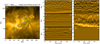 |
Fig. 1. Overview of the observed active region (AR). Panel a: sub-section of the HRIEUV full field of view from 2022 March 7. The boxes in various colours represent the artificial slits that we used to derive space-time (X-T) maps, some of which are shown in panels b−g. These X-T maps were contrast enhanced by performing a boxcar smooth subtraction along the space axis. The arrows drawn on every slit point to the increasing y-axis of the corresponding X-T maps. An animated version of this figure is available online. |
3.1. Capturing the EUV dynamic fibrils
In order to capture the observed motions of these DFs, we generated multiple X-T maps by placing artificial slits at several locations as shown in Fig. 1a. Each slit is 14 pixels wide and the final X-T maps were generated after averaging over these 14 pixels. Moreover, to highlight the bright tracks, we performed a boxcar (of 20 pixels) smooth subtraction along the transverse direction (i.e. along the y-axis) in each of these X-T maps.
In this overview figure (Fig. 1), names of the slits that are closer to the leading sunspot of the AR start with an S (for spot) and the ones that are away from it, overlying the moss regions, start with an M (for moss). Through this slit arrangement, we aim to cover a variety of magnetic environments. For example, slit S1 lies between two closed loops, slit S4 lies along a fan loop, slit M1 overlies a moss region close to the spot, whereas slits M2, M3, and M4 are also on moss regions but away from the leading spot in the AR. Panels b–g in Fig. 1 present six out of the eight X-T maps that we have derived.
Already, at a first glance, all of these X-T maps (except panel g) contain bright tracks that appear to have parabolic shapes. Furthermore, many of these tracks are also repetitive. As mentioned earlier, these are basically the signatures of dynamic fibrils that move up and down along the slits. Before we go on to examine these parabolic tracks in detail, we briefly discuss the slit-S4 X-T map (panel g). This map does not contain any parabolic tracks, but rather it only shows straight, periodic slanted ridges. These straight ridges are manifestations of the slow magneto-acoustic waves that propagate along the magnetic field (e.g. Krishna Prasad et al. 2012). In fact, such slanted ridges can also be seen in the bottom parts of the S1 (Fig. 1b) and S2 (Fig. 1c) maps.
In each X-T map, we fitted the individual seemingly parabolic bright tracks with a parabola and derived parameters such as deceleration, maximum speed (during ascent or descent) as well as maximum length (also referred as ‘height’ in the literature), and lifetime. The fitted parabolas are overplotted in cyan in Fig. 2. In total, 98 profiles were fitted across all X-T maps. Although most of the tracks can be well approximated by a parabola, there are a few cases, for example between T = (45, 50) min and X = (15, 17) Mm in Fig. 2c, where the paths appear closer to a triangle (i.e. with constant velocity). While fitting the parabolic tracks, we only chose the ones for which the signal is unambiguous (i.e. tracks that are relatively free from overlaps with other DFs). To detect a bright track in the first place, we used Gaussian fits along the transverse direction of an X-T map. Once a bright track was identified (through the centres of the fitted Gaussians), we then fitted a parabola to that detected track and determined its parameters. Given that most tracks are inevitably partially visible, that is to say with a missing part during the ascending or descending phase, we first extrapolated the fitted curve to make it symmetric and then calculated its lifetime.
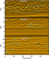 |
Fig. 2. Parabolic trajectories of dynamic fibrils. Panels a–c: contrast enhanced X-T maps from slit S1, S2, and S3, respectively. In each of these panels, the curves in cyan outline the fitted parabolas to the visually identified bright tracks. See Sect. 3.1 for details. |
3.2. Inspection of selected individual EUV dynamic fibrils
As mentioned earlier, the event movie reveals multiple bright structures that move up and down with time. To give some examples, through a series of snapshots in Fig. 3, we highlight how a blob-like moving bright feature creates a parabolic track in the X-T map. Figure 3a presents the X-T map from slit S1, which we recall is located in between two closed loops (see Fig. 1a). In all three highlighted cases (C1, C2, and C3), we find a small brightening with a size ≈0.5 Mm (i.e. only two to three EUI pixels) exhibiting up and down motions (see the snapshots in the panels on the right side of the figure). Cases C2 and C3 further highlight the repetitive nature of these phenomena. The other interesting aspect to note here is of the change in size of these features as they evolve with time. For example, in C1 we find that the size increases with time, whereas in C2 it remains almost constant, and in C3 it initially increases but then remains constant for the rest of the time.
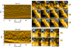 |
Fig. 3. Closer look at up and down motions. Panel a: contrast enhanced X-T map from Slit S1. The cyan boxes C1, C2, and C3 highlight the chosen tracks, whose snapshots are presented in the adjacent panels. In each of these panels, the brightening that creates the track is highlighted by an arrow wherein the track itself (from the X-T map) is shown in the greyscale inset panel. Cyan dots overlaid on each of these inset tracks are indicative of the time at which the EUI snapshots were taken. Panel b: contrast enhanced X-T map from Slit M3 along with two cases highlighted as C4 and C5. |
In another example, Fig. 3b shows the X-T map from M3 which is located on top of a moss region (see Fig. 1a). Interestingly, in the two highlighted cases from this map, that is C4 and C5, we find the brightenings to be of even smaller sizes (≊0.3 Mm) compared to those in Fig. 3a. Through these examples, we therefore confirm that the parabolic tracks in the X-T maps are indeed due to movements of blob-like bright EUV features.
3.3. Statistical properties of EUV dynamic fibrils
In this section we examine the statistical properties of these parabolic tracks. Of course, parameters such as speeds and lengths suffer from projection effects and, thus, the values that are quoted here are apparent ones. The results of this statistical analysis are summarised in Fig. 4. Different panels shown there outline the overall distributions (in grey) of deceleration (panel a), maximum length (panel b), maximum speed (panel c), and lifetime (panel d). We further segregated each of these parameters according to the slit type where the respective DFs were found. The histograms for the respective subsets of the S slits (green) and M slits (cyan) are overplotted in Fig. 4. We find that the median values of deceleration, maximum length, and maximum speed distributions of the DFs for S slits are higher than that for M slits (see Table 1). Lifetime distributions, however, have similar medians for both slit classes.
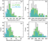 |
Fig. 4. Properties of DFs in EUV. Distributions of fitted parameters such as deceleration (panel a), maximum length (panel b), maximum speed (panel c), and lifetime (panel d). In each panel, the grey-shaded histogram presents the overall distribution of all analysed X-T map profiles (sample size n = 98) wherein the distributions derived only for S and M slits (n = 61 and 37, respectively) are shown in green and cyan colours, respectively. Further details are listed in Table 1. |
Statistical properties of EUV dynamic fibrils.
To check the statistical significance of the differences between the M slits in moss regions and the S slits close to sunspots, we performed a two-sided Kolmogorov–Smirnov (K-S) test between the samples from the two slit types. Basically, the K-S test compares the empirical cumulative distribution functions (ECDFs) of two samples and decides whether those two samples are drawn from the same parent population or not (Berger & Zhou 2014). The test statistic D is a measure of the maximum distance between two ECDFs, while the probability p endorses the null hypothesis that the two samples come from the same underlying population. As is often assumed, we reject the null hypothesis if p ≤ 0.05 and conclude that the two samples are inherently different from each other. The K-S test results of our samples, as summarised in the last rows of Table 1, validate the statistical significance of our earlier observation about the differences in the DF properties between S slits and M slits.
Lastly, we performed a brief comparison between the overall distributions of DFs that we have obtained in this study to that of the chromospheric observation of DFs by De Pontieu et al. (2007). By comparing the median values, we find that our deceleration median of 82 m s−2 is significantly lower than the value of 136 m s−2 given by De Pontieu et al. (2007) (we note that the deceleration distribution shown in their Letter is also quite broad). In the case of the lifetime, we obtain a higher median of 332 s as opposed to 250 s found by De Pontieu et al. (2007). Interestingly, the other two median values, that is of maximum length (1293 km) and maximum speed (14 km s−1), are comparable to the ones found by them. Further comparisons with the results by De Pontieu et al. (2007) are presented in Appendix A.
3.4. SDO view of EUV dynamic fibrils
Given the favourable (very small) angle between the SDO and Solar Orbiter, we also analysed the same region as seen by EUI, but using data from AIA, employing the same techniques as for the EUI data. We also added the magnetic field information acquired by HMI. Along with the EUI image, Fig. 5 presents co-temporal images from the co-aligned AIA 171 Å data (panel b) and the HMI line-of-sight magnetogram (panel c). As expected, the features in the AIA 171 Å image appear to be quite similar to those of EUI 174 Å image, while the magnetogram reveals a large-scale bipolar-type magnetic configuration of the host AR (NOAA12960). Furthermore, the overlaid slits on the magnetogram re-confirms our slit classification, that is to say the S slits touch the leading spot, whereas the M slits were placed away from it in plage-type areas that are expected below moss regions. The main reason to include SDO data here is to compare the visibility of the parabolic tracks of the DFs between EUI and AIA in the corresponding X-T maps. For illustration purposes, we chose two of the slits we already investigated with EUI, that is slit S1 which is located close to the spot and slit M3 which is located far away from that spot and lies on top of a moss region (cf. Figs. 5a−c). The AIA 6 s cadence dataset has regular data gaps (see Sect. 2), which somewhat distract our attention in those corresponding X-T maps (Figs. 5e, h), and therefore we also used the 12 s cadence (the usual AIA cadence) data and regenerated those X-T maps (Figs. 5f, i).
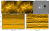 |
Fig. 5. Comparison between the EUI and AIA views of DFs. Panel a: snapshot from the EUI 174 Å time series, while a co-aligned, co-temporal AIA 171 Å image is shown in panel b and the HMI line of sight (LOS) magnetogram is displayed in panel c. All of these three panels have the slits from Fig. 1a overplotted on them. Panels d–f: slit-S1 X-T maps (contrast enhanced) derived using the EUI data, the AIA 171 Å 6 s image sequence, and the AIA 171 Å 12 s sequence, respectively. The same but for slit M3 are shown in panels g–i. The vertical lines in panels e and h represent the missing frames in that AIA dataset. |
By comparing the X-T maps of these slits between EUI and AIA (Figs. 5d−f and g, i), we found the following two main results: (1) there are significantly fewer parabolic tracks visible in AIA as compared to EUI, and (2) some of the AIA tracks are ambiguous and can only be identified in hindsight, that is only after seeing the corresponding EUI map. For example, the ambiguous signal in the AIA map (Fig. 5e) around T = (65, 85) min and X = (10, 13) Mm is clearly distinguishable in the corresponding EUI map (Fig. 5d). Considering the difference of a factor of ca. 2.5 in their spatial resolutions (cf. Sect. 2), it is not surprising that the DFs are much harder to detect, or in many cases not visible at all in AIA image sequences. The scenario that these small-scale features are not always detectable in AIA images is somewhat similar to the visibility of campfires in simultaneous EUI and AIA images as noted by Berghmans et al. (2021) and Mandal et al. (2021). This could also explain why Skogsrud et al. (2016) were not able to unambiguously detect counterparts of chromospheric DFs in AIA coronal data.
4. Discussion and summary
Using high-resolution, high-cadence EUV images from EUI 174 Å, we find bright blob-like features that repeatedly move up and down and leave parabolic tracks in X-T maps. The sizes of these blobs are between 0.3 Mm and 0.5 Mm. Other properties such as their speeds or lifetimes are very similar to chromospheric dynamic fibrils observed in Hα by De Pontieu et al. (2007). Hence, we conclude that these features are the EUV signatures of DFs. As mentioned in the Introduction, DFs are shock-driven chromospheric phenomena (Hansteen et al. 2006), and hence the brightenings that we find in EUI 174 Å images are probably the hot tips of those fibrils. Furthermore, the appearance of these bright parabolic tracks is strikingly similar to that of the ‘bright rims’ in IRIS 1400 Å images as noted by Skogsrud et al. (2016). Unfortunately, the transition region images from the coordinated IRIS observation have a negligible overlap with EUI, both in terms of spatial and temporal coverage, and thus we lack the lower atmospheric view of the EUV DF features we observed with EUI. Moreover, in the absence of such coordinated spectroscopic observations, we are unable to conclusively determine whether the EUV emission that we see in EUI comes from a coronal plasma (log T = 6) or from more of a slightly cooler transition region material (log T = 5.4). Future observations are needed to examine this further.
One of the interesting results we obtained from this study relates the properties of these DFs to their location of origin. For example, DFs that originate closer to a spot (e.g. S slits) are faster, longer, and decelerate more strongly than those that emerge from a moss region (e.g. M slits). Using chromospheric observations, De Pontieu et al. (2007) also found significant differences between DFs that come from a dense plage region (with a predominantly vertical magnetic field) and those that originate from a less dense plage region (with a more inclined field). These authors explained the observed differences in terms of a combination of shock waves and the local magnetic field topology. For instance, a vertical magnetic field guides 3-min oscillations, which possess less power compared to 5-min oscillations that are channelled along a more inclined field. As a result, DFs in inclined field regions have higher speeds (owing to higher driving power; Rouppe van der Voort & de la Cruz Rodríguez 2013) and lower deceleration (because only a component of gravity acts along the field lines; Hansteen et al. 2006). However, there is more to the story. As DFs are shock-driven phenomena, we expect a stronger shock (such as in inclined fields) to produce a greater deceleration (De Pontieu et al. 2007). In our study, we indeed find such signatures. For example, S-slit DFs show higher speeds than M slits and, at the same time, these S-slit DFs also suffer greater deceleration than M slits. This is also evident through the correlation analysis that we present in Appendix A. This further strengthens our explanation of the observed bright tracks as signatures of DFs.
Future studies using EUI data that accommodate DFs from a wide variety of magnetic regions will be helpful in further understanding such regional dependencies. A central element in such studies should be the combination of simultaneous observations of transition region and chromospheric plasma, requiring careful coordination between Earth-based facilities and Solar Orbiter. This will help in our understanding of the role of DFs in shaping the upper solar atmosphere in ARs.
To conclude, by analysing high-resolution, high-cadence EUV images from Solar Orbiter, we find bright dot-like features that move up and down with time (often repeatedly) and produce parabolic tracks in X-T diagrams. Their properties, such as speeds, lifetime, lengths, and deceleration, strongly suggest that these bright dots in the EUV images are a signature of the hot gas at or close to the tips of the chromospheric DFs.
Movie
Movie 1 associated with Fig. 1 (Fig1) Access Supplementary Material
Interface Region Imaging Spectograph; De Pontieu et al. (2014).
Swedish 1 m Solar Telescope; Scharmer et al. (2003).
This was coordinated as SOOP R-BOTH-HRES-HCAD nanoflares (Zouganelis et al. 2020; Berghmans et al. 2022).
We did not really observe the elongated fibrils in EUV, but rather only tips of them.
Acknowledgments
We thank the anonymous reviewer for the encouraging comments and helpful suggestions. Solar Orbiter is a space mission of international collaboration between ESA and NASA, operated by ESA. The EUI instrument was built by CSL, IAS, MPS, MSSL/UCL, PMOD/WRC, ROB, LCF/IO with funding from the Belgian Federal Science Policy Office (BELSPO); the Centre National d’Etudes Spatiales (CNES); the UK Space Agency (UKSA); the Bundesministerium für Wirtschaft und Energie (BMWi) through the Deutsches Zentrum für Luft- und Raumfahrt (DLR); and the Swiss Space Office (SSO). L.P.C. gratefully acknowledges funding by the European Union. Views and opinions expressed are however those of the author(s) only and do not necessarily reflect those of the European Union or the European Research Council (grant agreement No. 101039844). Neither the European Union nor the granting authority can be held responsible for them. The ROB team thanks the Belgian Federal Science Policy Office (BELSPO) for the provision of financial support in the framework of the PRODEX programme of the European Space Agency (ESA) under contract numbers 4000134474, 4000134088, and 4000136424. W.L. and M.C.M.C. acknowledge support from NASA’s SDO/AIA contract (NNG04EA00C) to LMSAL. AIA is an instrument on board the Solar Dynamics Observatory, a mission for NASA’s Living With a Star programme. W.L. is also supported by NASA grants 80NSSC21K1687 and 80NSSC22K0527. D.M.L. is grateful to the Science Technology and Facilities Council for the award of an Ernest Rutherford Fellowship (ST/R003246/1). S.P. acknowledges the funding by CNES through the MEDOC data and operations centre. This research has made use of NASA’s Astrophysics Data System. The authors would also like to acknowledge the Joint Science Operations Center (JSOC) for providing the AIA data download links.
References
- Berger, V. W., & Zhou, Y. 2014, Kolmogorov–Smirnov Test: Overview (American Cancer Society) [Google Scholar]
- Berger, T. E., De Pontieu, B., Fletcher, L., et al. 1999, Sol. Phys., 190, 409 [NASA ADS] [CrossRef] [Google Scholar]
- Berghmans, D., Auchère, F., Long, D. M., et al. 2021, A&A, 656, L4 [NASA ADS] [CrossRef] [EDP Sciences] [Google Scholar]
- Berghmans, D., Antolin, P., Auchère, F., et al. 2022, A&A, submitted [Google Scholar]
- De Pontieu, B., Erdélyi, R., & James, S. P. 2004, Nature, 430, 536 [Google Scholar]
- De Pontieu, B., Erdélyi, R., & De Moortel, I. 2005, ApJ, 624, L61 [Google Scholar]
- De Pontieu, B., Hansteen, V. H., Rouppe van der Voort, L., van Noort, M., & Carlsson, M. 2007, ApJ, 655, 624 [Google Scholar]
- De Pontieu, B., Title, A. M., Lemen, J. R., et al. 2014, Sol. Phys., 289, 2733 [Google Scholar]
- Hansteen, V. H., De Pontieu, B., Rouppe van der Voort, L., van Noort, M., & Carlsson, M. 2006, ApJ, 647, L73 [Google Scholar]
- Heggland, L., De Pontieu, B., & Hansteen, V. H. 2007, ApJ, 666, 1277 [Google Scholar]
- Krishna Prasad, S., Banerjee, D., Van Doorsselaere, T., & Singh, J. 2012, A&A, 546, A50 [NASA ADS] [CrossRef] [EDP Sciences] [Google Scholar]
- Lemen, J. R., Title, A. M., Akin, D. J., et al. 2012, Sol. Phys., 275, 17 [Google Scholar]
- Mampaey, B., Verbeeck, F., Stegen, K., et al. 2022, SolO/EUI Data Release 5.0 2022-04 (Royal Observatory of Belgium (ROB)), https://doi.org/10.24414/2qfw-tr95 [Google Scholar]
- Mandal, S., Peter, H., Chitta, L. P., et al. 2021, A&A, 656, L16 [NASA ADS] [CrossRef] [EDP Sciences] [Google Scholar]
- Mandal, S., Chitta, L. P., Antolin, P., et al. 2022, A&A, 666, L2 [NASA ADS] [CrossRef] [EDP Sciences] [Google Scholar]
- Müller, D., St. Cyr, O. C., Zouganelis, I., et al. 2020, A&A, 642, A1 [Google Scholar]
- Pesnell, W. D., Thompson, B. J., & Chamberlin, P. C. 2012, Sol. Phys., 275, 3 [Google Scholar]
- Rochus, P., Auchère, F., Berghmans, D., et al. 2020, A&A, 642, A8 [NASA ADS] [CrossRef] [EDP Sciences] [Google Scholar]
- Rouppe van der Voort, L., & de la Cruz Rodríguez, J. 2013, ApJ, 776, 56 [CrossRef] [Google Scholar]
- Rouppe van der Voort, L. H. M., De Pontieu, B., Hansteen, V. H., Carlsson, M., & van Noort, M. 2007, ApJ, 660, L169 [Google Scholar]
- Rutten, R. J. 2007, in The Physics of Chromospheric Plasmas, eds. P. Heinzel, I. Dorotovič, & R. J. Rutten, ASP Conf. Ser., 368, 27 [NASA ADS] [Google Scholar]
- Scharmer, G. B., Bjelksjo, K., Korhonen, T. K., Lindberg, B., & Petterson, B. 2003, in Innovative Telescopes and Instrumentation for Solar Astrophysics, eds. S. L. Keil, & S. V. Avakyan, SPIE Conf. Ser., 4853, 341 [NASA ADS] [CrossRef] [Google Scholar]
- Scherrer, P. H., Schou, J., Bush, R. I., et al. 2012, Sol. Phys., 275, 207 [Google Scholar]
- Skogsrud, H., Rouppe van der Voort, L., & De Pontieu, B. 2016, ApJ, 817, 124 [NASA ADS] [CrossRef] [Google Scholar]
- Zouganelis, I., De Groof, A., Walsh, A. P., et al. 2020, A&A, 642, A3 [NASA ADS] [CrossRef] [EDP Sciences] [Google Scholar]
Appendix A: Correlations and further comparisons
We analyse here the inter-relationships between various DF parameters by examining their scatter plots. From Fig. A.1a, we find a strong positive correlation between deceleration and maximum velocity. This means that a faster DF suffers more deceleration, while a DF that lives longer is subjected to less deceleration, as seen from the negative correlation in Fig. A.1b. In Fig. A.1d, we find that DFs that have higher speeds also have greater lengths. A positive correlation is further found between the maximum length and lifetime (Fig. A.1c), although with a significant spread for larger lengths. Lastly, no significant correlation is found either between maximum velocity and lifetime (Fig. A.1e) or among deceleration and maximum length (Fig. A.1f). All of these trends do match the findings of De Pontieu et al. (2007) who also performed a similar analysis but for chromospheric observations of DFs. As explained in De Pontieu et al. (2007), these correlations are basically a manifestation of the fact that DFs are a shock-driven phenomenon.
 |
Fig. A.1. Correlation analysis between different parameters of the fitted parabolas of EUV dynamic fibrils. Derived correlation coefficients (cc) for all three cases, i.e. for all slits, only S slits, and only M slits, are also printed on each panel. The green and blue circles represent DFs from the S slits and M slits, respectively. |
Appendix B: Multi-wavelength view
We present a multi-wavelength view of the studied AR NOAA12960 in Fig. B.1. Different panels in this figure display the outlook of that AR as seen through AIA and HMI channels. AIA channels such as the 94 Å, 131 Å, and 335 Å passbands, which are sensitive to emission from hotter plasma, highlight the presence of hot loops in the core of the AR. Furthermore, the footpoints of these hot loops seem to either coincide with or are located closer to the regions where M slits are positioned. These bright footpoint regions are typically referred to as moss regions (Berger et al. 1999).
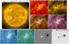 |
Fig. B.1. Multi-wavelength view of the AR NOAA12960. Panel a presents a full-disc 171 Å image from 2022 March 07, upon which the studied AR is outlined by the white rectangle. Zoomed-in views of that rectangular region from different AIA channels are shown in panels b−g, while images from HMI LOS and continuum channels are shown in panels i and j. The layout of the artificial slits overplotted on these panels is the same as in Fig. 1a. |
All Tables
All Figures
|
Fig. 1. Overview of the observed active region (AR). Panel a: sub-section of the HRIEUV full field of view from 2022 March 7. The boxes in various colours represent the artificial slits that we used to derive space-time (X-T) maps, some of which are shown in panels b−g. These X-T maps were contrast enhanced by performing a boxcar smooth subtraction along the space axis. The arrows drawn on every slit point to the increasing y-axis of the corresponding X-T maps. An animated version of this figure is available online. |
| In the text | |
|
Fig. 2. Parabolic trajectories of dynamic fibrils. Panels a–c: contrast enhanced X-T maps from slit S1, S2, and S3, respectively. In each of these panels, the curves in cyan outline the fitted parabolas to the visually identified bright tracks. See Sect. 3.1 for details. |
| In the text | |
|
Fig. 3. Closer look at up and down motions. Panel a: contrast enhanced X-T map from Slit S1. The cyan boxes C1, C2, and C3 highlight the chosen tracks, whose snapshots are presented in the adjacent panels. In each of these panels, the brightening that creates the track is highlighted by an arrow wherein the track itself (from the X-T map) is shown in the greyscale inset panel. Cyan dots overlaid on each of these inset tracks are indicative of the time at which the EUI snapshots were taken. Panel b: contrast enhanced X-T map from Slit M3 along with two cases highlighted as C4 and C5. |
| In the text | |
|
Fig. 4. Properties of DFs in EUV. Distributions of fitted parameters such as deceleration (panel a), maximum length (panel b), maximum speed (panel c), and lifetime (panel d). In each panel, the grey-shaded histogram presents the overall distribution of all analysed X-T map profiles (sample size n = 98) wherein the distributions derived only for S and M slits (n = 61 and 37, respectively) are shown in green and cyan colours, respectively. Further details are listed in Table 1. |
| In the text | |
|
Fig. 5. Comparison between the EUI and AIA views of DFs. Panel a: snapshot from the EUI 174 Å time series, while a co-aligned, co-temporal AIA 171 Å image is shown in panel b and the HMI line of sight (LOS) magnetogram is displayed in panel c. All of these three panels have the slits from Fig. 1a overplotted on them. Panels d–f: slit-S1 X-T maps (contrast enhanced) derived using the EUI data, the AIA 171 Å 6 s image sequence, and the AIA 171 Å 12 s sequence, respectively. The same but for slit M3 are shown in panels g–i. The vertical lines in panels e and h represent the missing frames in that AIA dataset. |
| In the text | |
|
Fig. A.1. Correlation analysis between different parameters of the fitted parabolas of EUV dynamic fibrils. Derived correlation coefficients (cc) for all three cases, i.e. for all slits, only S slits, and only M slits, are also printed on each panel. The green and blue circles represent DFs from the S slits and M slits, respectively. |
| In the text | |
|
Fig. B.1. Multi-wavelength view of the AR NOAA12960. Panel a presents a full-disc 171 Å image from 2022 March 07, upon which the studied AR is outlined by the white rectangle. Zoomed-in views of that rectangular region from different AIA channels are shown in panels b−g, while images from HMI LOS and continuum channels are shown in panels i and j. The layout of the artificial slits overplotted on these panels is the same as in Fig. 1a. |
| In the text | |
Current usage metrics show cumulative count of Article Views (full-text article views including HTML views, PDF and ePub downloads, according to the available data) and Abstracts Views on Vision4Press platform.
Data correspond to usage on the plateform after 2015. The current usage metrics is available 48-96 hours after online publication and is updated daily on week days.
Initial download of the metrics may take a while.