© The Authors 2023

1. Introduction

Peculiar (i.e., gravitational) velocities of galaxies are a robust probe for the search of dark matter on the large scales in the Universe. Their radial component can be computed in a basic way directly from galaxy distances. This method is immensely prone to a variety of Malmquist biases. In order to map the local dark matter distribution and to measure various cosmological parameters, modern cosmologists would rather use a full reconstruction in 3D of peculiar velocities. Such reconstructions are based on the Wiener filter algorithm, as well as forward modeling of the dataset and likelihood. Unfortunately, very few public releases of 3D peculiar velocity reconstructions are available to date, the largest one being the reconstruction from the redshift survey 2MASS by Lavaux & Hudson (2011). In this article, about 56 000 galaxy distances and 1000 supernovae distances from the CosmicFlows-4 (CF4) catalog are used to publicly release 3D reconstructions of the local Universe gravitational field.

The purpose of producing 3D reconstructions is not solely to create maps and cosmography of the nearby large-scale structures. The grids can also be used to test some cosmological hypothesis such as the general relativity model for gravity via the growth rate of large-scale structures (see, for example, Hudson & Turnbull 2012; Dupuy et al. 2019) and the homogeneity scale of the Universe via a test of the mean of all gravitational velocities enclosed in a sphere, the bulk flow. Both of these cosmology measurements are very sensitive to the number density of the catalogs and to the robustness and accuracy of the observed distance moduli.

For more than a decade, the measurement of distances of supernovae promises to the cosmologist more accuracy on distance moduli and more recently on bulk flow measurements than the classic galaxy distance relations. Already some literature exists that uses up to a few hundred supernovae distances to compute their peculiar velocities (without reconstruction) and to derive a measurement of the local Universe bulk flow. For more details, readers can refer to Dai et al. (2011), Turnbull et al. (2012), Feindt et al. (2013), Boruah et al. (2020), Mohayaee et al. (2021), and Peterson et al. (2022), for example. In this article we comparatively study galaxy and supernovae distances as probes of both the growth rate of structure fσ₈ and the bulk flow.

2. Data

The fourth release of the CosmicFlows catalog (Tully et al. 2022) provides about 56 000 measurements of galaxy distances and about 1000 supernovae distance moduli measurements. Such a composite catalog of distances delivers the raw material to compute radial peculiar velocities. Since the first CosmicFlows catalog, our peculiar velocity computational tools have evolved from direct analysis of Malmquist-biased radial peculiar velocities (CF1 1600 galaxies), to the Wiener filter linear 3D-reconstructed dataset (CF2: 8000 galaxies), which allowed for some modern cosmography of our local Universe to be built (Courtois et al. 2013), to a forward modeling iterative procedure for the third, much larger dataset (CF3: 18 000 galaxies). CF3 reached greater distances in the southern terrestrial hemisphere and was used to discover distant features such as the Cold Spot Repeller (Courtois et al. 2017) and the Vela Supercluster (Courtois et al. 2019). The current CF4 dataset is three times larger in terms of the number of galaxies than CF3 and it is doubling its reach in the northern hemisphere.

3. Growth rate measurement from radial peculiar velocities

In this Letter, we use a velocity statistical indicator, noted ψ₁, introduced by Gorski et al. (1989). This indicator only depends on radial peculiar velocities, and ψ₁ is defined as follows:

$$\begin{array}{c}\hfill {\psi }_1(r)=\frac{\sum {\mathit{u}}_A·{\mathit{u}}_B}{\sum {({\widehat{\mathit{r}}}_A·{\widehat{\mathit{r}}}_B)}^2}=\frac{\sum u_A{u}_{B}cos{\theta }_{\mathit{AB}}}{\sum {cos}^2{\theta }_{\mathit{AB}}}.\end{array}$$(1)

Dupuy et al. (2019), using the direct radial peculiar velocities of the CF3 dataset, found fσ₈ = 0.43(±0.03)_obs(±0.11)_{cos. var.} out to z = 0.05.

Figure 1 shows the computation of the estimator Ψ₁ using the radial peculiar velocities of the 1008 supernovae in CF4 (in green), and of the 36 000 galaxy groups in CF4 (in blue) and the full 56 000 individual galaxies (in red). It appears clearly that the small number of supernovae per bin of pairwise separation is too small for pairwise separations smaller than 20–30 $h_{100}^{-1}$ Mpc. w of the CF4 catalog provide results that concord for the two samples across the whole range of pairwise separations.

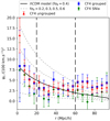Fig. 1. Estimator to compute the growth rate of structures using 1008 supernovae (in green), 36 000 galaxy groups (in blue), and 56 000 individual galaxy distances (in red). Computation was carried out as in Dupuy et al. (2019). The distance r is the pairwise separation bin in $h_{100}^{-1}$ Mpc between radial peculiar velocities in the datasets. Error bars represent the observational errors of the distance moduli (no cosmic variance is considered in this plot). The number density of data per bin of pairwise separation is of crucial importance in order to assess the result. The current supernovae sample is too sparse for separations smaller than 20–30 $h_{100}^{-1}$ Mpc.

This procedure has provided the following for the supernovae: fσ₈  =  0.28(±0.09)_obs for the pairwise separation range 20–30 $h_{100}^{-1}$ Mpc, fσ₈  =  0.31(±0.06)_obs for the range 20–60 $h_{100}^{-1}$ Mpc, and fσ₈  =  0.30(±0.06)_obs for the range 20–80 $h_{100}^{-1}$ Mpc. We obtain fσ₈  =  0.32(±0.07)_obs for the grouped CF4 and fσ₈  =  0.36(±0.06)_obs for the individual galaxies in CF4, with both being for the pairwise separation range 20–60 $h_{100}^{-1}$ Mpc. All errors were computed using the observational errors of the distance moduli. Cosmic variance is much larger and in Dupuy et al. (2019) we determined that it would account for about ±0.11 in the volume of the Universe covered by CosmicFlows catalogs. This value should be compared to the y axis of Fig. 7 in that paper. Here, we recomputed the growth rate with the same methodology applied to CF4 radial peculiar velocities, and error bars represent observational errors only. However, the error bars do include the number density in each bin. The two-point velocity statistic considered here allows for the underlying cosmology from a homogeneous and spherical universe to be computed. As tested and explained in Dupuy et al. (2019), the unique geometry of the CF3 and CF4 catalogs would impact the findings about the underlying cosmology for pairwise separation distances larger than 60 Mpc h⁻¹.

4. 3D gravitational velocity field and bulk flow

In order to compute a 3D reconstruction of the CF4 catalog, we used an iterative forward modeling procedure with a Hamiltonian Monte-Carlo (HMC) algorithm that explores the values of some free parameters (i.e., Ω_m, bias, scatter component of the nonlinearity in the velocity field solution σ_NL, among others). This procedure is an extension of the procedure used for the CF3 catalog described in Graziani et al. (2019) and briefly hereafter.

To obtain the linear particular velocity field, the following linearized continuity equation was used:

$$\begin{array}{c}\hfill \frac{\partial \delta }{\partial t}+\frac{1}{a}{\mathbf{\nabla }}_{\chi }.\mathit{v}=0,\end{array}$$(2)

where the over-density field is

$$\begin{array}{c}\hfill \delta (\mathit{x},t)=D_{+}(t){\delta }_0(\mathit{x}),\end{array}$$(3)

where D₊(t) is the linear growth factor. Indeed, the linear approximation carried out in this article gives the linear temporal evolution of the over-density field. The continuity equation then becomes the following:

$$\begin{array}{c}\hfill {\mathbf{\nabla }}_{\chi }.\mathit{v}=-\dot{D}{\delta }_0=-\frac{\mathrm{d}ln(D)}{\mathrm{d}ln(a)}\dot{a}\delta =-\dot{a}f\delta ,\end{array}$$(4)

where $f=\frac{\mathrm{d}ln(D)}{\mathrm{d}ln(a)}$ is the growth rate of large scale structures. The power spectrum P(k) is the function that characterizes the amplitude of the perturbations in Fourier space, as a function of the scale of these disturbances. The velocity power spectrum corresponds to the over-density power spectrum times $\frac{1}{k^2}$. This means that the peculiar velocity field is less affected by small-scale changes and is more strongly correlated at large scales.

The Bayesian model used here is an adaptation of a model developed by Lavaux (2016). Two observations are used for each galaxy in the catalog: the distance modulus μ and the observed velocity v_CMB = cz_obs.

The conditional probability of the distance modulus knowing the parameters is the following:

$$\begin{array}{c}\hfill P(\mu |d)=N(5log(\frac{h_{\mathrm{eff}}d}{10\mathrm{pc}}),{\sigma }_{\mu }^2;\mu ).\end{array}$$(5)

The μ probability is a Gaussian centered around $5log(\frac{h_{\mathrm{eff}}d}{10\mathrm{pc}})$ and with standard deviation σ_μ, which corresponds to the error of the measurement of the distance modulus. The parameter h_eff is quite important in the model. It traces zero-point intercalibration problems between different distance methodologies used in the CosmicFlows catalogs. The relationship between the distance modulus and the luminosity distance is valid up to a constant. This constant is the zero point of the law that indicates the distance and which must be calibrated. This calibration is not independent of the value of H₀ and its value could influence the reconstruction performed. The conditional probability of the observed redshift knowing the parameters is given by the following:

$$\begin{array}{c}\hfill P(z|\mathit{v},d,{\sigma }_{\mathrm{NL}},\mathit{r})=N(\mathit{v}.\mathit{r},{\sigma }_{\mathit{cz}}^2{(1+\overline{z})}^{-2}+{\sigma }_{\mathrm{NL}}^2,v_{\mathrm{pec}}^{\mathrm{r}}),\end{array}$$(6)

where ${\mathit{v}}_{\mathrm{pec}}^{\mathrm{r}}$ is the radial peculiar velocity. It is a Gaussian law centered around the reconstructed velocity for each point of the grid, with its standard deviation being a combination between the typical error of the observed redshift σ_cz and a σ_NL parameter. The purpose of the latter is to absorb the nonlinearities of the observed velocities.

The likelihood function was then constructed as the product of the conditional probabilities in Eqs. (5) and (6). Priors are functions that assign a probability to each state in the parameter space. These functions guide the sampling toward high probability parameter values and, when chosen carefully, accelerate the convergence of the sampling.

In the case of the model used here, the parameters for which a prior must be chosen are h_eff, σ_NL, {d_i}, and v. The particular velocities are known a priori thanks to the power spectrum of the chosen cosmological paradigm (here LCDM from Planck Collaboration XIII 2016), which makes it possible to define an a priori over-density field:

$$\begin{array}{c}\hfill P(\delta (\mathit{k})|\mathrm{\Lambda }\mathrm{CDM})={\displaystyle \prod _{\mathit{k}}N(0,P(\mathit{k})).}\end{array}$$

This prior for the over-density field allowed us to derive the prior for the peculiar velocity field in Fourier space using linear perturbation theory. This realization of the velocity field was then constrained by the observational data using the Wiener filter constrained realizations as described, for example, in Doumler et al. (2013). This work provides a brief overview on how to reconstruct the 3D peculiar velocity field.

The reconstruction codes we have used are continuously improved by our team and thoroughly tested. The one used for this article already shows limitations: namely in the time needed to compute reconstructions of large datasets such as CF4. Thus we are also testing newer reconstruction methods that will allow us to analyze the upcoming datasets of WALLABY, DESI, and 4HS peculiar velocity surveys, which will be an order of magnitude larger than CF4.

Since CF4 is made up of several surveys, an additional step is needed to prevent Malmquist biases and zero-point calibration errors. This prior is an arbitrarily chosen function that models the expected behavior of the distance distribution. We followed Lavaux (2016) by fitting a function with three parameters, a, b, and c, to the distribution of redshifts. Figure A.1 shows that the catalog contains two classes of supernovae and also two classes of galaxy distances: a class of data with high accuracy (labeled type 0) with errors for distance moduli being smaller than 0.5 mag (in blue) and a medium accuracy class of data (labeled type 1) with errors for distance moduli being larger or equal to 0.5 mag (in green).

In this article all computations have been carried out with the ΛCDM cosmological model with initial values of Ω_m = 0.3, H₀ = 74.6 km s⁻¹ Mpc⁻¹ (the nominal value for the CF4 catalog given in Tully et al. 2022), and a limitation of k_max = 0.1 for the smallest phases reconstructed in Fourier space. In order to reach a stable convergence on the parameters, the computation requires approximately 3000 HMC steps for both the supernovae subsample and the full CF4 dataset. However, we have gone well beyond the convergence and computed about 10 000 HMC steps in order to subsequently derive mean solutions that are less correlated and more statistically robust. The resulting over-density δ and gravitational velocity fields were averaged (after removing the burning steps of the HMC). The resulting velocity fields are presented in this article for resolutions of 64³ up to z = 0.08 for the CF4 dataset and its supernovae subsample. This yields about 8 h⁻¹ Mpc per voxel. A voxel is the cubic volume in a 3D density grid. Its size depends on the resolution of the grid. The nonlinear component of the velocity field, which is a free parameter of the HMC exploration, has a mean value of ${\sigma }_{\mathrm{NL}}^{\mathrm{CF}4\mathrm{gp}}=170$ km s⁻¹, ${\sigma }_{\mathrm{NL}}^{\mathrm{CF}4}=300$ km s⁻¹, and ${\sigma }_{\mathrm{NL}}^{\mathrm{supernovae}}=250$ km s⁻¹.

The exploration of the 10 000 reconstructions has led to the conclusion that the distances delivered by the CF4 catalog are compatible with a Hubble constant of H₀ = 74.5 ± 0.1 (grouped CF4), H₀ = 75.0 ± 0.35 (ungrouped CF4), and H₀ = 75.5 ± 0.95 (CF4 supernovae subsample).

Figure 2 shows the reconstructed 3D density δ_m and velocity v_m gravitational fields for the three datasets. It is important that the same large-scale structures be found within the first 100 $h_{100}^{-1}$ Mpc around the observer with all datasets. Those are the first published 3D reconstructions of CF4. The largest structure known in the local Universe, the Sloan great wall, is clearly seen at SGY of 250 $h_{100}^{-1}$ Mpc and extends over more than 400 $h_{100}^{-1}$ Mpc along the SGX coordinates. One of the improvements compared to previous CosmicFlows reconstructions is that now we also deliver the standard deviation of the peculiar velocity field over the HMC forward modeling process. In Fig. 2, the right panels show this standard deviation in km s⁻¹. Nearby, in a radius of about 200 $h_{100}^{-1}$ Mpc around the observer located at (SGX = 0, SGY = 0), the reconstruction we publish is robust at the level of 50–80 km s⁻¹.

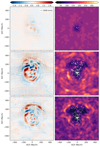Fig. 2. Over-density δ and velocity gravitational fields 3D reconstructions of the CF4 supernovae sample (top row), full galaxy sample (ungrouped and grouped in the middle and bottom row, respectively), projected onto the supergalactic coordinate SGX–SGY plane (left column). Velocity field standard deviation in km s−1 over the 10 000 HMC steps of the respective computations of the left panels (right column). The white dots are the CF4 data in a slice of ±2 $h_{100}^{-1}$ Mpc on the SGZ axis. In the nearby Universe close to the observer, located at the center of the box, all datasets reconstruct the same large-scale structures, with a robustness in the peculiar velocity field of about 50 km s−1. The Sloan great wall appears at SGY 250 $h_{100}^{-1}$ Mpc as a major feature of our local Universe.

From the 3D velocity field, we computed a basic estimation of the bulk flow as the mean of the gravitational velocities, which are at rest in the cosmic microwave background, inside a sphere of radius R. The errors of the bulk flow were computed from the standard deviation of the peculiar velocity field obtained through the variations of each of the realizations during the HMC forward modeling process.

Figure 3 shows the amplitude of the bulk flow (bottom panel) and of its three components along the supergalactic X, Y, and Z axis (top panel), as a function of the radius of the sphere centered at the observer location. The error bars for the 3D reconstruction were computed from the standard deviations on the 10 000 HMC realizations. At large radii, where the prior model of an homogeneous universe dominates over the observational data, the bulk flow vanishes. Both the supernovae and the full CF4 sample concord and detect the large nearby attractors located within [100–150] $h_{100}^{-1}$ Mpc from the observer: Centaurus, Great Attractor, and Coma. Inside 150 $h_{100}^{-1}$ Mpc, the CF4 bulk flow is (272 ± 105) km s⁻¹, which is in complete accordance with our previous measurement of (239 ± 38) km s⁻¹ using the CF2 dataset (Hoffman et al. 2015). Using 1008 supernovae, we find a bulk flow of 227 ± 131 km s⁻¹ at 100 $h_{100}^{-1}$ Mpc (see Table 1), which is in agreement with Turnbull et al. (2012) using 245 supernovae peculiar velocities who measured a bulk flow of 249 ± 76 km s⁻¹ out to 110 $h_{100}^{-1}$ Mpc.

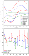Fig. 3. Bulk flow components along the supergalactic X, Y, and Z axis (top panel) and its norm (bottom panel), as a function of the radius R of a sphere centered at the observer location. The velocities are in km s−1 at rest in the cosmic microwave background. The error bars for the 3D reconstruction were computed from the standard deviations of 10 000 HMC realizations. The reader is reminded that the supernovae dataset only extends out to 100 $h_{100}^{-1}$ Mpc and it is too sparse to fully recover the velocity field.

Further out from the observer, the impact of the Sloan great wall is clearly seen in Fig. 3 with a strong pull along the SGY direction within the range of distances, [250–300] $h_{100}^{-1}$ Mpc, contributing to a bulk flow of 230 km s⁻¹ at the largest distance tested, 300 $h_{100}^{-1}$ Mpc. This value is in strong disagreement with Kashlinsky et al. (2010), who found – using X-ray emission of clusters of galaxies – a bulk flow of about 1000 ± 300 km s⁻¹ that is constant across the range [175–525] $h_{100}^{-1}$ Mpc.

5. Conclusions

This analysis of the CF4 catalog provides an estimated growth rate of structures of fσ₈ = 0.36(±0.05)_obs, while the similar previous measurement with CF3 was fσ₈ = 0.43(±0.03)_obs(±0.11)_{cos. var.}. At the largest distance of the observational data, we obtain a bulk flow measurement of 230 ± 136 km s⁻¹ at a distance of 300 $h_{100}^{-1}$ Mpc, which is pointing in the direction of the Sloan great wall. Another conclusion is that, although the current supernovae sample is very small, it is dense enough for an acceptable local fσ₈ measurement. However, the supernovae dataset only extends out to 100 $h_{100}^{-1}$ Mpc and is too sparse to fully recover the velocity field and, as a consequence, it cannot be used as a probe of the bulk flow yet.

From the tight variation around ΛCDM values of the free parameters explored by the convergence of the HMC forward modeling and in light of the values obtained for two cosmology-related parameters – namely the growth rate and bulk flow – we conclude that this analysis of the local Universe using peculiar velocities is compatible with a ΛCDM cosmology.

The density and velocity gravitational fields’ 3D reconstructions on grids will be publicly available¹. We also go one step further, compared to our previous CosmicFlows analysis, by delivering the accompanying 3D standard deviation grids of the reconstructed gravitational fields in order for future users to better estimate their analysis robustness.

Acknowledgments

HC is grateful to the Institut Universitaire de France for its huge support which enabled this research. HC, DG and FR acknowledge support from the CNES. AD is supported by a KIAS Individual Grant (PG087201) at Korea Institute for Advanced Study.

References

Appendix A: Additional figure

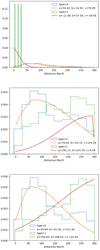Fig. A.1. Gaussian fitting of the normalized initial distance distribution of the CF4 supernovae sample (top panel), ungrouped CF4 catalog (middle panel), and grouped CF4 catalog (bottom panel). The priors were fit according to the precision of the distance moduli: less than 0.5 mag errors were modeled as class 0, and ≥0.5mag errors are in class 1.

All Tables

All Figures

Fig. 1. Estimator to compute the growth rate of structures using 1008 supernovae (in green), 36 000 galaxy groups (in blue), and 56 000 individual galaxy distances (in red). Computation was carried out as in Dupuy et al. (2019). The distance r is the pairwise separation bin in $h_{100}^{-1}$ Mpc between radial peculiar velocities in the datasets. Error bars represent the observational errors of the distance moduli (no cosmic variance is considered in this plot). The number density of data per bin of pairwise separation is of crucial importance in order to assess the result. The current supernovae sample is too sparse for separations smaller than 20–30 $h_{100}^{-1}$ Mpc.

In the text

Fig. 2. Over-density δ and velocity gravitational fields 3D reconstructions of the CF4 supernovae sample (top row), full galaxy sample (ungrouped and grouped in the middle and bottom row, respectively), projected onto the supergalactic coordinate SGX–SGY plane (left column). Velocity field standard deviation in km s−1 over the 10 000 HMC steps of the respective computations of the left panels (right column). The white dots are the CF4 data in a slice of ±2 $h_{100}^{-1}$ Mpc on the SGZ axis. In the nearby Universe close to the observer, located at the center of the box, all datasets reconstruct the same large-scale structures, with a robustness in the peculiar velocity field of about 50 km s−1. The Sloan great wall appears at SGY 250 $h_{100}^{-1}$ Mpc as a major feature of our local Universe.

In the text

Fig. 3. Bulk flow components along the supergalactic X, Y, and Z axis (top panel) and its norm (bottom panel), as a function of the radius R of a sphere centered at the observer location. The velocities are in km s−1 at rest in the cosmic microwave background. The error bars for the 3D reconstruction were computed from the standard deviations of 10 000 HMC realizations. The reader is reminded that the supernovae dataset only extends out to 100 $h_{100}^{-1}$ Mpc and it is too sparse to fully recover the velocity field.

In the text

	Fig. A.1. Gaussian fitting of the normalized initial distance distribution of the CF4 supernovae sample (top panel), ungrouped CF4 catalog (middle panel), and grouped CF4 catalog (bottom panel). The priors were fit according to the precision of the distance moduli: less than 0.5 mag errors were modeled as class 0, and ≥0.5mag errors are in class 1.
In the text

References

- Boruah, S. S., Hudson, M. J., & Lavaux, G. 2020, MNRAS, 498, 2703 [Google Scholar]
- Courtois, H. M., Pomarède, D., Tully, R. B., Hoffman, Y., & Courtois, D. 2013, AJ, 146, 69 [NASA ADS] [CrossRef] [Google Scholar]
- Courtois, H. M., Tully, R. B., Hoffman, Y., et al. 2017, ApJ, 847, L6 [NASA ADS] [CrossRef] [Google Scholar]
- Courtois, H. M., Kraan-Korteweg, R. C., Dupuy, A., Graziani, R., & Libeskind, N. I. 2019, MNRAS, 490, L57 [NASA ADS] [CrossRef] [Google Scholar]
- Dai, D.-C., Kinney, W. H., & Stojkovic, D. 2011, J. Cosmol. Astropart. Phys., 2011, 015 [CrossRef] [Google Scholar]
- Doumler, T., Hoffman, Y., Courtois, H., & Gottlöber, S. 2013, MNRAS, 430, 888 [NASA ADS] [CrossRef] [Google Scholar]
- Dupuy, A., Courtois, H. M., & Kubik, B. 2019, MNRAS, 486, 440 [NASA ADS] [CrossRef] [Google Scholar]
- Feindt, U., Kerschhaggl, M., Kowalski, M., et al. 2013, A&A, 560, A90 [NASA ADS] [CrossRef] [EDP Sciences] [Google Scholar]
- Gorski, K. M., Davis, M., Strauss, M. A., White, S. D. M., & Yahil, A. 1989, ApJ, 344, 1 [NASA ADS] [CrossRef] [Google Scholar]
- Graziani, R., Courtois, H. M., Lavaux, G., et al. 2019, MNRAS, 488, 5438 [NASA ADS] [CrossRef] [Google Scholar]
- Hoffman, Y., Courtois, H. M., & Tully, R. B. 2015, MNRAS, 449, 4494 [Google Scholar]
- Hudson, M. J., & Turnbull, S. J. 2012, ApJ, 751, L30 [NASA ADS] [CrossRef] [Google Scholar]
- Kashlinsky, A., Atrio-Barandela, F., Ebeling, H., Edge, A., & Kocevski, D. 2010, ApJ, 712, L81 [Google Scholar]
- Lavaux, G. 2016, MNRAS, 457, 172 [NASA ADS] [CrossRef] [Google Scholar]
- Lavaux, G., & Hudson, M. J. 2011, MNRAS, 416, 2840 [Google Scholar]
- Mohayaee, R., Rameez, M., & Sarkar, S. 2021, Eur. Phys. J. Special Topics, 230, 2067 [NASA ADS] [CrossRef] [Google Scholar]
- Peterson, E. R., Kenworthy, W. D., Scolnic, D., et al. 2022, ApJ, 938, 112 [NASA ADS] [CrossRef] [Google Scholar]
- Planck Collaboration XIII 2016, A&A, 594, A13 [NASA ADS] [CrossRef] [EDP Sciences] [Google Scholar]
- Tully, R. B., Kourkchi, E., Courtois, H. M., et al. 2022, ApJ, submitted [arXiv:2209.11238] [Google Scholar]
- Turnbull, S. J., Hudson, M. J., Feldman, H. A., et al. 2012, MNRAS, 420, 447 [Google Scholar]