| Issue |
A&A
Volume 670, February 2023
|
|
|---|---|---|
| Article Number | A151 | |
| Number of page(s) | 16 | |
| Section | Galactic structure, stellar clusters and populations | |
| DOI | https://doi.org/10.1051/0004-6361/202244919 | |
| Published online | 17 February 2023 | |
The most massive stars in very young star clusters with a limited mass: Evidence favours significant self-regulation in the star formation processes
1
School of Astronomy and Space Science, Nanjing University, Nanjing 210093, PR China
e-mail: yan@nju.edu.cn
2
Key Laboratory of Modern Astronomy and Astrophysics (Nanjing University), Ministry of Education, Nanjing 210093, PR China
3
European Southern Observatory, Karl-Schwarzschild-Straße 2, 85748 Garching bei München, Germany
e-mail: tereza.jerabkova@eso.org
4
Helmholtz-Institut für Strahlen- und Kernphysik (HISKP), Universität Bonn, Nussallee 14–16, 53115 Bonn, Germany
e-mail: pkroupa@uni-bonn.de
5
Charles University in Prague, Faculty of Mathematics and Physics, Astronomical Institute, V Holešovičkách 2, 180 00 Praha 8, Czech Republic
Received:
8
September
2022
Accepted:
16
November
2022
The stellar initial mass function (IMF) is commonly interpreted to be a scale-invariant probability density distribution function (PDF) such that many small clusters yield the same IMF as one massive cluster of the same combined number of stars. Observations of the galaxy-wide IMF challenge this as dwarf galaxies do not form as many massive stars as expected. This indicates a highly self-regulated star formation process in which stellar masses are not stochastically sampled from the IMF and are instead related to the environment of star formation. Here, we study the nature of star formation using the relation between the most massive star born in a star cluster and its parental stellar cluster mass (the mmax − Mecl relation). This relation has been argued to be a statistical effect if stars are sampled randomly from the IMF. By comparing the tightness of the observed mmax − Mecl distribution with synthetic star clusters with stochastically sampled stellar masses, we find that the expected dispersion of the mock observations is much larger than the observed dispersion. Assuming that mmax and Mecl uncertainties from the literature are correct, our test rejects the hypothesis that the IMF is a PDF at a more than 4.5σ confidence level. Alternatively, we provide a deterministic stellar mass sampling tool that reproduces the observed mmax − Mecl distribution and compares well with the luminosities of star-forming molecular clumps. In addition, we find that there is a significant flattening of the mmax − Mecl relation near mmax = 13 M⊙. This may suggest strong feedback of stars more massive than about 13 M⊙, and/or that the ejections of the most massive stars from young clusters in the mass range 63 to 400 M⊙ are likely important physical processes in forming clusters.
Key words: stars: formation / stars: luminosity function, mass function / stars: statistics / open clusters and associations: general / galaxies: stellar content / methods: statistical
© The Authors 2023
 Open Access article, published by EDP Sciences, under the terms of the Creative Commons Attribution License (https://creativecommons.org/licenses/by/4.0), which permits unrestricted use, distribution, and reproduction in any medium, provided the original work is properly cited.
This article is published in open access under the Subscribe-to-Open model. Subscribe to A&A to support open access publication.
1. Introduction
The nature of the discreteness of the stellar initial mass distribution function (IMF) is important to consider (Applebaum et al. 2020; Smith 2021). Different methods to sample stellar masses from an IMF have been discussed (Sormani et al. 2017; Hu et al. 2017; Hirai et al. 2021) and applied in an increasing number of recent studies of stellar systems with a low mass or a low star formation rate (SFR) and a high resolution of time or mass, starting to account for the evolution of individual massive stars (Gatto et al. 2017; Emerick et al. 2019; Lahén et al. 2020; Gutcke et al. 2021; Hislop et al. 2022) and even low-mass stars down to 0.08 M⊙ (where M⊙ is the solar mass; Hu 2019; Smith et al. 2021; Lahén et al. 2022).
It has been long known that simple stellar population (SSP) modelling codes, such as GALEV (Anders & Fritze-v. Alvensleben 2003) and Starburst99 (Vázquez & Leitherer 2005), neglect the discrete nature of the stellar mass distribution. This introduces a systematic offset in the colour prediction for star clusters that are young (< 80 Myr) or have a low mass (< 106 M⊙; Cerviño & Luridiana 2004). Ignoring the discreteness of the IMF significantly affects the inferred properties of low-mass systems, such as the evolution of star clusters (Wang & Jerabkova 2021; Dinnbier et al. 2022) or determinations of their age and mass, introducing errors in cluster ages as high as an order of magnitude (Piskunov et al. 2009).
In dynamical simulations of galaxies, an ensemble of stars – referred to as a ‘star particle’ – with a mass resolution of for example 105 M⊙ is often tracked instead of individual stars. In the simulation of single dwarf galaxies (and in recent years, the cosmological galaxy simulations, which are pushing to higher and higher resolutions to study ultra-faint galaxies), the number of stars in a galaxy or star particle becomes low enough that the integrated number of stars between two mass limits of the IMF (given by the considered time step and the stellar mass–lifetime relation, cf. Yan et al. 2019 their Fig. 3) can be less than one. If the IMF is still given as a continuous function, a fraction of a supernova explosion would result in such time steps in a simulation (Revaz et al. 2016; Applebaum et al. 2020). It has been demonstrated that a more realistic description of a stellar population, with a list of sampled stellar masses, alters the property and the evolution of the simulated galaxy compared to a model with a continuous energy injection due to the smooth IMF assumption, affecting the galactic SFR (Su et al. 2018), the strength of photoionisation (Smith 2021), galactic outflow (Smith et al. 2021), and chemical composition (Carigi & Hernandez 2008).
However, an important question that has not been resolved is how to sample stellar masses from a given IMF. There are two extreme sampling methods: stochastic sampling (also known as random sampling) and optimal sampling. Stochastic sampling is based on the hypothesis that the formation of every single star is purely an independent event and the mass of the star is randomly sampled from a probability density distribution function (PDF); that is, the IMF is considered to be a PDF. On the other end, optimal sampling (Kroupa et al. 2013; Schulz et al. 2015) assumes that the formation of all the stars (or at least all the massive stars that can be more accurately counted) in a star cluster is strongly correlated because of self-regulation of the star formation process, and therefore that a deterministic relationship exists between the mass of a star cluster and the mass of every single (massive) star within that cluster.
Theoretically, the sampling method relates to the fundamental astrophysics knowledge of the formation process of massive stars, which is not well understood. If the star formation process is sensitive to the initial conditions of the molecular cloud, such as angular momentum, shock wave behaviour, and so on, then stochastic sampling will be a reasonable approximation. For example, in the competitive accretion model (Bonnell et al. 1997, 1998, 2001), the stellar mass is gathered during the star-formation process as the parent cloud is randomly influenced by dynamical interactions. On the other hand, it is also possible that massive star formation is strongly regulated by feedback processes such as winds, outflows, radiation, accretion shocks, and the magnetic field of the parent cloud (Shu et al. 1987; Silk 1995; Adams & Fatuzzo 1996; Li & Nakamura 2006; Crutcher & Troland 2007) such that the random initial conditions are not as important. The stars formed in a single star formation event may then follow the IMF tightly with much more certainty than the random scenario. Another possibility is that a significant self-regulated formation of star clusters does not even require feedback regulation, as nature can automatically form the power-law distribution through scale-invariance, self-similarity, and iterative processes. For example, in preferential attachment phenomena and diffusion-limited aggregation, a large number of random processes (instead of a single stochastic event) determine the outcome, which becomes highly deterministic. The state-of-art star cluster formation simulation, STARFORGE, appears to support this view (Guszejnov et al. 2022). Despite the chaotic and complex physical processes involved, the simulated maximum stellar masses in embedded star clusters1 presented by these latter authors seem to have too little scatter to be explained by stochastic sampling schemes and to show strong evidence of a correlation between the embedded star cluster mass and the mass of the most massive star (mmax − Mecl relation), which is consistent with optimal sampling.
A variety of observational clues suggesting a highly self-regulated star formation process instead of a statistical process were discussed by Kroupa (2015, Table 1 therein). A non-trivial correlation between mmax and Mecl is evident through empirical (Larson 1982, 2003), analytical (Elmegreen 2000), and numerical (Bonnell et al. 2003, 2004) studies. The tight relation is particularly emphasised by Weidner & Kroupa (2006), Weidner et al. (2010, 2013) and reinforced by Stephens et al. (2017) and Yan et al. (2017), suggesting a significant self-regulation in the star formation process. André et al. (2016) find that stars form in molecular-cloud overdensities from inflows along filaments with remarkably similar cross sections of about 0.1 pc in radius, suggesting that star formation may be governed by relatively simple universal laws. A direct comparison of the fibre networks in B213 in Taurus and the NGC 1333 region in Perseus suggests that the differences between the classically distinguished isolated and clustered star-formation scenarios might originate from the same type of fibre with different densities. Furthermore, interactions between fibres may be responsible for the formation of massive cores and stars (Hacar et al. 2017). Recent observations also reveal regions with numerous low-mass correlated star formation events (CSFEs, also known as embedded clusters) that do not possess any massive star. For example, the whole southern part of the Orion southern cloud, L1641, despite being the origin of the formation of thousands of stars, has not formed a single massive star (see e.g. Hsu et al. 2012, 2013; Megeath et al. 2016). This is consistent with the mmax − Mecl relation because the southern cloud has only been forming low-mass embedded clusters. These CSFEs have radii consistent with the filament cross sections (Marks & Kroupa 2012). In addition, González-Lópezlira et al. (2012) and Pflamm-Altenburg et al. (2013) study the cluster mass distribution at different galactic radii of the flocculent galaxy M 33 and conclude that their mass is not randomly distributed.
Motivated by the above observations, Kroupa et al. (2013, their Sect. 2.2) suggest that the optimal sampling hypothesis better describes nature. In particular, optimal sampling is crucial to understand the top-light IMF (lack of massive stars compared to canonical IMF) of dwarf galaxies, which is evident from their Hα-to-FUV luminosity ratio (Pflamm-Altenburg et al. 2007, 2009; Lee et al. 2009), the mass–metallicity relation of galaxies (Köppen et al. 2007), and their α-element enhancement in comparison to the Milky Way (MW, Recchi et al. 2009; Yan et al. 2020; Minelli et al. 2021; Mucciarelli et al. 2021). With optimal sampling, the dwarf galaxies with a low SFR do not form massive stars (Yan et al. 2017, their Fig. 7). This is not the case in stochastic sampling, where the formation of massive stars happens randomly throughout the formation history of a galaxy such that the ratio between all the low-mass and massive stars ever formed (and therefore the chemical evolution) does not depend on the mass of the galaxy.
Until now, the most common way of generating stellar masses for a star system in astrophysical simulations has been stochastic generation (Elmegreen 2006; da Silva et al. 2012). After all, the observed star clusters with similar masses do not appear to repeat themselves but appear to have random differences in their stellar mass distributions. However, it is unclear as to whether these differences are intrinsically due to the random nature of star formation or if they come from hidden parameters such as the metallicity (Marks et al. 2012) and/or the angular momentum of the parental molecular cloud through the ejection of massive stars from their birth clusters (Oh et al. 2015; Oh & Kroupa 2018). The observation that most massive stars have an unresolved companion star with an apparently random mass ratio of the two stars (Moe & Di Stefano 2017) also introduces the complication of binary stellar evolution. Furthermore, the total stellar mass of an embedded star cluster is uncertain, because of extinction and other measurement uncertainties. Therefore, apparent randomness does not necessarily suggest a random star formation process, and a more detailed investigation is required.
The present work provides a new and IMF-independent statistical test as to the degree of self-regulation in the star formation process. The observational dataset that we use to generate the mmax − Mecl relation is given in Sect. 2. Our statistical test method and IMF assumptions are described in Sect. 3. Statistical tests for random and optimal sampling methods are performed in Sects. 4 and 5, respectively. In addition, we find a large Mecl variance around mmax = 13 M⊙ for the observed star clusters, and this is discussed in Sect. 6. We further discuss the uncertainties of this study in Sect. 7, discuss previous studies and the implementation of different sampling methods in Sect. 8, and give conclusions in Sect. 9.
2. Data selection
We consider the observed values of ‘embedded’ star cluster masses, Mecl, and the mass of the most massive star in that star cluster, mmax, for star clusters with an age of less than 5 Myr. Here we apply a compilation of data from Kirk & Myers (2011), Weidner et al. (2013, hereafter WKP13), and Stephens et al. (2017). The dataset is listed in Table A.1 and details are provided in Sect. 7.4.
Compared to the dataset in WKP13 and Yan et al. (2017), we apply an additional data selection on the age of a star cluster and the number of stars in a cluster. The age limit reduces the possibility of having an old cluster in the sample that is highly evolved dynamically or for which the most massive star is already dead in a supernova explosion. The most massive stars will disappear within the first few million years of cluster evolution through dynamical ejections (Oh & Kroupa 2016) and stellar evolution, while massive stars also merge (Oh & Kroupa 2018). The shortest lifetime of a star is no less than about two to three million years (Yusof et al. 2013; Yan et al. 2019, their Fig. 3, Higgins et al. 2022, their Fig. 6). Although WKP13 culled data only for clusters with an age estimation smaller than 5 Myr, some of the age estimations have a large uncertainty and may have age as old as 9 Myr within the standard deviation of the age estimation. To reduce uncertainties introduced by older star clusters, we exclude the tail of the age distribution from the above data reservoir, excluding all the star clusters with an upper limit on the age estimation of above 5 Myr. The young ages of the clusters mean that their expansion through gas expulsion is minimised (to 5 pc for a velocity dispersion of 1 km s−1) such that the loss of stars is small (Kroupa et al. 2001; Kroupa & Bouvier 2003). However, ejections and mergers of massive stars are likely (Oh & Kroupa 2012, 2018; Kroupa et al. 2018). In addition, clusters with less than 20 detected members (or if no information is provided) are excluded. Clusters with fewer members are strongly affected by dynamical evaporation (cf. Lada & Lada 2003, their Sect. 2.1) and can bias our sample (see Sect. 7.2). In addition, the mmax − Mecl relation for low-mass clusters is not sensitive enough to test the sampling method given the large mass measurement uncertainties. For massive clusters, a low number of single star detections indicates different mass-estimation methods (e.g. use of the dynamical cluster mass instead of summing up the masses of individual stars; see Sect. 7.2) and therefore different mass-estimation uncertainties compared to most star clusters. Therefore, we uniformly exclude such clusters from our dataset.
After the selection, a total of 100 clusters remain; a list of them is provided in Table A.1 and plotted in Fig. 1. The average observational uncertainties in the logarithmic scale for Mecl and mmax are +0.289, −0.313 dex and +0.143, −0.180 dex, respectively. The accuracy of these uncertainties is discussed in Sect. 7.4. Scaling relations are applied to calculate the pre-cluster molecular cloud mass and core density as well as the bolometric luminosity of the most massive star, which can be more easily compared with observations (e.g. Urquhart et al. 2022). The results are shown in Sect. 8.3.
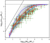 |
Fig. 1. Most massive stellar mass to embedded cluster mass (mmax − Mecl) relation. Red stars denote the observational data listed in Table A.1. Here, 106 synthetic clusters are stochastically sampled from the canonical IMF (the a23m150 IMF model in Table 1), resulting in the density map. The darkness of the region is proportional to the number of the synthetic clusters in that region divided by the total number of synthetic clusters in the same Mecl bin. The average mmax and standard deviation of mmax for each Mecl bin are plotted as the red solid and the blue dashed curves, respectively. The solid line indicates the Mecl = mmax limit and the horizontal dashed line indicates the mup limit of 150 M⊙ (see Sect. 7.4.4). |
The errors and biases of the compiled dataset affect our results as discussed in Sect. 7. In addition, we acknowledge that the stellar mass upper limit is highly uncertain. There are studies suggesting that stars with mass > 300 M⊙ (Crowther et al. 2010; Schneider et al. 2018; Higgins et al. 2022) might be the result of mergers of massive stars (Banerjee et al. 2012a; Oh & Kroupa 2018). However, the mass estimation of massive stars is not the topic of the present study and our conclusion is not affected if we adopt a higher stellar mass estimation. For the present tests, we apply the compiled data along with the measurement errors given by the literature sources. A homogeneous set of observations with higher completeness (the current dataset includes less than about 2% of all the star clusters in the MW; cf. Weidner et al. 2010) and a more reliable mass uncertainty analysis will, in the future, greatly improve the robustness of our study.
3. Test method
3.1. Statistical test
As pointed out in WKP13, the scatter of the observed mmax − Mecl relation appears to be consistent with no intrinsic scatter, which suggests a high degree of self-regulation. To test if nature is indeed significantly more regulated than the stochastic sampling hypothesis, we compare the scatter of the observed relation with that of the synthesised mmax − Mecl relation generated by stochastic sampling.
With forward modelling, a large number of star clusters and their mock observational errors are stochastically generated to form the expected mmax − Mecl density distribution. The mock clusters are set to have a cluster mass distribution similar to the observational dataset, which has a relatively uniform distribution of mass on the logarithmic scale. Therefore, we generate 106 star clusters containing N stars, where N is randomly selected from 20 to 106 with a uniform distribution on the logarithmic scale (we note that the star number and mass distribution are similar; see Sect. 2.2 of WKP13). The observed and synthesised cluster mass distribution are different from the embedded cluster mass distribution in nature with a power index of −2 (Lada & Lada 2003) due to an observational bias towards more massive star clusters.
Given the number of stars in each star cluster, the masses of stars are sampled stochastically (e.g. Kroupa et al. 2013) from a PDF, that is, the assumed IMF. The model results depend on both the sampling method and the IMF. To test the sampling method in such a way that the conclusion does not depend on the assumed shape of the IMF, in the present work we apply two free parameters in the IMF: the high-mass IMF slope, α3, and the stellar mass upper limit, mup. We search for the two parameters that best reproduce the observed mmax − Mecl relation (Sect. 3.2) and compare the scatter of the mock star clusters and the data on the mmax − Mecl plot for the first time. A different IMF prescription, such as a lognormal IMF for low-mass stars (Chabrier 2003), would introduce a systematic change in the mmax − Mecl relation similar to the effect of varying the IMF parameters (α3 and mup) and would not affect our conclusions.
To compare the synthetic star clusters with observations, mock measurement errors of mmax and Mecl are added to the sampled clusters for the first time. The two mass errors are correlated (see discussion in Sect. 7.4) but, as a first step, we assume that they are independent and that they follow one-sided normal distributions with standard deviations being the average observational uncertainties from our complied dataset given in Sect. 2. Doing so results in rare cases with mmax > Mecl in mock observations. Follow-up studies with a uniformly analysed observational dataset allowing accurate forward modelling of the errors are required to resolve this issue.
As the observation and mock observation of synthetic star clusters are now directly comparable, a two-sample test can be performed on the two-dimensional mmax − Mecl relation. To do this, we first measure the variance of mmax values for each Mecl bin for the simulated star clusters. As there is no limit on the number of mock star clusters, the bin size can be arbitrarily small.
An observed star cluster with a known Mecl can then be compared with the mean and the variance of all the mock star clusters in the mass bin that includes the value Mecl. After doing this for all the observed star clusters, we can calculate the likelihood of observing a dataset as extreme as the one we compile from the literature. Finally, since the synthetic mmax − Mecl relation depends on the sampling method, the confidence level with which we can reject the applied sampling hypothesis can be given.
3.2. Initial mass function models
Different IMF assumptions are considered in order to avoid the influence of the IMF model when testing the validity of the sampling methods. The multi-part power-law IMF can be written in general as:
The canonical Kroupa (2001) IMF is a two-part power law with, respectively, mlow, mturn, mturn2 = 0.08, 0.5, 1 [M⊙], α1 = 1.3, α2 = α3 = 2.3, and mup = 150 M⊙. Possible variations of α1 and α2 are discussed in Sect. 7.2. The normalisation parameters, k1, k2, and k3 are adjusted such that the IMF is a continuous function.
The slope of the high-mass IMF, α3, and the physical stellar mass upper limit, mup (=mmax* in Weidner & Kroupa 2006; Weidner et al. 2010), affect the mmax − Mecl relation significantly and both have large uncertainties. Different choices of these parameters are listed in Table 1. We note that α3 = 2.68 is similar to the solar-neighbourhood IMF measured in Scalo (1986) and Kroupa et al. (1993). This is steeper than the IMF in star clusters (cf. Bastian et al. 2010), which is expected for a galaxy-wide IMF made by many star clusters (Kroupa & Weidner 2003). The high-mass IMF slope for the field stars is not accurate due to the large uncertainty on the MW star formation history. A recent study shows that the solar-neighbourhood IMF for massive stars can be consistent with the IMF in star clusters (Mor et al. 2019). For initial stellar populations in star clusters, a flatter slope is favoured and α3 = 2.3 ± 0.7 as is shown by Kroupa (2001, 2002) and Bastian et al. (2010). On the other hand, the estimation of mup depends on the stellar modelling of massive stars and is still under debate (see Sect. 7.4.4). We vary mup to find the best fit with the data without a prior probability distribution.
Best-fit IMF models.
4. Tests of stochastic sampling
4.1. The mock mmax–Mecl relation from stochastic sampling
To discuss the degree of self-regulation in the star formation processes independent of the IMF shape, we not only test with a fiducial IMF model (a23m150 model in Table 1) but also allow freely variable IMF parameters and test parameter values that can best reproduce the observed mmax − Mecl relation (a23m100 and a268m130 models in Table 1 shown in Sects. 4.2.2 and 4.2.3).
Figure 1 shows the distribution of 106 randomly-sampled embedded clusters on the mmax − Mecl relation after applying our fiducial IMF model parameters. The darkness of each region is proportional to the number of clusters in a mmax − Mecl bin divided by the total number of clusters in the same Mecl bin; that is, the darkness denotes the distribution of mmax for a given Mecl. The mean and the standard deviation of mmax for each Mecl bin are also given with the red solid and the blue dashed curves, respectively. Here, the single-sided standard deviations are calculated and shown, assuming that data above and below the mean mmax have different variances, but the upper and lower variances are nearly identical.
The observed star clusters more massive than about 100 M⊙ are systematically below the expected distribution, as is pointed out in Weidner et al. (2010, their Sect. 3.2). A top-light IMF (model a268m130) can result in better agreement, which we discuss in Sect. 4.2. The mass uncertainties of the observations shown in Fig. 1 are large while the distribution of the measurement values is tight, indicating a small intrinsic uncertainty on the star formation process (disfavouring stochastic sampling), an overestimation of the mass uncertainty of observed clusters, and/or a selection bias of the observational dataset.
Figure 2 shows the result after a random observational error is added to each synthetic star cluster. The density distribution shows a larger scatter than the data. The amplitude of this scatter is determined by the sampling method and observational uncertainty. Changing the IMF parameters does not have a significant influence on the scatter but only influences the position and the orientation of the density distribution which is shown in the following section. We note that there are mock clusters with Mecl < mmax (points above the solid line in Fig. 2) simply because we assume for simplicity that the observational uncertainty of Mecl and mmax are independent, which is not accurate, especially for low-mass clusters. However, given the statistical test method described in the following section, the error for the low-mass mock clusters does not significantly affect our conclusions as there are only three clusters in the dataset with Mecl < 10 M⊙.
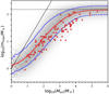 |
Fig. 2. Same as Fig. 1, with the same set of synthetic star clusters (model a23m150), but with mock observational uncertainties added. |
4.2. The p-value
Assuming the null hypothesis that nature behaves in exactly the same way as described by stochastic sampling and that the IMF applied here is correct, here we calculate the likelihood of observing a dataset as extreme as the one we compiled from the literature (i.e. the 100 star clusters listed in Table A.1). We choose a test statistic, n, to be the number of data points in the region above the upper blue dashed curve (hereafter the upper region) or the number of points below the lower blue dashed curve (hereafter the lower region). The expected value of n is 100 × 0.159 = 15.9 points, where 0.159 is the single-sided probability above the standard deviation.
If there are n ≤ 15 points in the upper or lower region, we calculate the likelihood of having ≤n points in that region by applying:
where N = 100 is the total number of data points. The summed terms are the probabilities for each data point and their combination formula while the summation from 0 to n includes all cases as extreme as or more extreme than the observed case (a summation from 0 to N results in 1). On the other hand, if there are n ≥ 16 points in the upper or lower region, we calculate the likelihood of having ≥n points in that region
Then, the joint likelihood or the p-value for a result as equally extreme as or more extreme than the compiled dataset is given by
4.2.1. Model a23m150: the canonical IMF with mup = 150 M⊙
In Fig. 2 there are zero data points in the upper region and 34 in the lower region. The resulting p-value is P = 2 × 10⁻¹³, that is, it is extremely unlikely that the real distribution is given by the synthetic clusters. The corresponding rejection confidence of the stochastic sampling hypothesis is 7σ (calculated in Sect. 4.3).
4.2.2. Model a23m100: the canonical IMF slope with mup = 100 M⊙
As mentioned in Sect. 3, the uncertainty on the assumed IMF shape needs to be taken into account. We first search for the stellar upper mass limit, mup, in Eq. (1), which improves the fit for Mecl > 104 M⊙ as shown in Fig. 3. The best-fit value (with mass changing in steps of 10 M⊙) is mup = 100 M⊙. There are 3 and 25 data points in the upper and lower regions, respectively, and the p-value increases to about 5 × 10⁻⁷. This corresponds to a 4.7σ confidence level to reject the stochastic sampling hypothesis (see Sect. 4.3).
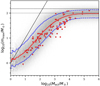 |
Fig. 3. Same as Fig. 2 but for the a23m100 IMF model (Table 1). The additional horizontal dotted line denotes mup = 100 M⊙. |
4.2.3. Model a268m130: non-canonical IMF
We also tested steeper high-mass IMF slopes. Here we allow mup and α3 to vary using a grid with a 10 M⊙ step for different mup and a 0.01 step for different α3. The best-fit combination for the observation is with mup = 130 M⊙ and α3 = 2.68 (model a268m130), in which case the data have six points in both upper and lower regions as shown in Fig. 4. The p-value given by Eq. (4) for this model is still less than 5.7 × 10⁻⁶. As the model fits the data nicely and already achieves the maximum equal number (six) of data points in the upper and lower regions, we can safely conclude that there is no room to further increase the p-value by adjusting IMF parameters for the applied dataset and test statistics. The remaining factor impeding a higher p-value is that the intrinsic variation of the stochastically sampled distribution is too large.
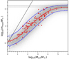 |
Fig. 4. Same as Fig. 2 but for the a268m130 IMF model (Table 1) which best fits the observed mmax − Mecl relation. The additional horizontal dotted line denotes mup = 130 M⊙. |
In addition, the probability of the adjusted α3 should be considered given α3 = 2.3 ± 0.7 for young star clusters (Kroupa 2001). Assuming a normal distribution for the uncertainty of α3, this results in a probability for α3 ≥ 2.68 of about 29%. Therefore, the joint p-value reduces to 5.7 × 10−6 × 29% = 1.7 × 10⁻⁶. The corresponding rejection confidence of the stochastic sampling hypothesis is 4.5σ (see Sect. 4.3).
4.3. Confidence level of rejecting stochastic sampling
Here we estimate the confidence level of rejecting the stochastic sampling hypothesis. According to the Bayesian theory2, two other estimations are needed: the prior probability of the null hypothesis, Pr, and the probability of observing a dataset less extreme than the real observation if the null hypothesis is not true, R. Together with the p-value estimated above, that is, the likelihood of observing a dataset as extreme as the real observation if the null hypothesis is true, P, we can obtain the probability of the null hypothesis being true given the observations, or in other words, the probability of wrongly rejecting the null hypothesis, which is also known as the type I error, A:
with all parameters ranging from 0 to 1.
It is hard to estimate whether nature is more influenced by random processes or feedback self-regulation and the issue is still highly debated. We therefore assign both cases an equal prior probability (i.e. Pr = 0.5). We also assume that half of the observation would be as extreme as the compiled dataset if some other sampling method instead of the stochastic sampling is true (i.e. R = 0.5), because we do not have any information on whether or not the compiled dataset is more extreme than usual. With these values and P ≪ 1, we have
with the p-values given by the a268m130 model in Sect. 4.2 that best reproduces the observed mmax − Mecl relation. The confidence level of rejecting the hypothesis is 1 − A. Given the cumulative normal distribution, this corresponds to a 4.5σ confidence level to reject the stochastic sampling hypothesis. If, on the other hand, the IMF is forced to have the canonical shape with mup ≥ 150 M⊙, then the rejection is at more than 7σ confidence (Sect. 4.2.1, cf. Sect. 7.4.4 for the mass estimation of very massive stars).
5. Optimal sampling
Optimal sampling is a deterministic sampling method that generates stellar masses that populate the IMF with no Poisson noise. The method was introduced by Kroupa et al. (2013) to account for the small scatter of the observations. We refer the readers to Schulz et al. (2015) and Yan et al. (2017) for a further description of optimal sampling and the publicly available GalIMF code3 that optimally populates clusters and galaxies with stars.
Optimal sampling assumes that the formation of stellar populations is perfectly self-regulated and, therefore that a deterministic relationship exists between the mass of a star cluster and the mass of every single star within that cluster. To sample the stellar masses, the IMF is divided into N + 1 sections at mass limits of x1 to xN (where xi > xi + 1). These sections fulfil the mass conservation of the embedded star cluster:
where xlow is the lowest possible stellar mass, 0.08 M⊙. Each section gives exactly one star (therefore, the total number of stars is N):
In other words, if the integrated number of stars between two mass limits equals one, then the cluster must form exactly one star between these two mass limits with the optimally sampled stellar mass given by:
In addition, the value of x1 fulfils
where the theoretical mass limit of the most massive star, xup, is set to 150 M⊙. This set of equations can be solved analytically assuming a two-part power-law IMF (Kroupa 2001) as is done in Yan et al. (2017).
Applying the publicly available GalIMF code, here we sample stars from the canonical IMF4, that is, Eq. (1) with α1 = 1.3 and α2 = α3 = 2.3 (see Sect. 7.2 for IMF variation). The optimally sampled result is shown in Fig. 5, where the mmax − Mecl relation is deterministic.
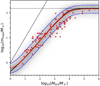 |
Fig. 5. Same as Fig. 2 but with the optimally sampled clusters (the smooth black solid curve) with no intrinsic mmax − Mecl scatter. By assuming a stellar population in an embedded cluster of stellar mass Mecl in an optimal draw from the canonical IMF, the observed distribution is obtained naturally once the observational uncertainties are taken into account. This is not the case for a randomly drawn canonical IMF (Fig. 2). |
We perform the same test as we applied for stochastic sampling in Sect. 4. There are 12 and 24 data points in the upper and lower regions, respectively. The resulting p-value is 0.004, which is three orders of magnitude higher than the result of the stochastic sampling scenario. The total number of observations outside the standard deviation region (12 + 24 = 36) is only 13% larger than the expected number of data in these regions for 100 data points (100 × 31.8% = 32). Adjusting the assumed IMF parameters (as is done for stochastic sampling in Sect. 4.2) would allow us to shift the synthetic mmax − Mecl relation and reach an equal expected number of points in the upper and lower regions and improve the fit. From this, we conclude that optimal sampling is consistent with the observed mmax − Mecl relation and the star formation process appears to have a low level of randomness.
6. Properties of the observed mmax–Mecl relation
6.1. The trend of the data
We visualise the trend of the observational data distribution (Fig. 1) by measuring the mean values of nearby points in both vertical and horizontal directions. The clusters are ranked and grouped by the nearest mmax (or Mecl) values, each group has ten data points, and the neighbouring group differs by only 1 data point. The average values for each group ( or
or  ) are calculated, paired monotonically, and shown in Fig. 6. The error bar of the point is the standard deviation of the mean,
  , where σ10 is the standard deviation of mmax (or Mecl) for a group of 10 data points.
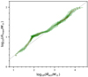 |
Fig. 6. Average position of the observational data for the groups of ten nearest points in the mmax − Mecl relation. The linear grey line highlights that the clusters with a mass of between 101.8 M⊙ = 63 M⊙ and 102.6 M⊙ = 400 M⊙ depart from the linear relation. |
Figure 6 shows a feature above the grey line, that may be related to the stellar and star cluster formation physics. The flatter part of the trend around mmax = 13 M⊙ indicates that the formation of more massive stars may be inhibited at this mass, requiring a more massive star cluster to make the formation possible.
6.2. The scatter of the data
The standard deviation, σ10, of the nearest ten data points for mmax and Mecl (see Sect. 6.1) is plotted for a given mmax in Fig. 7. In addition, the average variances of 104 realisations of mock observations of 100 star clusters generated with the optimal sampling hypothesis (as described in Sect. 5) are shown as solid curves.
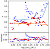 |
Fig. 7. Standard deviation of Mecl (blue triangles) and mmax (red squares) for the groups of ten nearest points in the mmax − Mecl relation. The orange and the blue curves in the upper panel are the synthetic relations assuming optimal sampling of stars. The lower panel shows the difference between the model and the observations. |
The Mecl values of the grouped data points show increased variance at mmax ≈ 13 M⊙ and 100 M⊙. The increase at about 100 M⊙ indicates a possible physical upper limit on stellar mass, mup. The residual of the observation and the optimal sampling model is shown in the lower panel of Fig. 7. The signal-to-noise ratio (S/N5) of the Mecl residual peak at mmax ≈ 13 M⊙ is 13.
The large mmax scatter above 10 M⊙ may be due to the photodissociation radiation produced by these massive stars, such that accretion and growth to larger masses become difficult (Yorke & Sonnhalter 2002; Zinnecker & Yorke 2007). For example, Bonnell et al. (1998) suggest a collisional build-up mechanism for forming massive stars (> 10 M⊙) that requires dense initial conditions that only exist in sufficiently massive star clusters. Thus, these authors predict that the different mechanisms of forming stars may display some structure at ≈10 M⊙. It is also possible that stellar-dynamical encounters eject the most massive stars for embedded clusters with masses in the range between 63 M⊙ and 400 M⊙ (cf. Wang et al. 2019). Indeed, Kroupa et al. (2018) find that the star clusters that are still building up and reach this mass range start forming massive stars but also eject them out of the cluster on a timescale of less than 1 Myr, resulting in a zigzag evolution track towards the upper right in the mmax − Mecl relation, possibly similar to Fig. 6. Both scenarios suggest significant self-regulation in the star formation process.
7. Uncertainty analyses
Although the test in Sect. 4 rejects the stochastic sampling hypothesis with a 4.5σ confidence level (allowing the IMF to deviate from its canonical shape) and at more than 7σ for the canonical IMF shape, any conclusion we can make from these findings depends on the observational uncertainty estimations and data selection bias. This section discusses the effects that may compromise the above rejection.
It is worth noting that any uncertainty or hidden variable that is not accounted for (thus resulting in an underestimated mass measurement uncertainty) increases the scatter of the data points, mimicking stochasticity, which in truth is not present. Only an overestimated uncertainty may compromise the rejection of the stochastic sampling hypothesis.
7.1. Selection bias
It is possible that star clusters with extreme properties, if they do exist, are pre-excluded from the sample; for example, single isolated stars or clusters consisting of only low-mass stars. This potential observational bias would make the resulting mmax − Mecl relation tighter than it really is, which mimics a more regulated star formation process. Even if such clusters are not intentionally excluded, the freak star clusters can be more challenging to observe. A star cluster consisting of only low-mass stars would have a lower luminosity than a normal cluster with the same mass. On the other hand, if a star cluster has an mmax much higher than the value given by the average mmax − Mecl relation, by chance, it is unlikely that the second most massive star in this cluster has a similar mass as its most massive star. This means that, if the most massive star is missed or incorrectly measured in the observation due to, for example, dynamical ejection, stellar evolution, or extinction, the extreme mmax value will also be missed. For normal star clusters on the other hand, even if the most massive star is incorrectly estimated or missed, both sampling methods suggests a few stars with lower but similar masses, reducing the measurement error of mmax.
However, it is likely that freak star clusters do not exist. Stephens et al. (2017) select, in particular, the seven most likely isolated massive stars in the entire Large Magellanic Cloud, each being distant from any known astronomical sources, and followed them up with deeper Hubble Space Telescope observations. In all these seven cases, a large young stellar population is detected in the immediate environment that is distributed in a clustered fashion such that the mmax − Mecl relation is obeyed. In addition, dynamical ejection (Gvaramadze et al. 2011a,b, 2012; Banerjee et al. 2012a,b; Oh & Kroupa 2016), including the two-step ejection process (Pflamm-Altenburg & Kroupa 2010), is known to create apparently isolated massive stars. Therefore, it is likely that all allegedly isolated massive stars are associated with normal star clusters with insufficient observations and should be excluded from our analyses. The stellar associations observed so far with a small number of stars are all in agreement with the non-trivial mmax − Mecl relation (Kirk & Myers 2012).
7.2. Bias from the IMF assumption
For many clusters in our sample, Mecl is estimated by extrapolating the mass of the observed stars assuming a certain IMF. Considering the extreme case where only the mass of the most massive star is measured for star clusters, then the cluster mass would be calculated based only on mmax which results in a deterministic mmax − Mecl relation without any scatter. We try to minimise this effect by excluding clusters with a small number of star detections, but the effect cannot be fully mitigated. For example, the mass of NGC 6611 is estimated based on stars between 6 and 12 M⊙, assuming they account for a certain fraction of the cluster mass derived with a given IMF (Wolff et al. 2007, their Sect. 5). The bias introduced by the IMF assumption depends on the completeness and the mass range of the observed stars, the applied IMF uncertainty, and whether additional Mecl estimations with independent methods (dynamical estimation or from total luminosity) are taken into account. A more homogeneous study would help to better constrain and model this bias.
On the other hand, the shape of the subsolar IMF depends on the metallicity of the stars (Kroupa 2002; Geha et al. 2013; Gennaro et al. 2018; Martín-Navarro et al. 2019; Smith 2020; Yan et al. 2020; Poci et al. 2022; Li et al. 2023). As the observed star clusters do not have the same metallicity, this introduces additional scatter to the expected mmax − Mecl relation, favouring the optimal sampling hypothesis.
7.3. Contamination
Field star contamination is inevitable. Studies employing dynamical and chemical tagging will further reduce the contamination in upcoming surveys.
7.4. Mass uncertainties
7.4.1. Uncertainties from Kirk & Myers
Star clusters with more than 20 detected members (Kirk & Myers 2011, their Table 1) are adopted. The uncertainty on Mecl from Kirk & Myers (2011) is set to be the same as the uncertainty on mmax (which is roughly estimated to be ±50% by Kirk and Myers). Kirk & Myers (2012) find that massive stars can be better described if they assume an older cluster age (2 Myr instead of 1 Myr). This suggests that stars with different masses in the same star cluster may have different average ages and a single age assumption may introduce bias to the mass estimation of these pre-main sequence stars; see also STARFORGE simulations where more massive stars in a star cluster form at a later time (Guszejnov et al. 2022). In addition, the statistical uncertainty on individual stars due to different extinction estimation errors and multiplicity are neglected. An extinction map based on stellar reddening is provided in Kirk & Myers (2011) but the related uncertainty is unknown. A potential multiplicity of the stars could lead to a 20% lower mmax and a 60% higher Mecl than estimated if every star in a cluster is an unresolved equal-mass binary. Furthermore, it is possible that identified star cluster members are either contaminated by field stars or incomplete because of dynamical evolution and that some stars have not formed by the time of observation.
7.4.2. Uncertainties from Stephens et al.
Clusters in Stephens et al. (2017, their Table 6) are included. We adopt the mean cluster mass calculated with cluster ages of 1 and 2.5 Myr. The uncertainties on Mecl consider only the rough age uncertainty on the star cluster when fitting the cluster isochrone. The statistical and/or systematic uncertainties on extinction, distance, the grid of stellar models, and so on are not taken into account. Therefore, this uncertainty can be considered as a lower limit. The adopted mmax uncertainty of about 40% is estimated due to a large number of uncertain effects from the spectral type model, multiplicity, extinction, and stellar age, none of which have been well estimated.
7.4.3. Uncertainties from WKP13
A large number of star clusters are compiled in WKP13 (their Table A.1). We select clusters with younger ages and a large number of detected stars, as described in Sect. 2. According to WKP13, the uncertainty on mmax is estimated assuming a half spectral subclass uncertainty on the most massive star, neglecting potential multiplicity. A physical upper stellar mass limit of 150 M⊙ is implemented in WKP13. More massive stars might be unresolved multiple stars or stars formed through dynamical mergers (Banerjee et al. 2012a; Oh & Kroupa 2018). This upper mass limit would not affect our conclusion, as discussed in the following section.
The uncertainty on Mecl is mostly constituted by the assumption made in WKP13 that all stars could be unresolved binaries and that 50% of the stars may be misidentified as cluster members, suggesting a mass uncertainty of ≈ ± 0.3 dex. This leads to a much higher average uncertainty on Mecl than mmax. In reality, binaries would only lead to a 64% to 68% increase in the estimated system mass for stars between about 0.4 and 55 M⊙ due to the non-linear relation between stellar mass and luminosity, with no increase for extremely massive stars due to the linear relation between stellar mass and luminosity (according to Eq. (12) below); that is, a less than 68% increase in Mecl instead of 100% if all observed stars (mostly massive stars are observed) are unresolved equal-mass binaries. The effect of field star contamination on Mecl may also be lower than previously estimated. Massive stars contribute a large fraction of the cluster mass and are less likely to be missed or contaminated than low-mass stars.
On the other hand, other sources of uncertainty, such as IMF variation, variable extinction, stellar variability, gas expulsion, dynamical evolution, and stellar models, are not fully taken into account and the uncertainties in WKP13 are given as a lower limit. Therefore, it is possible that the adopted uncertainty is realistic.
7.4.4. The masses of very massive stars
The possible mass of the most massive star is still under debate, ranging from 100 to about 300 M⊙. Weidner & Kroupa (2004), Figer (2005), Oey & Clarke (2005), and Koen (2006) suggest an upper limit to the initial masses of stars of about 150 M⊙ (the canonical value), while Crowther et al. (2010, 2016) argue that the limit may be higher given the large systematic uncertainties in the stellar models of the massive stars. Other than the error from extinction and distance measurements, massive stars show strong mass loss and a thick atmosphere, which are difficult to model. Stellar simulations give very different evolution tracks when different amounts of overshooting, rotation, mass loss rate, metallicity, and binary evolution are adopted. The uncertainties are larger for more massive stars (Martins 2015). For example, the evolution tracks of Ekström et al. (2012) failed to reproduce the luminosity and temperature of the stars in the Arches cluster. Yusof et al. (2013) note that, during the advanced phases of their evolution, the very massive stars may have similar luminosities to stars with initial masses of below 120 M⊙, making these stars difficult to distinguish. This leads to the possibility of underestimating the mmax of the Arches cluster. Crowther et al. (2010, 2016) revisited younger star clusters considering the line-blanketed model, and give a higher mass estimation for the stars than WKP13, doubling the mmax value in the case of R136 in 30 Doradus. Applying different stellar evolution models, the mass of R136a1 (i.e. the most massive star in R136) estimated by Brands et al. (2022) greatly exceeds the estimation by Massey & Hunter (1998). On the other hand, the crowded cluster R136 suffers from limited photometric resolution and the very massive stars may turn out to be unresolved multi-stellar systems, as is the case in Pismis 24-1 (Maíz Apellániz et al. 2007). Severe crowding within the core of R136 leads to larger measurement uncertainties and reduces the mass estimations (Rubio-Díez et al. 2017; Kalari et al. 2022). Indeed, stars less massive than about 20 M⊙ are not detected in the central 0.15 pc radius of R136 due to crowding. It is likely that more Wolf-Rayet stars – for example, with 50 M⊙ or 100 M⊙ – exist than those that have been identified and that these stars contribute to the luminosity of unresolved stellar systems. With a linear correlation between mass and luminosity for the most massive stars, unresolved systems can significantly increase the stellar mass measurements. Even if the stars are indeed single stars, the strong stellar wind and highly uncertain mass-loss rate of very massive stars (Higgins et al. 2022) make it impossible to distinguish initial stellar masses above 200 M⊙ on the Hertzsprung–Russell diagram. The wind also reduces the mass of very massive stars to about 150 M⊙ within 1.6 Myr. Therefore, it is likely that a few stars with current masses exceeding the limit of 150 M⊙ but with ages similar to or older than 1.6 Myr (e.g. R136a1 as discussed in Crowther et al. 2010) form through mergers of massive binaries (Banerjee et al. 2012a,b; Oh & Kroupa 2018). Given these considerations, the initial masses of very massive stars are still uncertain.
Nevertheless, a different mass estimation of very massive stars would not significantly affect the present study because the scatter of the mmax − Mecl relation is mainly determined by star clusters with masses below 8000 M⊙ (including 90% of the clusters). The discussion of whether or not the birth masses of the most massive stars can be larger than the canonical 150 M⊙ value is relevant for massive star-burst clusters, such as R136, within which stellar mergers are common, but such clusters are very rare. Therefore, excluding these few data points would affect the best-fit mup value (e.g. Sect. 4.2.3) but not our conclusions.
7.4.5. Correlations between mass estimation errors
The two mass errors are not independent and there are three types of error correlations in general.
– Systematic stellar mass error: The cluster mass is often calculated based on the observed stellar mass, which is extrapolated to the full stellar mass range with an assumed IMF. In this case, stellar model, cluster age, distance, and average dust extinction estimation errors would affect the estimation of both stellar and star-cluster masses with a positive correlation.
– Statistic stellar mass error: random measurement error for mmax contributes to the Mecl error. For example, very massive stars have large uncertainties on their evolution and observational parameters due to strong mass loss and probable binary evolution (Zhang et al. 2005). However, the error correlation is insignificant when the mmax/Mecl ratio is low, which is the case for the majority of the stochastically sampled star clusters. Only about 10% of the star clusters (stochastically sampled from the canonical IMF) have mmax/Mecl > 0.3 and about 4% have mmax/Mecl > 0.5.
– Unresolved multi-stellar system: If a multi-stellar system is unresolved, the mass estimation of the primary star is higher than the correct value while the mass estimation of the star cluster is lower than the correct value, and therefore the errors are anti-correlated.
The values of different types of errors relate differently and non-linearly to the mass estimations of stars and clusters. Ideally, one simulates realistic statistics and systematic uncertainties originating from the stellar model, age estimation, distance, extinction, multiplicity, and so on with detailed forward modelling. However, there are practical difficulties in doing so. Firstly, the uncertainty analyses in the literature are not comprehensive, that is, we do not have detailed information about different types of errors. Usually, only a roughly estimated total error is given, if at all. Secondly, the measurements are adopted from different studies applying different methods of mass estimation with different uncertainties, such that there is no uniform way to simulate mock uncertainties that can represent the dataset. Thirdly, the observational uncertainty on freak star clusters (Sect. 7.1) cannot be estimated because these latter are not observed and only exist in the mock dataset.
7.4.6. Non-Gaussian mass error distribution
We test the additional scenario whereby mock mass measurement errors follow a truncated normal distribution clipped to the range 0 to 2σ. Again, the upper and lower variances are different (see Sect. 2), and therefore the upper and lower clip values are calculated separately. The change reduces the scatter of the synthetic mmax − Mecl relation and increases the p-value of our two-sample test. An equal number of data points in the upper and lower regions can increase to seven at most, with slightly adjusted IMF parameters. The resulting confidence level for rejecting the stochastic sampling hypothesis is reduced to 4σ for the case allowing mup and α3 to deviate from the canonical IMF, which is still significant.
7.5. Conditions for stochastic sampling to reproduce the observed mmax–Mecl relation
Considering that the Mecl uncertainties are not well-estimated in much of the adopted literature, we explore what would be the correct mean Mecl uncertainty if the stochastic sampling hypothesis were correct. We find that for the stochastically generated star clusters to reproduce the observed tight mmax − Mecl relation, there needs to be a high probability (> 50%) of omitting the most massive stars in our mock observation and that the applied cluster mass uncertainties must be much smaller than the average value of the observational dataset. Specifically, if the average uncertainty on Mecl is the same as the average uncertainty on mmax on the logarithmic scale (i.e. about 0.15 dex instead of 0.3 dex), the resulting mock observations would have a similar scatter to the observed points.
However, Sects. 7.4.1–7.4.3 demonstrate that the adopted mass uncertainties are often given as a lower limit. Therefore, these requirements are not likely to be fulfilled.
8. Discussion
8.1. Previous studies
Reproducing the mean trend of the mmax − Mecl relation (Cerviño et al. 2013; Hirai et al. 2021) is possible with both sampling hypotheses but the small scatter on the mmax − Mecl relation favours optimal sampling. A possibly larger measurement uncertainty of the adopted dataset, as is suggested by Krumholz (2014) and Sects. 7.4.1–7.4.3 above, would suggest an even smaller intrinsic scatter of the mmax − Mecl relation and strengthen the argument favouring optimal sampling.
We note that a test between deterministic sampling and stochastic sampling (e.g. the present work) is different from a test between stochastic sampling and stochastic sampling with a cluster-mass-dependent truncation for the mass of the most massive star (e.g. Hermanowicz et al. 2013). Earlier works studying the mmax − Mecl relation assume the truncated stochastic sampling scenario (e.g. Weidner & Kroupa 2006, their sorted random sampling), which is claimed to be ruled out by many studies (e.g. Corbelli et al. 2009; Fumagalli et al. 2011; Andrews et al. 2013, 2014; Dib et al. 2017). However, these latter are not falsifications of optimal sampling, which is a pure deterministic sampling (Eqs. (8) and (9), see also Kroupa et al. 2013, their Eq. (4.9), Schulz et al. 2015, their Eqs. (6) and (7)) and is distinct from stochastic sampling under a deterministic truncation. For example, Weidner et al. (2010) discuss the observational mmax − Mecl relation, and therefore their mmax corresponds to ‘the mass’ of the most-massive star and the best-fit relation is consistent with the observation by definition. However, if the observational mmax is taken as ‘the mass limit’ of the most-massive star for stochastic sampling, the stochastically sampled most massive star would be systematically less massive than mmax, and therefore inconsistent with the observations. Similarly, according to the optimal sampling hypothesis, star clusters of 100, 400, and 1000 M⊙, and with (one-tenth of) the solar metallicity must have a most-massive star of approximately 8 (9), 20 (22), and 36 (40) M⊙, respectively (calculated by the open-source GalIMF code, Yan et al. 2017), which are in good agreement with the observations presented by Koda et al. (2012).
In summary, truncated statistical sampling is not directly related to the discussion of whether the star formation process is highly self-regulated. A significantly tight mmax − Mecl relation can and can only exist because of optimal sampling instead of truncated random sampling, which is in agreement with previous studies.
8.2. Practical considerations
The deterministic optimal sampling method is useful when one aims to study the evolution of an ‘average’ stellar population closely resembling the IMF. The optimally sampled stellar population is not only a fair sample of the IMF but also has a mass error smaller than the mass of the lowest-mass star, 0.08 M⊙. In comparison, the stochastic sampling hypothesis contradicts mass conservation. Given the total mass of a molecular cloud and a star formation efficiency (which may be universal), what is being constrained is the mass instead of the number of the stars that can form in that cloud. Macroscopic physics, as we know it, is not stochastic. There are a variety of treatments regarding when to stop the random drawing of stars in order to approximate mass conservation to some level, but mass conservation and reproduction of the IMF cannot be simultaneously fulfilled with stochastic sampling (Smith 2021, their Sect. 2). Therefore, various mass-transfer schemes (transfer of mass up to the mass of the assumed stellar-mass upper limit) between nearby gas or star particles are applied to enforce the mass conservation in simulations applying random sampling (e.g. references listed in Sect. 1).
Optimal sampling is also much more efficient in situations when only the masses of the most massive stars are of interest (Applebaum et al. 2020; Hislop et al. 2022) because the numbers are deterministic and can be given analytically (Eqs. (7)–(10)). However, in the case of stochastic sampling, sampling only the massive stars, such as in Gatto et al. (2017), does not follow the probabilistic interpretation of the IMF where the formation of stars is an independent process. Therefore, one should always finish sampling all the stars in a star cluster before the most massive stars can be identified without bias (e.g. the method described in Geen et al. 2018, their Sect. 2.4). This leads to a significant cost difference between the two sampling methods.
On the other hand, the optimal sampling hypothesis faces a fundamental problem: the total mass of a real single formation event of a star cluster cannot be well defined because stars do not form in one instance and there may be multiple populations of stars formed (or captured) in the same star cluster (Pflamm-Altenburg & Kroupa 2007, 2008, 2009; Kroupa et al. 2018; Wang et al. 2020; Wirth et al. 2022). In addition, optimal sampling cannot be directly applied to star particles that represent multiple star clusters or a fraction of a star cluster. This problem can be bypassed by stochastic sampling from a list of optimally sampled stellar masses of a galaxy (i.e. OSGIMF, Yan et al. 2017) and may eventually be resolved by galaxy simulation models where the stellar particle represents the true cluster mass.
8.3. Properties of the star forming clouds
Assuming a star formation efficiency of 33%, the total mass of the pre-cluster molecular cloud, Mcl, can be estimated. The scaling relation between Mecl and the pre-cluster molecular cloud core density, ρcl, from Yan et al. (2017, their Eq. (7)) is applied to estimate ρcl, that is
![$$ \begin{aligned} \log _{10}(\rho _{\mathrm{cl} }\ [M_\odot /\mathrm{pc}^3]) = 0.61\cdot \log _{10}(M_{\rm ecl}\ [M_\odot ]) + 2.85. \end{aligned} $$](/articles/aa/full_html/2023/02/aa44919-22/aa44919-22-eq14.gif)
Therefore, the mmax − Mecl relation results in the relations of these quantities, as is shown in Fig. 8.
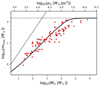 |
Fig. 8. Same as Fig. 5 but for the pre-cluster molecular cloud mass, Mcl, and cloud core density, ρcl, assuming a star formation efficiency of 33% and Eq. (11). The thick curve is given by the optimal sampling hypothesis (Sect. 5). |
In addition, the bolometric luminosity, Lbol, of the most massive star is derived following the mass–luminosity relation summarised in Yan et al. (2019, their Eq. (1)), following Duric (2004, their Chap. 1.3.8) for the low-mass stars and Salaris & Cassisi (2006, their Chap. 5.7) for the stars more massive than about 2 M⊙
where m is the stellar initial mass. Salaris & Cassisi (2006) argue that, for more massive stars (> 20 M⊙), L ∝ M because radiation pressure is dominating the total pressure instead of gas pressure. However, the exact mass boundary within which we can apply a linear L − M relation is not provided. Observations for stars up to 50 M⊙ suggest a L − M relation with a power-law index of about 2.8 instead of 1 (Vitrichenko et al. 2007 and up to 64 M⊙ according to Eker et al. 2018, their Table 7). For simplicity, here we assume the widely applied power-law index of 3.5 for stars below 55.41 M⊙ and a linear L − M relation for more massive stars following Yan et al. (2019). The derived Lbol values and the ratios between Mcl and Lbol are shown in Fig. 9.
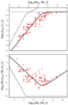 |
Fig. 9. Same as Figs. 5 and 8 but for the bolometric luminosity (upper panel) and the mass-to-light ratio (lower panel). The horizontal coordinates of the upper and lower panel are identical to Figs. 5 and 8 (Mcl = 3 Mecl). |
Finally, the total combined bolometric luminosity of all the optimally sampled stars in a young star cluster is calculated, assuming that the pre-main sequence stars have a bolometric luminosity equal to the zero age main sequence (ZAMS) stars given by Eq. (12). The relation predicted by the optimal sampling hypothesis is compared with the observed mass, Mfwhm, and bolometric luminosity within the FWHM source sizes of the star-forming dense molecular clumps (Urquhart et al. 2022, their HII region related clumps) in Fig. 10, assuming Mcl = Mfwhm.
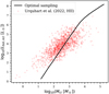 |
Fig. 10. Total stellar bolometric luminosity–pre-cluster molecular cloud mass relation. The solid curve shows the prediction from the optimal sampling method, where the cluster mass relates to the mass of each star formed in that cluster deterministically, according to Eqs. (7)–(10). The total stellar luminosity is calculated with Eq. (12). The red circles are the observational data adopted from Urquhart et al. (2022); specifically their clumps related to HII regions. |
The optimal sampling model is in qualitative agreement with the data (Fig. 10), which include complex radiation processes and a contribution from accretion luminosity. The model, in contrast, counts only the ZAMS luminosities of all stars in the embedded cluster, assuming them to appear instantly at the same time, while star-formation might proceed over 1 Myr (Sect. 7.4.1). In addition, massive stars can already be ejected from the cloud within 1 Myr (Kroupa et al. 2018). These effects result in a lower observed luminosity than our model for massive clusters. On the other hand, the observational data systematically become more luminous than the optimal sampling model towards smaller cloud mass Mcl. This is likely a consequence of the following physics: at the massive end, most of the bolometric luminosity comes from the massive stars, which are already on the main sequence when they become detectable in HII regions. The model therefore well represents these data. Low-mass embedded clusters, on the other had, are predominantly populated by low-mass stars. These are, when they become visible, still contracting onto the main sequence with significantly larger luminosities when very young. It will be an interesting problem to include pre-main sequence evolutionary tracks into the optimal sampling model to test, in the future, whether the observational data shown in Fig. 10 better agree with such a model. At the low-mass cluster end, the optimal sampling model does not expect the formation of massive stars in these clusters, while some observed low-mass clumps appear to have HII region features. The ionising radiation responsible for creating the HII region may be due to low-mass pre-main sequence stars producing a higher ionising flux than their ZAMS counterparts due to their flaring activity (e.g. Raetz et al. 2020).
9. Conclusions
In this study, we demonstrate that the stochastic sampling hypothesis fails to reproduce the small scatter of the observed mmax − Mecl relation such that the hypothesis is rejected at a 4.5σ significance level if: the measurement uncertainties of mmax and Mecl are not overestimated; the compiled dataset is unbiased; and if the IMF can be adjusted. If, on the other hand, the IMF is fixed to the canonical form and mup ≥ 150 M⊙, then the data are inconsistent with random sampling with > 7σ confidence. If the adopted mass uncertainties are underestimated, which is the case when certain uncertainties are omitted, the conclusion becomes stronger. In comparison, optimal sampling from an invariant canonical IMF and without an intrinsic dispersion of mmax values for a given Mecl describes the observed mmax − Mecl relation naturally.
The optimal sampling model predicts a strong correlation between the bolometric luminosity of a young stellar population and the mass of the embedded cluster. We calculate this relation assuming a freshly hatched optimally sampled stellar population on the ZAMS. The correlation agrees qualitatively well (Fig. 10) with the data from the ATLASGAL survey (Urquhart et al. 2022). Future modelling will likely improve the agreement once pre-main sequence stellar evolution tracks are incorporated into the evolution of the bolometric luminosity of low-mass stars.
In addition, we discover a large number of clusters with mmax ≈ 13 M⊙. This may indicate that the formation of more massive stars is inhibited beyond 13 M⊙ and/or that there is a strong dynamical ejection for the most massive stars for embedded clusters with stellar masses in the range of about 63 to 400 M⊙, supporting significant self-regulation in the star formation process.
A homogeneous and consistent observational survey of embedded clusters and their stellar content would help to improve the reliability of our statistical test by providing a more reliable uncertainty analysis. Studies examining the properties of dwarf galaxies (as mentioned in Sect. 1) will continue to provide us with constraints on the self-regulation in the star formation process. For example, if stars were stochastically sampled, then the integrated galaxy-wide IMF of many dwarf galaxies would be the same as the canonical IMF (cf. Lee et al. 2009), meaning that they would have the same supernova formation efficiency as massive galaxies (cf. Zhang et al. 2021) and that their chemical evolution would be understandable with an invariant canonical IMF (cf. Yan et al. 2020; Mucciarelli et al. 2021). See also Kroupa & Jerabkova (2021, their Sect. 1.6.3) for a further discussion of these tests.
In conclusion, we still do not have a comprehensive theory of how stars form. Nature is deterministic, and so star formation cannot be stochastic. However, as we do not know all the variables (e.g. rotation, temperature) of the embedded-cluster-forming molecular cloud clump, this lack of knowledge would transpire as an apparent stochasticity on top of the optimal sampling process, such that the practical sampling method could be in between the statistical and optimal sampling extremes. The Python GalIMF code, which performs optimal sampling for star clusters and entire galaxies, is publicly available (see Sect. 5).
An embedded cluster refers to a correlated star formation event, i.e. a gravitationally driven collective process of transformation of the interstellar gaseous matter into stars in molecular-cloud overdensities on a spatial scale of about one pc and within about 1 Myr (Lada & Lada 2003; Kroupa et al. 2013; Megeath et al. 2016). The value Mecl is the mass of all stars formed in the embedded cluster.

See ‘example_star_cluster_IMF.py’ in the GalIMF package. The code is also capable of optimally sampling stars from all the star clusters in a galaxy formed within a correlated 10 Myr star formation epoch (Yan et al. 2017) by implementing an empirical embedded cluster mass distribution, as is demonstrated by ‘example_galaxy_wide_IMF.py’ in the GalIMF package.
![$ S/N = \left(\frac{\mathrm{MAX}[\mathrm{ABS[residual]}]}{\mathrm{AVE}\left[\mathrm{ABS[residual]}\right]}\right)^2 $](/articles/aa/full_html/2023/02/aa44919-22/aa44919-22-eq17.gif)
Acknowledgments
Z.Y. acknowledges support from National Natural Science Foundation of China under grant number 12203021, the Jiangsu Funding Program for Excellent Postdoctoral Talent under grant number 2022ZB54, the Fundamental Research Funds for the Central Universities under grant number 0201/14380049, the National Natural Science Foundation of China under grants No. 12041305 and 12173016, the Program for Innovative Talents, Entrepreneurs in Jiangsu, the science research grants from the China Manned Space Project with NO.CMS-CSST-2021-A08 (IMF).
References
- Adams, F. C., & Fatuzzo, M. 1996, ApJ, 464, 256 [NASA ADS] [CrossRef] [Google Scholar]
- Anders, P., & Fritze-v Alvensleben, U. 2003, A&A, 401, 1063 [NASA ADS] [CrossRef] [EDP Sciences] [Google Scholar]
- André, P., Revéret, V., Könyves, V., et al. 2016, A&A, 592, A54 [NASA ADS] [CrossRef] [EDP Sciences] [Google Scholar]
- Andrews, J. E., Calzetti, D., Chandar, R., et al. 2013, ApJ, 767, 51 [NASA ADS] [CrossRef] [Google Scholar]
- Andrews, J. E., Calzetti, D., Chandar, R., et al. 2014, ApJ, 793, 4 [NASA ADS] [CrossRef] [Google Scholar]
- Applebaum, E., Brooks, A. M., Quinn, T. R., & Christensen, C. R. 2020, MNRAS, 492, 8 [CrossRef] [Google Scholar]
- Banerjee, S., Kroupa, P., & Oh, S. 2012a, MNRAS, 426, 1416 [NASA ADS] [CrossRef] [Google Scholar]
- Banerjee, S., Kroupa, P., & Oh, S. 2012b, ApJ, 746, 15 [Google Scholar]
- Bastian, N., Covey, K. R., & Meyer, M. R. 2010, ARA&A, 48, 339 [Google Scholar]
- Bonnell, I. A., Bate, M. R., Clarke, C. J., & Pringle, J. E. 1997, MNRAS, 285, 201 [NASA ADS] [CrossRef] [Google Scholar]
- Bonnell, I. A., Bate, M. R., & Zinnecker, H. 1998, MNRAS, 298, 93 [Google Scholar]
- Bonnell, I. A., Clarke, C. J., Bate, M. R., & Pringle, J. E. 2001, MNRAS, 324, 573 [NASA ADS] [CrossRef] [Google Scholar]
- Bonnell, I. A., Bate, M. R., & Vine, S. G. 2003, MNRAS, 343, 413 [NASA ADS] [CrossRef] [Google Scholar]
- Bonnell, I. A., Vine, S. G., & Bate, M. R. 2004, MNRAS, 349, 735 [Google Scholar]
- Borrow, J., Schaller, M., Bahe, Y. M., et al. 2022, MNRAS, submitted [arXiv:2211.08442] [Google Scholar]
- Brands, S. A., de Koter, A., Bestenlehner, J. M., et al. 2022, A&A, 663, A36 [Google Scholar]
- Carigi, L., & Hernandez, X. 2008, MNRAS, 390, 582 [NASA ADS] [CrossRef] [Google Scholar]
- Cerviño, M., & Luridiana, V. 2004, A&A, 413, 145 [NASA ADS] [CrossRef] [EDP Sciences] [Google Scholar]
- Cerviño, M., Román-Zúñiga, C., Luridiana, V., et al. 2013, A&A, 553, A31 [NASA ADS] [CrossRef] [EDP Sciences] [Google Scholar]
- Chabrier, G. 2003, PASP, 115, 763 [Google Scholar]
- Corbelli, E., Verley, S., Elmegreen, B. G., & Giovanardi, C. 2009, A&A, 495, 479 [NASA ADS] [CrossRef] [EDP Sciences] [Google Scholar]
- Crowther, P. A., Schnurr, O., Hirschi, R., et al. 2010, MNRAS, 408, 731 [Google Scholar]
- Crowther, P. A., Caballero-Nieves, S. M., Bostroem, K. A., et al. 2016, MNRAS, 458, 624 [Google Scholar]
- Crutcher, R. M., & Troland, T. H. 2007, IAU Symp., 237, 141 [NASA ADS] [Google Scholar]
- da Silva, R. L., Fumagalli, M., & Krumholz, M. 2012, ApJ, 745, 145 [CrossRef] [Google Scholar]
- Dib, S., Schmeja, S., & Hony, S. 2017, MNRAS, 464, 1738 [NASA ADS] [CrossRef] [Google Scholar]
- Dinnbier, F., Kroupa, P., & Anderson, R. I. 2022, A&A, 660, A61 [NASA ADS] [CrossRef] [EDP Sciences] [Google Scholar]
- Duric, N. 2004, Advanced Astrophysics (Cambridge: Cambridge University Press) [Google Scholar]
- Eker, Z., Bakış, V., Bilir, S., et al. 2018, MNRAS, 479, 5491 [NASA ADS] [CrossRef] [Google Scholar]
- Ekström, S., Georgy, C., Eggenberger, P., et al. 2012, A&A, 537, A146 [Google Scholar]
- Elmegreen, B. G. 2000, ApJ, 539, 342 [NASA ADS] [CrossRef] [Google Scholar]
- Elmegreen, B. G. 2006, ApJ, 648, 572 [Google Scholar]
- Emerick, A., Bryan, G. L., & Mac Low, M.-M. 2019, MNRAS, 482, 1304 [NASA ADS] [CrossRef] [Google Scholar]
- Figer, D. F. 2005, Nature, 434, 192 [Google Scholar]
- Fumagalli, M., da Silva, R. L., & Krumholz, M. R. 2011, ApJ, 741, L26 [NASA ADS] [CrossRef] [Google Scholar]
- Gatto, A., Walch, S., Naab, T., et al. 2017, MNRAS, 466, 1903 [NASA ADS] [CrossRef] [Google Scholar]
- Geen, S., Watson, S. K., Rosdahl, J., et al. 2018, MNRAS, 481, 2548 [CrossRef] [Google Scholar]
- Geha, M., Brown, T. M., Tumlinson, J., et al. 2013, ApJ, 771, 29 [NASA ADS] [CrossRef] [Google Scholar]
- Gennaro, M., Tchernyshyov, K., Brown, T. M., et al. 2018, ApJ, 855, 20 [NASA ADS] [CrossRef] [Google Scholar]
- González-Lópezlira, R. A., Pflamm-Altenburg, J., & Kroupa, P. 2012, ApJ, 761, 124 [CrossRef] [Google Scholar]
- Guszejnov, D., Grudić, M. Y., Offner, S. S. R., et al. 2022, MNRAS, 515, 4929 [NASA ADS] [CrossRef] [Google Scholar]
- Gutcke, T. A., Pakmor, R., Naab, T., & Springel, V. 2021, MNRAS, 501, 5597 [NASA ADS] [Google Scholar]
- Gvaramadze, V. V., Kniazev, A. Y., Kroupa, P., & Oh, S. 2011a, A&A, 535, A29 [NASA ADS] [CrossRef] [EDP Sciences] [Google Scholar]
- Gvaramadze, V. V., Pflamm-Altenburg, J., & Kroupa, P. 2011b, A&A, 525, A17 [NASA ADS] [CrossRef] [EDP Sciences] [Google Scholar]
- Gvaramadze, V. V., Weidner, C., Kroupa, P., & Pflamm-Altenburg, J. 2012, MNRAS, 424, 3037 [NASA ADS] [CrossRef] [Google Scholar]
- Hacar, A., Tafalla, M., & Alves, J. 2017, A&A, 606, A123 [NASA ADS] [CrossRef] [EDP Sciences] [Google Scholar]
- Hermanowicz, M. T., Kennicutt, R. C., & Eldridge, J. J. 2013, MNRAS, 432, 3097 [NASA ADS] [CrossRef] [Google Scholar]
- Higgins, E. R., Vink, J. S., Sabhahit, G. N., & Sander, A. A. C. 2022, MNRAS, 516, 4052 [NASA ADS] [CrossRef] [Google Scholar]
- Hirai, Y., Fujii, M. S., & Saitoh, T. R. 2021, PASJ, 73, 1036 [NASA ADS] [CrossRef] [Google Scholar]
- Hislop, J. M., Naab, T., Steinwandel, U. P., et al. 2022, MNRAS, 509, 5938 [Google Scholar]
- Hsu, W.-H., Hartmann, L., Allen, L., et al. 2012, ApJ, 752, 59 [Google Scholar]
- Hsu, W.-H., Hartmann, L., Allen, L., et al. 2013, ApJ, 764, 114 [Google Scholar]
- Hu, C.-Y. 2019, MNRAS, 483, 3363 [NASA ADS] [CrossRef] [Google Scholar]
- Hu, C.-Y., Naab, T., Glover, S. C. O., Walch, S., & Clark, P. C. 2017, MNRAS, 471, 2151 [NASA ADS] [CrossRef] [Google Scholar]
- Kalari, V. M., Horch, E. P., Salinas, R., et al. 2022, ApJ, 935, 162 [NASA ADS] [CrossRef] [Google Scholar]
- Kirk, H., & Myers, P. C. 2011, ApJ, 727, 64 [Google Scholar]
- Kirk, H., & Myers, P. C. 2012, ApJ, 745, 131 [NASA ADS] [CrossRef] [Google Scholar]
- Koda, J., Yagi, M., Boissier, S., et al. 2012, ApJ, 749, 20 [NASA ADS] [CrossRef] [Google Scholar]
- Koen, C. 2006, MNRAS, 365, 590 [NASA ADS] [CrossRef] [Google Scholar]
- Köppen, J., Weidner, C., & Kroupa, P. 2007, MNRAS, 375, 673 [CrossRef] [Google Scholar]
- Kroupa, P. 2001, MNRAS, 322, 231 [NASA ADS] [CrossRef] [Google Scholar]
- Kroupa, P. 2002, Science, 295, 82 [Google Scholar]
- Kroupa, P. 2015, Can. J. Phys., 93, 169 [NASA ADS] [CrossRef] [Google Scholar]
- Kroupa, P., & Bouvier, J. 2003, MNRAS, 346, 343 [NASA ADS] [CrossRef] [Google Scholar]
- Kroupa, P., & Jerabkova, T. 2021, Star-formation Rates of Galaxies. Chapter 2: The Initial Mass Function of Stars and the Star-formation Rates of Galaxies, eds. V. Buat, & A. Zezas (Cambridge: Cambridge University Press) [Google Scholar]
- Kroupa, P., & Weidner, C. 2003, ApJ, 598, 1076 [NASA ADS] [CrossRef] [Google Scholar]
- Kroupa, P., Tout, C. A., & Gilmore, G. 1993, MNRAS, 262, 545 [NASA ADS] [CrossRef] [Google Scholar]
- Kroupa, P., Aarseth, S., & Hurley, J. 2001, MNRAS, 321, 699 [NASA ADS] [CrossRef] [Google Scholar]
- Kroupa, P., Weidner, C., Pflamm-Altenburg, J., et al. 2013, in Planets, Stars and Stellar Systems. Volume 5: Galactic Structure and Stellar Populations, eds. T. D. Oswalt, & G. Gilmore (Dordrecht: Springer Science+Business Media), 115 [Google Scholar]
- Kroupa, P., Jeřábková, T., Dinnbier, F., Beccari, G., & Yan, Z. 2018, A&A, 612, A74 [NASA ADS] [CrossRef] [EDP Sciences] [Google Scholar]
- Krumholz, M. R. 2014, Phys. Rep., 539, 49 [Google Scholar]
- Lada, C. J., & Lada, E. A. 2003, ARA&A, 41, 57 [Google Scholar]
- Lahén, N., Naab, T., Johansson, P. H., et al. 2020, ApJ, 891, 2 [CrossRef] [Google Scholar]
- Lahén, N., Naab, T., Kauffmann, G., et al. 2022, MNRAS, submitted [arXiv:2211.15705] [Google Scholar]
- Larson, R. B. 1982, MNRAS, 200, 159 [NASA ADS] [Google Scholar]
- Larson, R. B. 2003, ASP Conf. Ser., 287, 65 [NASA ADS] [Google Scholar]
- Lee, J. C., Gil de Paz, A., Tremonti, C., et al. 2009, ApJ, 706, 599 [NASA ADS] [CrossRef] [Google Scholar]
- Li, Z.-Y., & Nakamura, F. 2006, ApJ, 640, L187 [NASA ADS] [CrossRef] [Google Scholar]
- Li, J., Liu, C., Zhang, Z. Y., et al. 2023, Nature, 613, 460 [NASA ADS] [CrossRef] [Google Scholar]
- Maíz Apellániz, J., Walborn, N. R., Morrell, N. I., Niemela, V. S., & Nelan, E. P. 2007, ApJ, 660, 1480 [Google Scholar]
- Marks, M., & Kroupa, P. 2012, A&A, 543, A8 [NASA ADS] [CrossRef] [EDP Sciences] [Google Scholar]
- Marks, M., Kroupa, P., Dabringhausen, J., & Pawlowski, M. S. 2012, MNRAS, 422, 2246 [NASA ADS] [CrossRef] [Google Scholar]
- Martín-Navarro, I., Lyubenova, M., van de Ven, G., et al. 2019, A&A, 626, A124 [Google Scholar]
- Martins, F. 2015, Astrophys. Space Sci. Lib., 412, 9 [NASA ADS] [CrossRef] [Google Scholar]
- Massey, P., & Hunter, D. A. 1998, ApJ, 493, 180 [NASA ADS] [CrossRef] [Google Scholar]
- Megeath, S. T., Gutermuth, R., Muzerolle, J., et al. 2016, AJ, 151, 5 [Google Scholar]
- Minelli, A., Mucciarelli, A., Romano, D., et al. 2021, ApJ, 910, 114 [CrossRef] [Google Scholar]
- Moe, M., & Di Stefano, R. 2017, ApJS, 230, 15 [Google Scholar]
- Mor, R., Robin, A. C., Figueras, F., Roca-Fàbrega, S., & Luri, X. 2019, A&A, 624, L1 [NASA ADS] [CrossRef] [EDP Sciences] [Google Scholar]
- Mucciarelli, A., Massari, D., Minelli, A., et al. 2021, Nat. Astron., 5, 1247 [NASA ADS] [CrossRef] [Google Scholar]
- Oey, M. S., & Clarke, C. J. 2005, ApJ, 620, L43 [NASA ADS] [CrossRef] [Google Scholar]
- Oh, S., & Kroupa, P. 2012, MNRAS, 424, 65 [NASA ADS] [CrossRef] [Google Scholar]
- Oh, S., & Kroupa, P. 2016, A&A, 590, A107 [NASA ADS] [CrossRef] [EDP Sciences] [Google Scholar]
- Oh, S., & Kroupa, P. 2018, MNRAS, 481, 153 [NASA ADS] [CrossRef] [Google Scholar]
- Oh, S., Kroupa, P., & Pflamm-Altenburg, J. 2015, ApJ, 805, 92 [Google Scholar]
- Pflamm-Altenburg, J., & Kroupa, P. 2007, MNRAS, 375, 855 [NASA ADS] [CrossRef] [Google Scholar]
- Pflamm-Altenburg, J., & Kroupa, P. 2008, IAU Symp., 246, 71 [NASA ADS] [Google Scholar]
- Pflamm-Altenburg, J., & Kroupa, P. 2009, MNRAS, 397, 488 [CrossRef] [Google Scholar]
- Pflamm-Altenburg, J., & Kroupa, P. 2010, MNRAS, 404, 1564 [NASA ADS] [Google Scholar]
- Pflamm-Altenburg, J., Weidner, C., & Kroupa, P. 2007, ApJ, 671, 1550 [NASA ADS] [CrossRef] [Google Scholar]
- Pflamm-Altenburg, J., Weidner, C., & Kroupa, P. 2009, MNRAS, 395, 394 [CrossRef] [Google Scholar]
- Pflamm-Altenburg, J., González-Lópezlira, R. A., & Kroupa, P. 2013, MNRAS, 435, 2604 [CrossRef] [Google Scholar]
- Piskunov, A. E., Kharchenko, N. V., Schilbach, E., et al. 2009, A&A, 507, L5 [NASA ADS] [CrossRef] [EDP Sciences] [Google Scholar]
- Poci, A., McDermid, R. M., Lyubenova, M., et al. 2022, MNRAS, 514, 3660 [NASA ADS] [CrossRef] [Google Scholar]
- Raetz, S., Stelzer, B., & Scholz, A. 2020, Astron. Nachr., 341, 519 [NASA ADS] [CrossRef] [Google Scholar]
- Recchi, S., Calura, F., & Kroupa, P. 2009, A&A, 499, 711 [NASA ADS] [CrossRef] [EDP Sciences] [Google Scholar]
- Revaz, Y., Arnaudon, A., Nichols, M., Bonvin, V., & Jablonka, P. 2016, A&A, 588, A21 [NASA ADS] [CrossRef] [EDP Sciences] [Google Scholar]
- Rubio-Díez, M. M., Najarro, F., García, M., & Sundqvist, J. O. 2017, IAU Symp., 329, 131 [Google Scholar]
- Salaris, M., & Cassisi, S. 2006, Evolution of Stars and Stellar Populations (Wiley-VCH) [Google Scholar]
- Scalo, J. M. 1986, Fund. Cosm. Phys, 11, 1 [NASA ADS] [Google Scholar]
- Schneider, F. R. N., Sana, H., Evans, C. J., et al. 2018, Science, 359, 69 [NASA ADS] [CrossRef] [Google Scholar]
- Schulz, C., Pflamm-Altenburg, J., & Kroupa, P. 2015, A&A, 582, A93 [NASA ADS] [CrossRef] [EDP Sciences] [Google Scholar]
- Shu, F. H., Adams, F. C., & Lizano, S. 1987, ARA&A, 25, 23 [Google Scholar]
- Silk, J. 1995, ApJ, 438, L41 [NASA ADS] [CrossRef] [Google Scholar]
- Smith, R. J. 2020, ARA&A, 58, 577 [NASA ADS] [CrossRef] [Google Scholar]
- Smith, M. C. 2021, MNRAS, 502, 5417 [NASA ADS] [CrossRef] [Google Scholar]
- Smith, M. C., Bryan, G. L., Somerville, R. S., et al. 2021, MNRAS, 506, 3882 [NASA ADS] [CrossRef] [Google Scholar]
- Sormani, M. C., Treß, R. G., Klessen, R. S., & Glover, S. C. O. 2017, MNRAS, 466, 407 [NASA ADS] [CrossRef] [Google Scholar]
- Stephens, I. W., Gouliermis, D., Looney, L. W., et al. 2017, ApJ, 834, 94 [Google Scholar]
- Su, K.-Y., Hopkins, P. F., Hayward, C. C., et al. 2018, MNRAS, 480, 1666 [NASA ADS] [Google Scholar]
- Urquhart, J. S., Wells, M. R. A., Pillai, T., et al. 2022, MNRAS, 510, 3389 [NASA ADS] [CrossRef] [Google Scholar]
- Vázquez, G. A., & Leitherer, C. 2005, ApJ, 621, 695 [Google Scholar]
- Vitrichenko, E. A., Nadyozhin, D. K., & Razinkova, T. L. 2007, Astron. Lett., 33, 251 [NASA ADS] [CrossRef] [Google Scholar]
- Wang, L., & Jerabkova, T. 2021, A&A, 655, A71 [NASA ADS] [CrossRef] [EDP Sciences] [Google Scholar]
- Wang, L., Kroupa, P., & Jerabkova, T. 2019, MNRAS, 484, 1843 [NASA ADS] [CrossRef] [Google Scholar]
- Wang, L., Kroupa, P., Takahashi, K., & Jerabkova, T. 2020, MNRAS, 491, 440 [Google Scholar]
- Weidner, C., & Kroupa, P. 2004, MNRAS, 348, 187 [NASA ADS] [CrossRef] [Google Scholar]
- Weidner, C., & Kroupa, P. 2006, MNRAS, 365, 1333 [Google Scholar]
- Weidner, C., Kroupa, P., & Bonnell, I. A. D. 2010, MNRAS, 401, 275 [NASA ADS] [CrossRef] [Google Scholar]
- Weidner, C., Kroupa, P., & Pflamm-Altenburg, J. 2013, MNRAS, 434, 84 [NASA ADS] [CrossRef] [Google Scholar]
- Wirth, H., Kroupa, P., Haas, J., et al. 2022, MNRAS, 516, 3342 [NASA ADS] [CrossRef] [Google Scholar]
- Wolff, S. C., Strom, S. E., Dror, D., & Venn, K. 2007, AJ, 133, 1092 [Google Scholar]
- Yan, Z., Jerabkova, T., & Kroupa, P. 2017, A&A, 607, A126 [NASA ADS] [CrossRef] [EDP Sciences] [Google Scholar]
- Yan, Z., Jerabkova, T., Kroupa, P., & Vazdekis, A. 2019, A&A, 629, A93 [NASA ADS] [CrossRef] [EDP Sciences] [Google Scholar]
- Yan, Z., Jerabkova, T., & Kroupa, P. 2020, A&A, 637, A68 [NASA ADS] [CrossRef] [EDP Sciences] [Google Scholar]
- Yorke, H. W., & Sonnhalter, C. 2002, ApJ, 569, 846 [NASA ADS] [CrossRef] [Google Scholar]
- Yusof, N., Hirschi, R., Meynet, G., et al. 2013, MNRAS, 433, 1114 [NASA ADS] [CrossRef] [Google Scholar]
- Zhang, F., Han, Z., Li, L., & Hurley, J. R. 2005, MNRAS, 357, 1088 [NASA ADS] [CrossRef] [Google Scholar]
- Zhang, H.-X., Chen, Y.-M., Shi, Y., Bao, M., & Yu, X.-L. 2021, RAA, 21, 306 [NASA ADS] [Google Scholar]
- Zinnecker, H., & Yorke, H. W. 2007, ARA&A, 45, 481 [Google Scholar]
Appendix A: Star cluster catalogue
Literature data for the mmax − Mecl relation.
All Tables
All Figures
|
Fig. 1. Most massive stellar mass to embedded cluster mass (mmax − Mecl) relation. Red stars denote the observational data listed in Table A.1. Here, 106 synthetic clusters are stochastically sampled from the canonical IMF (the a23m150 IMF model in Table 1), resulting in the density map. The darkness of the region is proportional to the number of the synthetic clusters in that region divided by the total number of synthetic clusters in the same Mecl bin. The average mmax and standard deviation of mmax for each Mecl bin are plotted as the red solid and the blue dashed curves, respectively. The solid line indicates the Mecl = mmax limit and the horizontal dashed line indicates the mup limit of 150 M⊙ (see Sect. 7.4.4). |
| In the text | |
|
Fig. 2. Same as Fig. 1, with the same set of synthetic star clusters (model a23m150), but with mock observational uncertainties added. |
| In the text | |
|
Fig. 3. Same as Fig. 2 but for the a23m100 IMF model (Table 1). The additional horizontal dotted line denotes mup = 100 M⊙. |
| In the text | |
|
Fig. 4. Same as Fig. 2 but for the a268m130 IMF model (Table 1) which best fits the observed mmax − Mecl relation. The additional horizontal dotted line denotes mup = 130 M⊙. |
| In the text | |
|
Fig. 5. Same as Fig. 2 but with the optimally sampled clusters (the smooth black solid curve) with no intrinsic mmax − Mecl scatter. By assuming a stellar population in an embedded cluster of stellar mass Mecl in an optimal draw from the canonical IMF, the observed distribution is obtained naturally once the observational uncertainties are taken into account. This is not the case for a randomly drawn canonical IMF (Fig. 2). |
| In the text | |
|
Fig. 6. Average position of the observational data for the groups of ten nearest points in the mmax − Mecl relation. The linear grey line highlights that the clusters with a mass of between 101.8 M⊙ = 63 M⊙ and 102.6 M⊙ = 400 M⊙ depart from the linear relation. |
| In the text | |
|
Fig. 7. Standard deviation of Mecl (blue triangles) and mmax (red squares) for the groups of ten nearest points in the mmax − Mecl relation. The orange and the blue curves in the upper panel are the synthetic relations assuming optimal sampling of stars. The lower panel shows the difference between the model and the observations. |
| In the text | |
|
Fig. 8. Same as Fig. 5 but for the pre-cluster molecular cloud mass, Mcl, and cloud core density, ρcl, assuming a star formation efficiency of 33% and Eq. (11). The thick curve is given by the optimal sampling hypothesis (Sect. 5). |
| In the text | |
|
Fig. 9. Same as Figs. 5 and 8 but for the bolometric luminosity (upper panel) and the mass-to-light ratio (lower panel). The horizontal coordinates of the upper and lower panel are identical to Figs. 5 and 8 (Mcl = 3 Mecl). |
| In the text | |
|
Fig. 10. Total stellar bolometric luminosity–pre-cluster molecular cloud mass relation. The solid curve shows the prediction from the optimal sampling method, where the cluster mass relates to the mass of each star formed in that cluster deterministically, according to Eqs. (7)–(10). The total stellar luminosity is calculated with Eq. (12). The red circles are the observational data adopted from Urquhart et al. (2022); specifically their clumps related to HII regions. |
| In the text | |
Current usage metrics show cumulative count of Article Views (full-text article views including HTML views, PDF and ePub downloads, according to the available data) and Abstracts Views on Vision4Press platform.
Data correspond to usage on the plateform after 2015. The current usage metrics is available 48-96 hours after online publication and is updated daily on week days.
Initial download of the metrics may take a while.