| Issue |
A&A
Volume 669, January 2023
|
|
|---|---|---|
| Article Number | A118 | |
| Number of page(s) | 12 | |
| Section | Stellar atmospheres | |
| DOI | https://doi.org/10.1051/0004-6361/202244544 | |
| Published online | 20 January 2023 | |
Observations and modeling of spectral line asymmetries in stellar flares★
1
Astronomical Institute of the Czech Academy of Sciences,
Fričova 298,
25165
Ondřejov, Czech Republic
e-mail: This email address is being protected from spambots. You need JavaScript enabled to view it.
2
Charles University, Astronomical Institute,
V Holešovičkách,
18000,
Praha 8, Czech Republic
3
Center of Scientific Excellence - Solar and Stellar Activity, University of Wrocław,
Kopernika 11,
51-622
Wrocław, Poland
Received:
19
July
2022
Accepted:
1
November
2022
Abstract
Context. Stellar flares are energetic events occurring in stellar atmospheres. They have been observed on various stars using photometric light curves and spectra. On some cool stars, flares tend to release substantially more energy than solar flares. Spectroscopic observations have revealed that some spectral lines exhibit asymmetry in their profile in addition to an enhancement and broadening. Asymmetries with enhanced blue wings are often associated with coronal mass ejections, while the origin of red asymmetries is currently not well understood. A few mechanisms have been suggested, but no modeling has been performed so far.
Aims. We observed the dMe star AD Leo using the 2-meter Perek telescope at Ondřejov observatory, with simultaneous photometric light curves. In analogy with solar flares, we modeled the Hα line emergent from an extensive arcade of cool flare loops and explain the observed asymmetries using the concept of coronal rain.
Methods. We solved the non-LTE (departures from local thermal equilibrium) radiative transfer in Hα within cool flare loops taking the velocity distribution of individual rain clouds into account. For a flare occurring at the center of the stellar disk, we then integrated radiation emergent from the whole arcade to obtain the flux from the loop area.
Results. We observed two flares in the Hα line that exhibit a red wing asymmetry corresponding to velocities up to 50 km s−1 during the gradual phase of the flare. Synthetic profiles generated from the model of coronal rain have enhanced red wings that are quite compatible with observations.
Key words: stars: flare / stars: late-type / techniques: spectroscopic / radiative transfer
Reduced data are only available at the CDS via anonymous ftp to cdsarc.cds.unistra.fr (130.79.128.5) or via https://cdsarc.cds.unistra.fr/viz-bin/cat/J/A+A/669/A118
© The Authors 2023
 Open Access article, published by EDP Sciences, under the terms of the Creative Commons Attribution License (https://creativecommons.org/licenses/by/4.0), which permits unrestricted use, distribution, and reproduction in any medium, provided the original work is properly cited.
This article is published in open access under the Subscribe-to-Open model. This email address is being protected from spambots. You need JavaScript enabled to view it. to support open access publication.
1 Introduction
Stellar flares are energetic events that occur due to the energy release during magnetic reconnection in the atmospheres of certain stars. Based on the analogy with the Sun, it is commonly assumed that they are the stellar counterparts of solar flares. However, in contrast to solar flares, we cannot spatially resolve stellar flaring structures, and thus we are tempted to use our global picture of solar flares to understand stellar flares. This is particularly true when we consider different geometrical and physical conditions in chromospheric ribbons and extended hot or cool flare loops. Stellar flares were observed in a variety of spectral types of stars (Pettersen 1989) but a majority of them occur on cool dMe-type stars. The energy released during flares on these stars is typically about 1031–1034 erg, but can reach up to 1036 erg or even more in case of the so-called superflares (Shibata 2016). This is about four orders of magnitude more than in the largest solar flares with energies of 1032 erg. The reason is that dMe stars are expected to have stronger and more extended magnetic fields than the Sun (Crespo-Chacón 2015).
Most observations of stellar flares are photometric observations. These observations may have a high temporal resolution even in the case of rather faint dMe stars (which have low effective temperatures) and are therefore useful for the determination of the flare occurrence and estimation of some flare properties such as the total energy released (Pietras et al. 2022; Doyle et al. 2019; Medina et al. 2020). However, well-resolved spectral observations must be used to study stellar flare dynamics through the detection of Doppler shifts or line asymmetries. Spectroscopic studies have revealed significant changes in the spectra during a flare. In addition to changes in the continuum and spectral line strengths, various chromospheric lines, namely hydrogen Balmer lines, exhibit significant broadening and profile asymmetry. The latter is well known as the so-called blue or red asymmetry with enhanced wing intensities. These are usually assigned to the dynamics of the chromospheric condensation or evaporative processes, both in solar and analogical stellar cases. Blue wing enhancements can be associated with coronal mass ejections (CMEs; see, e.g. Muheki et al. 2020b; Vida, Krisztián et al. 2019; Leitzinger et al. 2022). Recently Muheki et al. (2020a) showed the time evolution of the hydrogen Hα line asymmetry where the red wing of the emission line is enhanced in the case of AD Leo dMe. A similar enhancement was also detected by Wu et al. (2022) in various lines including Ha. In both papers, the authors suggested several possibilities to explain these asymmetries, but no modeling has been performed so far. An important observation is that the red wing enhancement appears at wavelength positions that correspond to rather high Doppler velocities, exceeding 100 km s−1, which in the case of solar flares, were never detected during the gradual phase. In this paper, we present similar Hα line observations of the star AD Leo conducted with the Ondřejov Echelle Spectrograph (OES) attached to the 2-meter Perek telescope. Because of the large Doppler shifts during the gradual phase, we suggest here that these red asymmetries are caused by downward flows of cool plasma blobs along extended flare loops. This phenomenon is well known in the case of solar flares, where this is called loop prominences, post-flare loops (but see Švestka 2007), or recently, ‘coronal rain’ (Antolin et al. 2010). In order to quantitatively reproduce our observations, we develop an approximate non-LTE (departures from local thermal equilibrium) radiative-transfer model to synthesize Hα line profiles from the spatially unresolved extended arcade of cool flare loops, and we compare the results of our simulations with OES observations.
2 Observations
Stellar flares can be observed via photometric light curves, especially using U and B filters. The typical shape of these light curves during a flare is a sharp rise of the flux at the beginning of the flare, followed by a gradual fall to the preflare level. Flares can also be observed using the spectra of the stars, for example, using a light curve of an integrated flux of some spectral lines and continua.
2.1 Dataset
For our study, we observed the dMe star AD Leo in three periods (observing campaigns) during spring (March and April) 2019, 2020, and 2021 using the 2-meter Perek telescope at Ondřre-jov observatory (Czech Republic). Spectra were obtained using OES, which is a broad-range spectrograph with a range 4250–7500 Å for the observations in 2019 and 2020 and 3900–9000 Å for 2021. The resolving power of the spectrograph is R ~ 40 000 in the Hα region. Exposure times were 15 min for the 2019 and 2020 observations and 10 min for 2021 to obtain an acceptable signal-to-noise ratio. With these exposure times, we achieved a signal-to-noise ratio in the Hα region in the center of the echelle order of 9–10 at least. The other properties of the OES and Perek telescope are described by Kabáth et al. (2020). Spectra were extracted and bias-flat corrected using standard IRAF procedures.
During the 2019 and 2021 campaigns, astronomers from the SPHE (section of variable stars and exoplanets) group of the Czech Astronomical Society simultaneously observed AD Leo using different photometric filters from various locations in the Czech Republic. Reduced light curves by the observers were provided to us with typical exposure times ranging from 30–90s.
2.2 Line profiles
In order to quantitatively study the changes in spectral line profiles during flares, we need to calibrate the observed spectra to absolute radiometric units. For this purpose, our calibration method requires a quiescent calibrated spectrum of AD Leo. We observed a spectrum of the ESO spectrophotometric standard star HD 93521 (Oke 1990) during the campaign in 2020, and just after this, a spectrum of AD Leo. From the ratio of the observed spectra and the known calibrated spectrum of HD 93521, we obtained the calibrated quiescent AD Leo spectrum  . We used light curves to ensure that there were no variations (e.g., flaring activity) during the exposure of the quiescent spectrum.
Since the Earth’s atmospheric extinction can vary on the timescales of flares and we also expect that the continuum flux changes during the course of a flare, we needed to account for these variations during our calibration process. To calibrate the spectra during the flare, we assumed that the spectra observed before (at time t1) and after (at time t2) a single flare correspond to the calibrated quiescent spectrum we observed before. To determine these, we used the photometric light curves. Under this assumption, we applied linear interpolation to calculate the expected quiescent spectra during the flare between just before and after the flare spectra. From the ratio of the observed spectrum during the flare and the calculated expected quiescent spectrum during the flare, we obtained spectra calibrated to absolute units during the flare. The expression is
 (1)
(1)
where fλ(t) is the uncalibrated flux from the telescope during the flare, fλ(t1) is the uncalibrated flux prior to the flare, fλ(t2) is the uncalibrated flux after the flare, and  is the calibrated quiescent flux.
During the flare, the continuum varies. In the case of the Sun, this was demonstrated many times; see Kuhar et al. (2016). In the case of stellar flares, the visible continuum seems to be much more enhanced than in the case of solar flares, and in the case of strong flares, it can be fit by a Planck function at temperatures of about 10 000 K (Kowalski et al. 2013). However, all these observations typically refer to flare ribbons, without any discussion of the possible contribution of the flare loops to the continuum. The only such study was performed by Heinzel & Shibata (2018) who showed that the arcade of loops may contribute significantly to the total stellar continuum enhancement. In the present study, we do not focus on the analysis of the nature of the continuum variations, which may be caused by both the loops and ribbons. The continuum is certainly enhanced during our observations, which is manifested by the optical light curves. In the observed flare spectra, the continuum variations are present due to the flare itself and due to the atmospheric transmission effects. To eliminate the latter, we interpolated between the quiescent spectra before and after the flare. Certainly, this linear interpolation does not contain short-term atmospheric fluctuations, which can introduce uncertainties that affect the observed continuum levels.
We studied the effect of flares on the Hα line. To show this effect, we plot ΔFλ, the flux difference between calibrated line profile during the flare and the quiescent calibrated profile,
 (2)
(2)
where  is the calibrated flux observed during a flare, and
  is the quiescent calibrated flux. We observed two flares with good spectral coverage that were not disturbed by other flares and used our calibration method. The results are shown in Figs. 1 and 3. Additionally, to show the correlation between changes in the profile of the Hα line and the photometric light curve in the B filter, we plot spectral exposure times along with the light curve in Figs. 2 and 4. The color blocks in Fig. 2 and 4 correspond to the exposure time of the spectra in Figs. 1 and 3, respectively.
The light curve in Fig. 2 shows that the first spectrum was exposed during the preflare phase and the next spectrum during the impulsive phase and partially during the gradual phase. The Hα line during the preflare phase shows a slight rise in the line center; see Fig. 1. This might be caused by a smaller-scale flare (the small bump in the light curve) at about 21:20 UT just prior to the exposure of the first spectrum. The next spectrum shows a very small decrease in continuum and the line compared to the quiescent flux. This might be caused by additional uncertainties introduced by the linear interpolation used for calibration. During later stages, the continuum does not appear to change much. In the later stages of the gradual phase, the Hα profile exhibits enhancement in the line center and in the wings. During this flare, the red wing (positive velocity) is stronger than the blue wing (negative velocity) within the range of 15–50 km s−1, creating the asymmetrical profile.
The light curve of the second flare in Fig. 4 shows that the first calibrated spectrum was exposed during the preflare phase. The corresponding Hα profile shows no change in Fig. 3. The next exposure captured the spectrum during the impulsive phase of a flare (the sharp rise in magnitude), but the Hα profile only exhibits a slight rise in flux. The next (green) spectrum shows a slight enhancement in the line center and also in the blue part of the wing, creating the small blue wing asymmetry at velocities 15–30 km s−1. The following spectra were observed during the gradual phase (slow fall of the flux to preflare levels in the light curves). During this phase, the flux in the Hα line begins to increase compared to the quiescent state. During this phase, the red wing (positive velocity) of the line is slightly higher than the corresponding velocity in the blue wing (negative velocity) within the range of 15–50 km s−1, creating the asymmetrical profile. Additionally, the continuum exhibits an enhancement during the gradual phase.
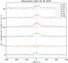 |
Fig. 1 Difference between Hα profile during the flare and quiescence observed on AD Leo. We added a constant (dashed line) to every spectrum that increases with time. The Hα line flux is enhanced, and the profile is asymmetric with the stronger red wing of the line. |
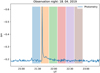 |
Fig. 2 Photometric light curve of the AD Leo flare with marked exposure intervals for the spectra shown in Fig. 1. The light curve is the relative difference in magnitude in the B filter. |
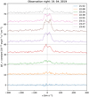 |
Fig. 3 Difference between the Hα profile during the flare and quiescence observed on AD Leo. We added a constant (dashed line) to every spectrum that increases with time. The Hα line flux is enhanced, and the profile is asymmetric with the strong red wing of the line. |
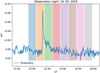 |
Fig. 4 Photometric light curve of the AD Leo flare with marked exposure intervals for the spectra shown in Fig. 3. The light curve is the relative difference in magnitude in the B filter. |
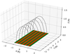 |
Fig. 5 Flare loop arcade structure. Semicircular field lines are shown in black. The green and red stripes mark the stellar surface, and plasma projected onto the stellar surface in a single stripe is assumed to have the same velocity. The coordinates are expressed in the radius of the semicircular field lines. |
3 Model
According to the standard model of solar flares, see, for example, Priest (2014), the energy released during the magnetic reconnection creates a flux of high-energy particles (electrons) that travel along the reconnected magnetic field lines to the lower layers of the solar atmospheres. In the region of higher density, in the chromosphere, these particles transfer their energy to the surrounding plasma by heating it. These regions are bright sources of hard X-ray radiation and are known as flare ribbons. Heated plasma in the chromosphere is pushed down, forming the so-called chromospheric condensation (with velocities of a few dozen km s−1), and simultaneously, the upper chromosphere and low transition region evaporate into the hot loop. These hot loops then cool down and form cool loops that are visible in the Hα line and many other lines of different species (e.g., Mikuła et al. 2017). Downflows in the cool loops have much higher velocities than in the chromospheric condensation, and this also looks consistent with stellar observations. This coronal rain is prominent in Hα and in high-resolution images, and a movie is shown, for example, in Jing et al. (2016). We use this example of an extended flare-loop arcade as a prototype of a stellar case.
In our model, we solved the non-LTE radiative transfer in the Hα line within flare loops that form an arcade-like structure, and we only modeled a situation in which flare loops are already formed. The model was inspired by the coronal rain that occurs on the Sun during solar flares. Our model is based on two assumptions about the general properties of the flare. A flare occurs in the center of the stellar disk with respect to the observer, and the plasma in flare loops moves along the semicircular magnetic field lines in free fall. The arcade structure scheme is shown in Fig. 5.
To solve the radiation transfer through the flare loops, we used the cloud model of plasma (plasma is structured into smaller clouds) with the same physical properties (Tziotziou 2007). These clouds are moving in free fall along the magnetic field lines toward the stellar surface with an initial velocity v0. In this setup, the clouds with the same X coordinate in Fig. 5 (along the arcade) have the same velocity. This is indicated in Fig. 5. The clouds projected onto the stellar surface in the same stripe have the same velocity. The velocity for a given X position can be obtained by solving the Lagrange equations for the Lagrangian,
 (3)
(3)
where g is the surface gravity acceleration of the star, r is the radius of the flare loop along which the cloud is moving, and φ is angle describing the cloud position in Fig. 6. We used the explicit fifth-order Runge-Kutta method to solve the equation with the initial condition φ(0) = 0 and  .
.
Since the clouds have the same physical properties except for the relative velocity toward the stellar surface, we can calculate the spectrum of the arcade as the sum of radiation over the flare area,
 (4)
(4)
where Icloud is the specific intensity of the cloud seen by a static observer with respect to the stellar surface, v is the frequency, τ is the optical thickness of clouds of plasma, υk is the vertical component of the velocity of all clouds in a k-th stripe, Ak is the area of the k-th stripe (area composed of clouds with the same velocity and the same height), and Aflare is the total area of the flare. In our case, it is the area of the whole extended arcade, as discussed by Heinzel & Shibata (2018). The radiation coming from the clouds must be correctly Doppler shifted.
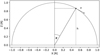 |
Fig. 6 Scheme for the free-fall solution of a cloud of plasma falling along the semicircular magnetic field line. Plane Z = 0 represents the stellar surface. |
3.1 Intensity of a single static cloud
The specific intensity of radiation from a single cloud is given as the solution of the radiative transfer equation,
 (5)
(5)
where S is the source function. The formal solution of the equation is a combination of two terms: the background disk radiation attenuated by the plasma, and the source term of the cloud. The exact formula is
 (6)
(6)
where τ0(v) is the optical thickness of clouds at a given frequency. Assuming optical depth at the line center τ0, we can express τ0(v) = τ0ϕ(v), where ϕ(v) is line profile,
 (7)
(7)
where v0 is the Hα line-center frequency, and Δv is
 (8)
(8)
where T is the plasma temperature, kB is the Boltzmann constant, m is the hydrogen mass, and υt is the turbulent velocity of the plasma. We assumed that the background radiation incoming to clouds, I(v, τ0(v)), is equal to the stellar quiescent radiation without a flare.
We thus need to determine the source function S. For the Hα line, we used a two-level atom approximation, which allowed us to write the source function as the sum of the scattering term and thermal terms (e.g. Heinzel 2019),
 (9)
(9)
where ϵ is the photon destruction probability,  is Planck’s function at the line center frequency with the temperature of the plasma in clouds T, and
  is the mean integrated intensity of the radiation field inside the cloud. Following Rybicki (1984) we can split
  as
as  , where
  is the diffuse part of the intensity, and
  is the part due to direct external illumination of the cloud. Here we present the approximate formula for S that was obtained in a heuristic way by Heinzel & Wollmann (in prep.). Writing formally
 (10)
(10)
we obtain
![Mathematical equation: $S\left( {{\tau _0}/2} \right) = {{{S^{{\rm{dir}}}}\left( {{\tau _0}/2} \right)} \over {1 - \left( {1 - \in } \right)\left[ {1 - {K_2}\left( {{\tau _0}/2} \right)} \right]}},$](/articles/aa/full_html/2023/01/aa44544-22/aa44544-22-eq22.png) (11)
(11)
where K2 is the function evaluated numerically according to Hummer (1982). Its value goes to one for τ approaching zero and decreases with increasing τ. For very small τ, S therefore approaches Sdir, as expected. For optically thin clouds,  is evaluated directly as
 (12)
(12)
where ϕ(v) is the absorption line profile. We can obtain the mean incident radiation intensity simply using the dilution factor W (e.g. Jejčič & Heinzel 2009),
 (13)
(13)
where I(v) is the stellar quiescent specific intensity, and W is
![Mathematical equation: $W = {1 \over 2}\left[ {1 - {{\left( {1 - {{{R^2}} \over {{{\left( {R + H} \right)}^2}}}} \right)}^{{1 \over 2}}}} \right].$](/articles/aa/full_html/2023/01/aa44544-22/aa44544-22-eq26.png) (14)
(14)
R is the stellar radius, and H is the height above the stellar surface. However, for general values of τ, we multiply this direct mean intensity by a correction factor as follows:
 (15)
(15)
This factor goes to one for τ ≪ 1, and we obtain an optically thin value as in Eq. (12). This approach gives a good estimate of the Hα line source function in externally illuminated clouds to within a factor of two. For details and comparisons with exact solutions, see Heinzel & Wollmann (in prep.).
The photon destruction probability ϵ is
 (16)
(16)
 (17)
(17)
where A32 is the Einstein coefficient of spontaneous emission and C32 is the collision coefficient, which can be approximated according to Johnson (1972) as
 (18)
(18)
where ne is the electron density in the clouds, and f(T) is a weak function of the temperature. The values of f(T) for selected temperature values are listed in Table 1.
Since the source function in our approximation is constant inside the cloud, Eq. (6) simplifies to
![Mathematical equation: $I\left( {v,\tau = 0} \right) = I\left( {v,{\tau _0}\left( v \right)} \right){{\rm{e}}^{ - {\tau _0}\left( v \right)}} + {\rm{S}}\left[ {1 - {{\rm{e}}^{ - {\tau _0}\left( v \right)}}} \right].$](/articles/aa/full_html/2023/01/aa44544-22/aa44544-22-eq31.png) (19)
(19)
Value of f(T) for a few selected temperature values.
3.2 Intensity of a single moving cloud
When the cloud is moving with respect to the stellar surface, we need to account for Doppler shifts by modifying both terms in Eq. (19). We calculated the intensity coming from the cloud with the vertical component of the velocity v toward the stellar surface in the reference frame connected to the stellar surface.
The background radiation in the first term is already in the correct frame, so that it does not shift, but is attenuated by the plasma in the cloud that receives the radiation at the shifted (higher) frequency,
 (20)
(20)
where v+ is
 (21)
(21)
The second term represents the radiation coming from the cloud, which must be Doppler shifted to the reference frame; the radiation cloud that emits is seen by the observer at lower frequencies. However, the scattering term in the source function contains background radiation, which for the calculation of  must be shifted as well,
 (22)
(22)
where S(υ) is computed using Eq. (10), but  is due to the Doppler shifts, which are computed as
 (23)
(23)
where v− is
 (24)
(24)
The total intensity observed by the observer is the sum of these two terms:
 (25)
(25)
Using Eq. (4), we can calculate the intensity of the whole arcade.
For the purpose of understanding how the background and source terms affect the final synthetic spectrum, we summed them over the whole arcade like in Eq. (4),
 (26)
(26)
and
 (27)
(27)
3.3 Parameter summary
The model described above has a few parameters, and they are summarized below. We need to know the basic properties of the star on which the loop arcade forms. The parameters that describe the star in our model are the stellar radius R and the quiescent specific intensity Iv. The macroscopic description of the loop arcade requires the radius of the semicircular loops r, the area of the arcade Aflare, and the initial velocity of the plasma clouds at the top of the arcade υ0. To describe the plasma in the clouds, we used the following parameters: the plasma temperature T, the optical thickness of the clouds at the line center τ0, and the turbulent velocity υt in the plasma, which affects the profile width ϕ(v).
4 Results
The results of the modeling described above are presented in this section as the spectra computed for various values of the input parameters. For the quiescent spectrum illuminating the clouds, we used a Gaussian profile that we obtained by fitting the calibrated AD Leo observation in the Hα region plus the continuum fit. In reality, AD Leo Hα does not have a strictly Gaussian shape, but exhibits a reversal in the line core, as shown in Fig. 7. However, to demonstrate the effect of flows on our models, we assumed that a schematic input spectrum will provide basic results; the wing asymmetry is mainly sensitive to the incident radiation outside the central reversal. The Gaussian spectrum we fit is shown in Fig. 7. The stellar radius R for AD Leo we used is 0.39 R⊙ (Reiners et al. 2009).
4.1 Modeled profiles
We modeled Hα line profiles for various input parameters. The results are presented in the following grid of synthetic profiles. One parameter was varied and the others were fixed. We studied the effect of parameters that describe the plasma in our clouds. In the figures below, we plot the synthetic specific intensities calculated using Eq. (4) with the total source term and the total attenuated background term as described above.
The temperature variations for selected parameter values are plotted in Fig. 8. For lower electron density and optical thickness (panels a–d), the source term radiation does not change much with increasing temperature. This is expected as at lower electron densities, the photon destruction probability ϵ is very low, so that the scattering term dominates the source function. For higher electron density (panels e–h), the higher photon destruction probability significantly amplifies the contribution of the thermal term in the source function. The higher optical thickness attenuates the background radiation and also amplifies the source term due to diffusion.
The electron density variations for selected parameter values are plotted in Fig. 9. For a lower temperature and higher optical thickness, panels (a–d) show that the source term is significantly more amplified with increasing electron density. For a higher temperature and lower optical thickness (panels e–h), the source term radiation again increases with increasing electron density. We used the electron densities up to the relatively high 1013 cm−3. These electron densities were recently found in cool flare loops on the Sun (see Jejčič et al. 2018).
The optical thickness variations for selected parameter values are plotted in Fig. 10. For a low temperature (panels a–c), the source term increases strongly, and the attenuated background term decreases with increasing optical thickness.
The turbulent velocity variations for selected parameter values are plotted in Fig. 11. We used relatively hgih values of υt, up to 50 km s−1, which is consistent with the observations of Mikuła et al. (2017). The results of our modeling indicate that an increasing turbulent velocity significantly widens the red wing enhancement for a lower temperature and a higher optical thickness, as well as for a higher temperature and a lower optical thickness.
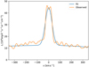 |
Fig. 7 Observed calibrated quiescent spectrum of the AD Leo and the fitted Gaussian profile in the Hα region. This spectrum is used as the background radiation for our model. Compared to the observed AD Leo Hα line, this profile does not feature the small reversal in the line center. |
4.2 Comparison with OES observations
To test the model, we attempted to fit the synthetic profile differences to our OES observations. The data presented in Figs. 1 and 3 are the difference between stellar flux during the flare and the quiescent flux of AD Leo. To calculate the same effect using our model, we computed the flux seen by the observer on Earth, and we subtracted the quiescent radiation we used as the input for our model, expressed as the flux seen on Earth. The flux seen by an observer on Earth under all the assumptions of our model can be approximated as
 (28)
(28)
where  is the synthetic specific intensity calculated using Eq. (4),
  is the quiescent specific intensity of the star, Aflare is the area of the flare, Adisc is the area of the stellar disc, and d is the distance from the star to the Earth. Subtracting the quiescent flux seen by the observer, we obtain the formula
 (29)
(29)
simulating the formula in Eq. (2). During fitting, we varied the model parameters and tried to obtain the best match between the results of the model and the observed Hα line. However, our model does not include any effect that enhances the continuum flux from loops (Heinzel & Shibata 2018), so that an additional constant was included to account for the offset.
For the flare in the Fig. 1, the fit synthetic profile difference is shown in Fig. 12. We fit the spectrum observed on 18 April 2019 at 22:07 UT. The fit parameters are listed in Table 2. The flare area from the fit covers approximately 15% of the stellar disk surface of AD Leo. The observed profile difference has a stronger red wing for velocities within 15–50 km s−1. The synthetic profile difference has a stronger red wing up to velocities of 100 km s−1. Compared to the observed profile difference, the synthetic difference has a similar shape, but appears to be shifted by a few km s−1 toward red velocities.
For the flare in the Fig. 3, the result of our fitting is shown in Fig. 13. We fit the spectrum observed on 19 April 2019 at 23:42 UT. The fit parameters are listed in the Table 2. The flare area from the fit covers approximately 16% of the stellar disk of AD Leo. The observed profile difference has a stronger red wing for velocities within 15–50 km s−1. The synthetic profile difference has a stronger red wing up to velocities of 100 km s−1. Compared to the observed profile difference, the synthetic difference has a similar shape, but appears to be shifted by a few km s−1 toward red velocities, as in the previous comparison.
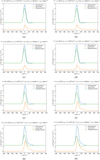 |
Fig. 8 Synthetic Hα line profiles. The modeled specific intensity is the sum of attenuated background radiation and source radiation. The components are plotted as well as the sum. This figure shows variations in the modeled profiles with temperature for two values of the electron density and optical thickness. |
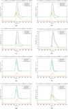 |
Fig. 9 Synthetic Hα line profiles. The modeled specific intensity is the sum of the attenuated background radiation and the source radiation. The components are plotted as well as the sum. This figure shows variations in the modeled profiles with electron density for two values of the temperature and optical thickness. |
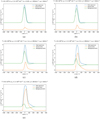 |
Fig. 10 Synthetic Hα line profiles. The modeled specific intensity is the sum of the attenuated background radiation and the source radiation. The components are plotted as well as the sum. This figure shows variations in the modeled profiles with optical thickness. |
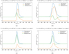 |
Fig. 11 Synthetic Hα line proflies. The modeled specific intensity is the sum of the attenuated background radiation and the source radiation. The components are plotted as well as the sum. This figure shows variations in the modeled profiles with turbulent velocity for two values of the temperature, electron density, and optical thickness. |
Fit model parameter values for the two selected profiles.
5 Discussion
Spectral line asymmetries during stellar flares have been observed for several stars in recent years (e.g., Fuhrmeister et al. 2018; Vida, Krisztián et al. 2019; Leitzinger et al. 2022; Muheki et al. 2020a,b; Koller et al. 2021; Wu et al. 2022). Enhancements of the blue wing of spectral lines are often linked to the possible presence of CMEs. Enhancements in the red wing are associated with downward flows of the plasma, mostly chromospheric condensation or backward-falling material from an eruption, or CMEs that occur close to the limb. The velocities in the red asymmetry can reach several hundred km s−1. Our OES observations of the Hα line indicate velocities up to 50 km s−1, while the observed profile changes are similar to the asymmetries observed by Muheki et al. (2020a).
On the Sun, the observed asymmetries in some spectral lines during impulsive phases of flares are caused by the chromospheric condensation (Kuridze et al. 2015) with velocities reaching a few dozen km s−1. This mechanism might explain some of the lower-velocity red asymmetries observed on M-type stars, but the high-velocity red asymmetries (hundreds of km s−1) suggest other mechanisms to be present. A good candidate seems to be coronal rain, which is a downflow of plasma that usually forms during the gradual phase of flares. It can reach much higher velocities than the chromospheric condensation. Antolin et al. (2010) reported velocities up to 120 km s−1. On cool M-dwarf stars, where flare loops are expected to be much larger than the stellar radius than on the Sun (e.g., Hawley et al. 1995) the velocities of the coronal rain could reach even higher values.
In our model, we solved the Hα radiative transfer inside cool-loop clouds. The synthetic profiles resulting from the whole loop arcade are asymmetrical, with an enhanced red wing of the line. This enhancement can be followed up to 200 km s−1 for the parameters we used. By comparing the synthetic profiles of our model with OES observations, we were able to reproduce a similar shape of the profile with an enhanced red wing, suggesting that coronal rain might create asymmetries that are consistent with observations. However, three discrepancies remained unexplained by our model.
First, the whole synthetic profile difference appears to be somewhat shifted toward the red by a few km s−1. This might be caused by a flare occurring not at the center of the stellar disc, as our model assumes, but rather at a different position. In our model, the flare occurs at the center of the stellar disk with respect to the observer. In this case, all of the clouds in the filled arcade of flare loops move away from the observer. If the flare occurred a little farther from the center of the disc, one half of the clouds close to the top of the arcade would move toward the observer with lower velocities, and the other half of the clouds would move away. The radiation coming from the clouds close to the top moving toward the observer would therefore be blueshifted rather than redshifted. Additionally, some of the clouds close to the far anchor of the flare loops would be covered by the rest of the arcade, and the line-of-sight component of the terminal velocity of the clouds at the other anchor would be lower. This would result in a slightly stronger blue wing and a slightly weaker red wing, virtually shifting the whole profile difference toward blue velocities. If the flare occurred at the limb, most of the clouds would contribute radiation to the blue wing rather than the red one, possibly creating a blue asymmetry. To account for the general location of the flare, a more complex approach is required. This will be a subject of our future studies.
Second, our model does not provide any of the continuum enhancements that are observed by OES. As discussed in Sect. 2, the observed continuum enhancements are caused by the flare and by uncertainties introduced by using linear interpolation during our flux calibration process. To account for this, we just added a constant to the synthetic profile during the fitting. The continuum enhancements are often linked to flare ribbons, which are bright long and narrow areas. However, Heinzel & Shibata (2018) showed that on cool stars, the flare loops can significantly contribute to the total white-light flux. Unlike on the Sun, we are unable to resolve these features on stars. The observed spectra likely contain contributions of both loop and ribbon components, but we assumed that during the gradual phase, the loop arcade dominates. It is well known that in later phases of solar flares, the ribbons fade out while the loops grow and fill an increasingly larger area, e.g. Jing et al. (2016).
Third, the profile differences of the Hα line during the second flare in the Fig. 3 reverse in their center and form a double peak. In our model, we assumed a constant Hα source function in the cloud, which leads by definition to an unreversed profile. The reverted profile can be modeled using the full non-LTE radiative transfer, but this is beyond the scope of this paper and could be the subject of future studies.
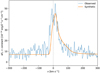 |
Fig. 12 Fit of the modeled spectrum difference ΔFλ and the spectrum difference ΔFλ observed on 18 April 2019 during the gradual phase at 22:07 UT in Fig. 1. To account for the observed continuum enhancements, a constant is added to the synthetic profile difference as a fit parameter. The synthetic profile has a similar shape as the observed profile within the range of 15–50 km s¯1. |
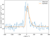 |
Fig. 13 Fit of the modeled spectrum difference ΔFλ and the spectrum difference ΔFλ observed on 19 April 2019 during the gradual phase at 23:42 UT in Fig. 3. To account for the observed continuum enhancements, a constant is added to the synthetic profile difference as a fit parameter. The synthetic profile has a similar shape as the observed profile within the range of 15-50 km s¯1. |
6 Conclusions
We have observed dMe star AD Leo during the spring periods (March and April) in 2019, 2020, and 2021 using the OES attached to the 2-meter Perek telescope at Ondřejov observatory. Simultaneously, in 2019 and 2021, AD Leo photometric observations were carried out. We studied the effect of stellar flares on the Hα line. During flares, we observed that the Hα line exhibited enhancement in the line center and was broadened, and we saw an asymmetry with higher flux in the red wing at velocities within up to 50 km s−1.
In order to explain these Hα profile asymmetries, we developed a simple model based on a direct analogy with solar flares. The model synthesizes Hα profiles emergent from an arcade of flare loops, assuming that the flare occurs at the center of the stellar disc. The resulting Hα profiles are asymmetrical, with an enhanced red wing at velocities reaching up to 200 km s−1.
We attempted to fit the model results to match the observed asymmetries. Our model yields profiles with a similar shape, but the whole profile differences appear to be slightly shifted toward the red by a few km s−1. Moreover, our model does not produce any of the continuum enhancements that OES observed. The whole profile shifting is probably caused by a flare that does not occur at the center of the stellar disc, and thus some contribution from the loop arcade is not redshifted, but can be blueshifted. This effectively shifts the whole profile difference toward the blue wing. More complex geometrical models (projections) must be used to solve this.
Acknowledgements
This study was supported by the Czech Funding Agency grants GACR 19-17102S and 22-30516K, LTT-20015 for data collection with 2-m telescope in 2020 and by RVO:67985815 project. This work was also partially supported by the program “Excellence Initiative - Research University” for years 2020–2026 at University of Wroclaw, project no. BPIDUB.4610.96.2021.KG. This paper is based on the results of the diploma thesis of J. Wollmann. We would like to thank the observers from the SPHE section of the Czech Astronomical Society for providing us with their photometric observations of AD Leo and namely to H. Kučáková for her photometric observations using the Mayer’s telescope at Ondřejov observatory. We are grateful to M. Špoková, R. Karjalainen, J. Šubjak, and M. Skarka for the reduction of spectra from 2-meter Perek telescope and their advice during further processing of spectra and to E. Guenther for his advice during the spectra calibration process. We are also grateful to the referee for his/her useful comments.
References
- Antolin, P., Shibata, K., & Vissers, G. 2010, ApJ, 716, 154 [NASA ADS] [CrossRef] [Google Scholar]
- Crespo-Chacón, I. 2015, PhD thesis, Complutense University of Madrid, Spain [Google Scholar]
- Doyle, L., Ramsay, G., Doyle, J. G., & Wu, K. 2019, MNRAS, 489, 437 [Google Scholar]
- Fuhrmeister, B., Czesla, S., Schmitt, J. H. M. M., et al. 2018, A&A, 615, A14 [NASA ADS] [CrossRef] [EDP Sciences] [Google Scholar]
- Hawley, S. L., Fisher, G. H., Simon, T., et al. 1995, ApJ, 453, 464 [NASA ADS] [CrossRef] [Google Scholar]
- Heinzel, P. 2019, in The Sun as a Guide to Stellar Physics, eds. O. Engvold, J.-C. Vial, & A. Skumanich (Amsterdam: Elsevier), 157 [CrossRef] [Google Scholar]
- Heinzel, P., & Shibata, K. 2018, ApJ, 859, 143 [NASA ADS] [CrossRef] [Google Scholar]
- Hummer, D. G. 1982, J. Quant. Spec. Radiat. Transf., 27, 569 [NASA ADS] [CrossRef] [Google Scholar]
- JejCic, S., & Heinzel, P. 2009, Sol. Phys., 254, 89 [NASA ADS] [CrossRef] [Google Scholar]
- Jejcic, S., Kleint, L., & Heinzel, P. 2018, ApJ, 867, 134 [NASA ADS] [CrossRef] [Google Scholar]
- Jing, J., Xu, Y., Cao, W., et al. 2016, Sci. Rep., 6, 24319 [NASA ADS] [CrossRef] [Google Scholar]
- Johnson, L. C. 1972, ApJ, 174, 227 [NASA ADS] [CrossRef] [Google Scholar]
- Kabáth, P., Skarka, M., Sabotta, S., et al. 2020, PASP, 132, 035002 [CrossRef] [Google Scholar]
- Koller, F., Leitzinger, M., Temmer, M., et al. 2021, A&A, 646, A34 [NASA ADS] [CrossRef] [EDP Sciences] [Google Scholar]
- Kowalski, A. F., Hawley, S. L., Wisniewski, J. R., et al. 2013, ApJS, 207, 15 [NASA ADS] [CrossRef] [Google Scholar]
- Kuhar, M., Krucker, S., Martínez Oliveros, J. C., et al. 2016, ApJ, 816, 6 [Google Scholar]
- Kuridze, D., Mathioudakis, M., Simões, P. J. A., et al. 2015, ApJ, 813, 125 [Google Scholar]
- Leitzinger, M., Odert, P., & Heinzel, P. 2022, MNRAS, 513, 6058 [NASA ADS] [Google Scholar]
- Medina, A. A., Winters, J. G., Irwin, J. M., & Charbonneau, D. 2020, ApJ, 905, 107 [Google Scholar]
- Mikuła, K., Heinzel, P., Liu, W., & Berlicki, A. 2017, ApJ, 845, 30 [CrossRef] [Google Scholar]
- Muheki, P., Guenther, E. W., Mutabazi, T., & Jurua, E. 2020a, A&A, 637, A13 [NASA ADS] [CrossRef] [EDP Sciences] [Google Scholar]
- Muheki, P., Guenther, E. W., Mutabazi, T., & Jurua, E. 2020b, MNRAS, 499, 5047 [NASA ADS] [CrossRef] [Google Scholar]
- Oke, J. B. 1990, AJ, 99, 1621 [Google Scholar]
- Pettersen, B. R. 1989, Sol. Phys., 121, 299 [NASA ADS] [CrossRef] [Google Scholar]
- Pietras, M., Falewicz, R., Siarkowski, M., Bicz, K., & Pres, P. 2022, ApJ, 935, 143 [NASA ADS] [CrossRef] [Google Scholar]
- Priest, E. 2014, Magnetohydrodynamics of the Sun (Cambridge: Cambridge University Press) [Google Scholar]
- Reiners, A., Basri, G., & Browning, M. 2009, ApJ, 692, 538 [NASA ADS] [CrossRef] [Google Scholar]
- Rybicki, G. B. 1984, in Methods in Radiative Transfer (Berlin: Springer), 21 [Google Scholar]
- Shibata, K. 2016, IAU Symp., 320, 3 [NASA ADS] [Google Scholar]
- Švestka, Z. 2007, Sol. Phys., 246, 393 [CrossRef] [Google Scholar]
- Tziotziou, K. 2007, ASP Conf. Ser., 368, 217 [NASA ADS] [Google Scholar]
- Vida, Krisztián, Leitzinger, Martin, Kriskovics, Levente, et al. 2019, A&A, 623, A49 [NASA ADS] [CrossRef] [EDP Sciences] [Google Scholar]
- Wu, Y., Chen, H., Tian, H., et al. 2022, ApJ, 928, 180 [NASA ADS] [CrossRef] [Google Scholar]
All Tables
All Figures
|
Fig. 1 Difference between Hα profile during the flare and quiescence observed on AD Leo. We added a constant (dashed line) to every spectrum that increases with time. The Hα line flux is enhanced, and the profile is asymmetric with the stronger red wing of the line. |
| In the text | |
|
Fig. 2 Photometric light curve of the AD Leo flare with marked exposure intervals for the spectra shown in Fig. 1. The light curve is the relative difference in magnitude in the B filter. |
| In the text | |
|
Fig. 3 Difference between the Hα profile during the flare and quiescence observed on AD Leo. We added a constant (dashed line) to every spectrum that increases with time. The Hα line flux is enhanced, and the profile is asymmetric with the strong red wing of the line. |
| In the text | |
|
Fig. 4 Photometric light curve of the AD Leo flare with marked exposure intervals for the spectra shown in Fig. 3. The light curve is the relative difference in magnitude in the B filter. |
| In the text | |
|
Fig. 5 Flare loop arcade structure. Semicircular field lines are shown in black. The green and red stripes mark the stellar surface, and plasma projected onto the stellar surface in a single stripe is assumed to have the same velocity. The coordinates are expressed in the radius of the semicircular field lines. |
| In the text | |
|
Fig. 6 Scheme for the free-fall solution of a cloud of plasma falling along the semicircular magnetic field line. Plane Z = 0 represents the stellar surface. |
| In the text | |
|
Fig. 7 Observed calibrated quiescent spectrum of the AD Leo and the fitted Gaussian profile in the Hα region. This spectrum is used as the background radiation for our model. Compared to the observed AD Leo Hα line, this profile does not feature the small reversal in the line center. |
| In the text | |
|
Fig. 8 Synthetic Hα line profiles. The modeled specific intensity is the sum of attenuated background radiation and source radiation. The components are plotted as well as the sum. This figure shows variations in the modeled profiles with temperature for two values of the electron density and optical thickness. |
| In the text | |
|
Fig. 9 Synthetic Hα line profiles. The modeled specific intensity is the sum of the attenuated background radiation and the source radiation. The components are plotted as well as the sum. This figure shows variations in the modeled profiles with electron density for two values of the temperature and optical thickness. |
| In the text | |
|
Fig. 10 Synthetic Hα line profiles. The modeled specific intensity is the sum of the attenuated background radiation and the source radiation. The components are plotted as well as the sum. This figure shows variations in the modeled profiles with optical thickness. |
| In the text | |
|
Fig. 11 Synthetic Hα line proflies. The modeled specific intensity is the sum of the attenuated background radiation and the source radiation. The components are plotted as well as the sum. This figure shows variations in the modeled profiles with turbulent velocity for two values of the temperature, electron density, and optical thickness. |
| In the text | |
|
Fig. 12 Fit of the modeled spectrum difference ΔFλ and the spectrum difference ΔFλ observed on 18 April 2019 during the gradual phase at 22:07 UT in Fig. 1. To account for the observed continuum enhancements, a constant is added to the synthetic profile difference as a fit parameter. The synthetic profile has a similar shape as the observed profile within the range of 15–50 km s¯1. |
| In the text | |
|
Fig. 13 Fit of the modeled spectrum difference ΔFλ and the spectrum difference ΔFλ observed on 19 April 2019 during the gradual phase at 23:42 UT in Fig. 3. To account for the observed continuum enhancements, a constant is added to the synthetic profile difference as a fit parameter. The synthetic profile has a similar shape as the observed profile within the range of 15-50 km s¯1. |
| In the text | |
Current usage metrics show cumulative count of Article Views (full-text article views including HTML views, PDF and ePub downloads, according to the available data) and Abstracts Views on Vision4Press platform.
Data correspond to usage on the plateform after 2015. The current usage metrics is available 48-96 hours after online publication and is updated daily on week days.
Initial download of the metrics may take a while.