| Issue |
A&A
Volume 669, January 2023
|
|
|---|---|---|
| Article Number | A156 | |
| Number of page(s) | 11 | |
| Section | The Sun and the Heliosphere | |
| DOI | https://doi.org/10.1051/0004-6361/202244532 | |
| Published online | 26 January 2023 | |
Flares detected in ALMA single-dish images of the Sun
1
Hvar Observatory, Faculty of Geodesy, University of Zagreb, Kačićeva 26, 10000 Zagreb, Croatia
e-mail: This email address is being protected from spambots. You need JavaScript enabled to view it.
2
University of Applied Sciences and Arts Northwestern Switzerland, Bahnhofstrasse 6, 5210 Windisch, Switzerland
3
Institute for Particle Physics and Astrophysics, ETH Zürich, 8093 Zürich, Switzerland
4
Astronomical Institute of the Czech Academy of Sciences, Fričova 298, 25165 Ondřejov, Czech Republic
Received:
18
July
2022
Accepted:
7
November
2022
Abstract
Context. The millimeter and submillimeter radiation of solar flares is poorly understood. Without spatial resolution, millimeter emission cannot be easily compared to flare emission in other wavelengths. Though the Atacama Large Millimeter-submillimeter Array (ALMA) offers sufficient resolution for the first time, ALMA cannot be used on demand to observe when a flare occurs, and when used as an interferometer, its field of view is smaller than an active region.
Aims. We used readily available large-scale single-dish ALMA observations of solar millimeter flares and compared them to well-known features observed in other wavelengths. The properties of these other flare emissions, correlating in space and time, could then be used to interpret the millimeter brightenings and vice versa. The aim is to obtain reliable associations limited by the time and space resolution of single-dish observations.
Methods. Ordinary interferometric ALMA observations require single-dish images of the full Sun for calibration. We collected such observations at 3 mm and 1 mm and searched for millimeter brightenings during times listed in a flare catalog.
Results. All of the flares left a signature in millimeter waves. We found five events with nine or more images that could be used for comparison in time and space. The millimeter brightenings are associated with a variety of flare features in cool (Hα, 304 Å), intermediate (171 Å), and hot (94 Å) lines. In several cases, the millimeter brightening peaked at the footpoint of a hot flare loop. In other cases the peak of the millimeter brightening coincided with the top or footpoint of an active Hα filament. We also found correlations with post-flare loops and the tops of a hot loop. In some images, the millimeter radiation peaked at locations where no feature in the selected lines was found.
Conclusions. The wide field of view provided by the single-dish ALMA observations allowed for a complete overview of the flare activity in millimeter waves for the first time. The associated phenomena often changed in type and location during the flare. The variety of phenomena detected in these millimeter observations may explain the sometimes bewildering behavior of millimeter flare emissions previously observed without spatial resolution.
Key words: Sun: chromosphere / Sun: flares / Sun: filaments, prominences / Sun: radio radiation
© The Authors 2023
 Open Access article, published by EDP Sciences, under the terms of the Creative Commons Attribution License (https://creativecommons.org/licenses/by/4.0), which permits unrestricted use, distribution, and reproduction in any medium, provided the original work is properly cited.
This article is published in open access under the Subscribe-to-Open model. This email address is being protected from spambots. You need JavaScript enabled to view it. to support open access publication.
1. Introduction
Brightenings during solar flares have been reported over the full electromagnetic spectrum, from gamma rays to decameter radio waves (Benz 2017). They are caused by various drivers and mechanisms, but their interpretation remains fragmentary. Little is known about the range from 100 GHz to 10 THz (mid-infrared). In contrast to the flare emission below 100 GHz (Bastian et al. 1998), the spectrum above sometimes increases with frequency, raising the possibility of a “THz-component” (Kaufmann et al. 2004). The millimeter and submillimeter flare observations have been reviewed by Krucker et al. (2013). The > 100 GHz emission correlates best, but not completely, with hard X-rays and gamma rays, sometimes with chromospheric lines. The correlation is often different in the preflare, impulsive, and even post-impulsive phases of a flare as well as in different flares. In one case where the correlation was reliably measured, the position of the 210 GHz emission was associated with two flare ribbons and arcade of loops (Lüthi et al. 2004). Krucker et al. (2013) list ten mechanisms that have been proposed to interpret the THz-component. They remark that there may indeed be more than one explanation.
Interferometric observations using the Berkeley-Illinois-Maryland Array (BIMA) at 86 GHz showed that the millimeter emission of a solar flare exhibits impulsive and gradual phases, which are often both observed in the same flare (Kundu 1996). High spatial resolution images of solar flares at millimeter wavelengths obtained by BIMA showed that most of the gradual phase millimeter flux came from the top of a flaring loop, with some contribution from the footpoints (Silva et al. 1996a,b, 1997; Silva et al. 1998). The millimeter emission from the gradual phase was likely due to thermal bremsstrahlung from the soft X-ray-emitting hot plasma, while gyrosynchrotron radiation was suggested as the main mechanism for the impulsive phase. Raulin et al. (1999) found indications of two different electron populations in the impulsive phase, one responsible for hard X-ray/microwave emission and another for the millimeter emission. Kundu et al. (2000) analyzed two solar flares simultaneously observed at 17, 34, and 86 GHz and reported evidence of bipolar (loop-like) structures.
The major limit of the previous > 100 GHz observations was spatial resolution, which impeded the combination with observations at other wavelengths. The Atacama Large Millimeter-submillimeter Array (ALMA) has a great potential to mitigate this instrumental gap (Wedemeyer et al. 2016; Bastian et al. 2018). Since ALMA is not a solar-dedicated instrument, however, sporadic flares are difficult to observe. For this reason, solar ALMA observations in the past have focused on stationary phenomena, such as radius, center-to-limb, and center-to-pole brightening measurements (Alissandrakis et al. 2017; Selhorst et al. 2019; Sudar et al. 2019a,b; Menezes et al. 2021, 2022); identification and analysis of various stationary structures in full-disk (Brajša et al. 2018; Skokić et al. 2020); and interferometric ALMA images (Iwai et al. 2017; Bastian et al. 2017; Nindos et al. 2018; Jafarzadeh et al. 2019; Rodger et al. 2019; Loukitcheva et al. 2019; Molnar et al. 2019; Shimojo et al. 2020; Wedemeyer et al. 2020; Brajša et al. 2020, 2021).
Recent research extends ALMA results to stationary prominences and filaments (Heinzel et al. 2022; da Silva Santos et al. 2022; Labrosse et al. 2022); dynamical phenomena, such as oscillations in the quiet Sun (Patsourakos et al. 2020; Jafarzadeh et al. 2021; Chai et al. 2022) and transients (Nindos et al. 2020; da Silva Santos et al. 2020; Eklund et al. 2020); and even to submillimeter structures (Alissandrakis et al. 2022). The only known flare-related ALMA observation to date is by Shimizu et al. (2021), who observed an active region with ALMA in interferometric mode at 100 GHz. The field of view was 60″ and the resolution was  . They reported a microflare that correlated in time with Si IV line emission (∼80 000 K) and in space with the footpoint of a soft X-ray loop in the outskirts of the active region.
In this paper, we report on the first solar flares observed by ALMA with complete spatial coverage. The aim of this paper is to analyze the temporal and spatial evolution of five flares observed by ALMA in single-dish mode. We compared images and time profiles with data from other wavelengths to identify counterparts and provide clues for the mechanisms responsible for flare emission at millimeter wavelengths.
2. Data and methodology
Observations of the Sun with the ALMA interferometer require total power full-disk images for absolute calibration (White et al. 2017; Shimojo et al. 2017). These full-disk solar images are publicly available from the ALMA Science Archive1. We limited the data set to ALMA bands 3 (100 GHz, λ = 3 mm) and 6 (240 GHz, λ = 1.2 mm) because other bands were either not public at the time of retrieval or had only a small number of images available. The final data set consisted of 372 images taken between 2016 Dec. 21 and 2019 Apr. 13. They amount to a total on-source observing time of about 40 h. The images were converted to a helioprojective coordinate system and rotated so that the Sun’s north pole pointed upward (Skokić & Brajša 2019). We improved the alignment in all images by limb fitting and double-checking it on compact structures. Next, the images were scaled in intensity so that the brightness temperature of the quiet Sun region nearest the solar center was equal to 7300 K (5900 K) in band 3 (6), as suggested by White et al. (2017). Alissandrakis et al. (2020) reported that in band 6, the value was most probably underestimated by ∼440 K, but we did not include this correction in the present analysis. Finally, the center-to-limb brightness variation was removed by the procedure described in Sudar et al. (2019a).
Depending on the band, it takes ALMA between 10 and 16 min to obtain one full-disk image of the Sun. This is the time the antenna needs to scan the Sun and perform additional calibration scans limiting the maximum cadence. The actual scanning of the Sun without calibration takes 301.4 s in band 3 and 581.4 s in band 6 and thus defines the temporal uncertainty of the images. We transferred the DATE-OBS time in the Flexible Image Transport System (FITS) headers of the ALMA images referring to the beginning of the scan to the middle of the scan.
The observation times of the ALMA images were used to search for coinciding flare events in the Heliophysics Events Knowledgebase (HEK)2. The search returned a list of nearly a hundred entries. However, many of them were related to the same flare event but reported by different observatories or detection methods. These multiple entries were filtered out along with short duration events that occurred between two consecutive ALMA observations and events in which ALMA images were of poor quality due to the presence of scan artifacts or other effects. A total of four flare events were singled out. Additionally, we manually found one event that was visually detected as a small brightening in the ALMA data but was not present in the HEK flare catalog. Details of ALMA observations for all five selected events are listed in Table 1. Flare properties obtained from the HEK catalog are listed in Table 2.
ALMA observation details.
Parameters of the observed flare events retrieved from the HEK database.
The ALMA images were compared with filtergrams in extreme ultraviolet (EUV) from the Atmospheric Imaging Assembly (AIA, Lemen et al. 2012) and magnetograms from the Helioseismic and Magnetic Imager (HMI, Scherrer et al. 2012) on the Solar Dynamics Observatory (SDO, Pesnell et al. 2012). These complementary data were obtained from the Joint Science Operations Center (JSOC)3. We limited the analysis to AIA 94 Å (flaring regions, characteristic temperature of T = 6 × 10⁶ K), 171 Å (quiet corona and upper transition region, T = 6 × 10⁵ K), and 304 Å (chromosphere and transition region, T = 50 000 K). These channels were selected for their characteristic temperature to complement the ALMA data. The HMI data provided photospheric line-of-sight (LoS) magnetic field measurements. We used a cadence of 1 min for AIA images and 45 s for HMI data. Both AIA and HMI data were preprocessed with routines from the Python aiapy software package, which is analogous to the usual SolarSoftWare Interactive Data Language (SSWIDL) aia_prep procedure.
For time profiles, we selected a circular region of a size large enough to cover the entire flaring region and at least the ALMA beam size (∼60″ in band 3 and ∼28″ in band 6). The radius of 100″ was used for the first four flares and 50″ for the SOL2018-12-15 flare. Both the average intensity over this flaring region and the intensity of the brightest pixel in the region were measured at all times in all ALMA and AIA images. The position of peak intensity changes over time and in different wavelengths. While the average intensity is useful for the overall comparison of the ALMA and AIA intensity profiles and estimation of the total energy released, the peak intensity refers to spatially separated individual brightenings and better assesses the maximum increase of the brightness temperature.
The soft X-ray fluxes for all events were observed by the Geostationary Operational Environmental Satellites (GOES), specifically by the GOES-15 X-Ray Sensor (XRS), and were obtained from the National Oceanic and Atmospheric Administration (NOAA). The Hα images are from the Global Oscillations Network Group (GONG) Cerro Tololo Interamerican Observatory in Chile and were taken at the core of the Hα line at 6562.8 Å with a spatial resolution of 1″ per pixel and 1 min cadence. We searched for bursts related to the analyzed flares in dynamic spectra recorded by the solar radio spectrometers e-CALLISTO in the 20−300 MHz range and Radio Solar Telescope Network (RSTN) GHz data, but we found no events.
In the following intensity profile figures, gray-shaded areas indicate the duration of each ALMA scan of the Sun, thus representing time uncertainty of the ALMA measurements. The average intensity of the circular region containing the flare is represented by a black curve while the maximum intensity is depicted as a red curve. The mean ALMA intensity error was obtained from the variation of an intensity profile of a quiet Sun region.
The ALMA images relevant to the flare were further analyzed at the times indicated by vertical blue lines in the intensity profiles. To better isolate the flaring region, a difference image was made by subtracting a reference image. The reference image was usually selected as the ALMA image obtained just before the start of the flare. The effect of solar differential rotation was taken into account. The contours from the ALMA difference image were then overlaid on the HMI magnetogram; the Hα image from the GONG network; and the AIA 304, 171, and 94 Å filtergrams. This was done in order to find counterparts of the ALMA flare emission.
3. Results
3.1. SOL2017-04-23 flare
The SOL2017-04-23 flare is the only ALMA band 6 event in the analyzed set. The advantage of band 6 over band 3 is that it offers twice the spatial resolution of the images, but this is at the expense of temporal resolution, which is decreased due to the longer time required to scan the entire Sun. The beam size is 28.3″ and the pixel size is 3″. ALMA images were produced from PM01 antenna data at 230 GHz (1.3 mm).
The observed ALMA and AIA intensity profiles are shown in Fig. 1 and compared with the GOES XRS flux. The time of the maximum millimeter brightness temperature coincides with the maxima in the other wavelengths. The average ALMA profile and the peak ALMA profile are similar except for the last measurement, where the average rises but the peak values stay constant. The reason for this is an increase in total radiation distributed over a larger area (see the contours at 16:14 UT and 16:34 UT in Fig. 2). The average EUV profiles are similar to each other and to the GOES X-ray curve as well. The peak intensity profiles of the various wavelengths differ more from each other, especially in the 171 Å channel, where many multiple post-maximum peaks can be seen. They indicate strong brightenings originating from small individual areas (high loops).
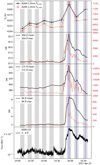 |
Fig. 1. Intensity profiles for the SOL2017-04-23 flare. Gray-shaded areas represent time intervals during which an ALMA image was obtained. Black curves show intensities spatially averaged over the flare region, and red curves show peak intensities within the flare region. The scale of the red curves is given on the right axis in the same units as the black curves given on the left axis. Vertical blue lines denote instants that are shown in cutout images and were further analyzed. The same representation is used in all subsequent intensity profiles. |
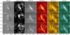 |
Fig. 2. SOL2017-04-23 flare. The ALMA images are difference images between the designated time frame and the base preflare frame. The other are regular full-scale images. ALMA contours outline five levels equidistantly within the range of 100−500 K. The peak ALMA brightness in the flaring region is marked with a white “x”. The intensity was clipped in each image to better show structures of interest. |
The ALMA images of the flaring region are shown in Fig. 2 and compared with HMI LoS magnetograms, GONG Hα images, and AIA filtergrams with overlaid ALMA 100−500 K contours. The Hα and 304 Å images suggest a two-ribbon flare scenario. The first image shown (Fig. 2, 15:57) corresponds to the peak of the flare. The ALMA contours encompass the extent of the flare in Hα, 304 and 94 Å images and coincide with the polarity inversion line in the HMI magnetogram. The peak ALMA brightness in the flaring region, marked with a white “x”, is located near the southern footpoint of a bright 94 Å loop. The ALMA peak is also located near the top of a small loop visible in Hα, 304, and 171 Å.
A second ALMA component, which peaks to the north, coincides with a small filament visible in Hα absorption. The footpoint of a thin loop is visible at the same location in 304 and 171 Å. A third ALMA source with significant brightness is located northwest (up, right) of the main peak. The movies in Hα and 304 Å suggest that the third source is at the location of plasma downflow originating from a region near the second peak.
The next time shown (Fig. 2, 16:14) is around the secondary flare peak visible in 304 and 171 Å average intensity profiles (Fig. 1). The ALMA peak brightness is shifted to the north and next to a small Hα filament that became more pronounced in Hα absorption. The ALMA peak location is consistent with the top of the Hα filament but not with any feature at any other wavelength. However, an intensifying plasma flow can be observed in 304 and 171 Å movies from the main ALMA location, with some of the material falling back to the surface near the location of the second ALMA bright region (on the right).
Finally, in the last ALMA image (Fig. 2, 16:34), the Hα filament has intensified (darkened), and the ALMA contours now correspond well to its shape. The maximum ALMA brightness is situated at the southern footpoint of the filament. The area at the location of plasma inflow (to the right of the filament) has slightly brightened. The original ALMA peak located above the flare ribbons has also brightened and matches the shape of the hot flare loop visible in 94 Å.
We note in the conclusion that the millimeter emission of SOL2017-04-23 is associated with a number of bewildering features: the footpoint of a hot (94 Å) loop (main ALMA peak); the top of cool loops in Hα, 304, and 171 Å; the downflow region in Hα, 304, and 171 Å; and the top and footpoint of a dark Hα filament.
3.2. SOL2017-04-26 flare
The flare that occurred on 2017 Apr. 26 was recorded by ALMA in band 3 in the spectral window centered at 107 GHz (2.8 mm). The beam size is 60″ and pixel size is 6″. Artifacts from the antenna scanning pattern can be seen in ALMA images, especially in the difference images, somewhat affecting the observed shape of the flaring region.
The region-averaged ALMA time profile looks similar to 304 Å, 94 Å, and GOES, but the 171 Å emission peaks significantly later (Fig. 3). The preflare 171 Å average intensity level was even higher than during the flare. This brightness originates from activity within large loops arching over the region. The ALMA peak intensity behaves similarly to the average ALMA intensity. The only difference is that the peak curve maximum occurs before the average maximum, in line with the 304 Å channel behavior.
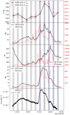 |
Fig. 3. Intensity profiles for the SOL2017-04-26 flare. The colors and markings are the same as in Fig. 1. |
The ALMA peak in the first image at the time of the flare maximum coincides with the bright spot in 94 Å (Fig. 4, 15:32). The region is also bright in Hα and 304 Å images, but not in the 171 Å image. Most 171 Å emission originates from high loops having many small brightenings that do not show in the ALMA image. These brightenings are visible in Hα and 304 Å images and contribute to the high temporal variability at these wavelengths. Whereas the ALMA maximum brightness falls exactly on the 94 Å peak in the flare rise phase, the ALMA peak shifts south along the neutral line in the time steps that follow. The ALMA contours outline the whole flaring region in the next time step (Fig. 4, 15:44). The peak brightness is at the location of the peak in 304 Å. A new thin loop can be seen nearby in 171 Å. The ALMA peak remains in the same place in the next two frames (Fig. 4, 15:56–16:08) where small filamentary structures are forming in 304 Å, while nothing can be seen in 94 Å. However, a secondary ALMA peak is located on two decaying 94 Å flare loops in the northwest.
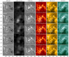 |
Fig. 4. SOL2017-04-26 flare. ALMA contours outline five levels equidistantly in the 50−200 K range. |
As in the case of the SOL2017-04-23 flare, the millimeter emission of the SOL2017-04-26 flare is associated with several different features. We distinguish the footpoint of a hot flare loop in 94 Å, the small 304 and 171 Å brightenings, and the decaying hot loops in 94 Å.
3.3. SOL2018-04-03 flare
The SOL2018-04-03 flare was a short-lived two-ribbon event. The flare lasted less than 20 min, but evolution and post-flare aftermath were well recorded in 23 ALMA images at 95 GHz (3.2 mm). The beam size is 66″ and pixel size is 6″.
The main ALMA peak seems to be delayed in time compared to all other channels. However, this may be the result of undersampling of the ALMA time profile (i.e., missing the peak in millimeter waves). The preflare seen in the ALMA time profile (Fig. 5) coincides in space with a small dark Hα filament (Fig. 6, 14:00). Yet the Hα preflare brightening is related to emissions from the two ribbons located some 28″ to the southeast. Interestingly, there is initially no visible ALMA enhancement around the prominent filament located southeast of the small filament.
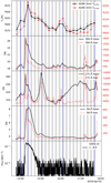 |
Fig. 5. Intensity profiles for the SOL2018-04-03 flare. The colors and markings are the same as in Fig. 1. |
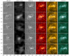 |
Fig. 6. SOL2018-04-03 flare. ALMA contours outline five levels equidistantly in the 50−200 K range. |
At the peak of the ALMA flare (Fig. 6, 14:22), the ALMA maximum moves to the northern footpoint of the larger filament and then also encompasses the flare ribbons and loops visible in 304 and 94 Å. The smaller filament remains enhanced in the ALMA image. The ALMA emission generally follows the neutral line (Fig. 6, 14:22). At the same time, the Hα filament shrank in diameter and length. Further in time, the ALMA peak remains on the larger filament, which becomes more pronounced. The prominent peaks in 171 Å intensity profiles at 15:04 and 17:10 UT are caused by large loops leaving no traces in millimeter waves. The ALMA brightness slightly increases at 16:07 when plasma erupts from the active region and moves south along the major filament, as can be seen in 304 Å movies. Finally, at 17:41 UT, the ALMA intensity peaks near the southern Hα ribbon at a footpoint of a hot loop visible in the 94 Å emission.
The SOL2018-04-03 flare is an example where the ALMA peak emission is best associated with Hα filaments. Filaments are not steadily bright in millimeter emission but become visible due to some activity related to the flare. Millimeter and 94 Å emission are not spatially related except for a microflare in the late post-flare phase.
3.4. SOL2018-04-19 flare
The SOL2018-04-19 flare was spotted while manually browsing ALMA images. The GOES-15 did not detect it in soft X-rays (Fig. 7). Thus, there is no entry for it in the HEK flare catalog. The flare is short and compact and located near the western solar limb where the ALMA antenna scanning pattern smears out sources diagonally. This is clearly visible in the background of Fig. 8.
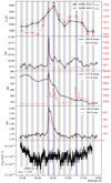 |
Fig. 7. Intensity profiles for the SOL2018-04-19 flare. The colors and markings are the same as in Fig. 1. |
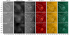 |
Fig. 8. SOL2018-04-19 flare. ALMA contours outline five levels equidistantly in the 50−120 K range. |
The main peak in the EUV lines is sharp and precedes the ALMA peak by around 11 min, although the rise of ALMA intensity is visible even before (see Fig. 7). The ALMA peak coincides in time with a small peak in 304 Å and 171 Å, about 11 min after their main peak. The subpeak is not visible in 94 Å, indicating the absence of hot plasma.
The main ALMA peak is located 25″ southeast of the maxima in the line emissions (Fig. 8, 16:32). The ALMA images show a secondary peak northwest of the main peak. There is no corresponding brightening in the line emissions. This is the case even in the last image when the secondary ALMA peak exceeded in brightness the primary peak (Fig. 8, 17:16).
The SOL2018-04-19 flare is a case where ALMA millimeter waves correlate with cool (Hα and 304 Å) lines, the intermediate 171 Å line, the hot 94 Å line, and the extremely hot bremsstrahlung emission (GOES) in time. However, the main millimeter peak is somewhat displaced in space from the peaks in other wavelengths.
3.5. SOL2018-12-15 flare
The weak SOL2018-12-15 flare occurred close to the limb. ALMA was observing at 95 GHz (3.2 mm). The observed intensity profiles are shown in Fig. 9. The ALMA intensity profile correlates best with 304 Å average intensities but not with the GOES X-ray nor the 94 Å profile, which are similar to each other. The flare reached its peak somewhat earlier in 304 Å relative to the millimeter waves, but much later in 171 Å. The 171 Å emission is dominated by large loops arching over the active region (Fig. 10, 13:58). The averaged profile has a minimum intensity at the time of the ALMA flare peak (13:58 UT) due to dimming of some of the loops.
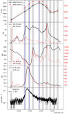 |
Fig. 9. Intensity profiles for the SOL2018-12-15 flare. The colors and markings are the same as in Fig. 1. |
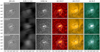 |
Fig. 10. SOL2018-12-15 flare. ALMA contours outline five levels equidistantly in the 50−150 K range. |
As seen in the magnetogram, the brightening in millimeter waves encompasses most of the active region but peaks 25″ farther south where little emission in Hα, 304 Å, 171 Å, and 94 Å originates (Fig. 10, 13:46 and 14:25). Only at the peak time (13:58 UT) of the X-ray and 94 Å intensities does the peak position of all line emissions coincide with the peak in millimeter waves.
The SOL2018-12-15 flare is an example of a weak millimeter emission with little relation to the emission intensity profiles in Hα, 304 Å, 171 Å, 94 Å, and X-rays. The spatial position of the millimeter emission maximum is slightly offset from the bright emission visible in the Hα and EUV lines, except at the time just after the flare peak.
4. Discussion
Significant millimeter radiation was found in all four flares selected from the HEK catalogue. In the event manually selected from ALMA data, associated brightenings are visible in line emission in Hα, 304 Å, 171 Å, and 94 Å. This strongly confirms a general correlation in time between the different radiations originating from very hot, hot, intermediate and cool plasma. The comparison of the images, however, shows a surprising variety of associations with spatial features. A summary of features cospatial with the millimeter emission for each flare is given in Table 3.
Features in other wavelengths coincident with emission in millimeter ALMA images for each flare.
In both ALMA bands 3 and 6, the ALMA flare emission occurs mainly above the neutral line observed in HMI magnetograms. Good examples are Fig. 2 at 15:57, Fig. 4 at 15:44, and Fig. 6 at 14:22. However, this is not always the case, and millimeter emission may correspond to different features, such as Hα active filaments (Fig. 2 at 16:14 and 16:34; Fig. 6 at 14:00, 14:22, and 16:07); 94 Å (hot) loop tops (Fig. 4 at 15:56) or footpoints (Fig. 2 at 15:57); post-flare loops (Fig. 4 at 16:08); or no features in other wavelengths at all (Fig. 8 at 17:16, secondary peak in Fig. 6 at 17:41).
Millimeter emission originating from flaring loop tops and footpoints was previously found at 86 GHz with the BIMA interferometer by Silva et al. (1996b, 1998), who estimated that a major part (around 80%) of the emission in the flare’s gradual phase came from the top of a loop as free-free radiation emitted by hot plasma. Kundu et al. (2000) reported a clear detection of both footpoints of a loop at λ = 3 mm.
Notably, the millimeter flare emission sometimes corresponds very well with filaments, particularly to the activity within them (e.g., SOL2018-04-03). Rutten (2017) predicted that the appearance of the Sun at ALMA wavelengths is expected to be similar to the one in Hα, with good dark-dark correspondence. Brajša et al. (2021) did find dark filaments at 3 millimeters. However, da Silva Santos et al. (2022) found some of the dark threads visible in the AIA 304 Å and Mg II resonance lines to have dark counterparts at 1.25 mm, but their visibility varied significantly across the filament both spatially and temporally. In this paper we report occasional dark (Hα) – bright (mm) correspondence.
Two kinds of time profiles were extracted from the images. The average over the active region, shown with a black solid curve, corresponds to what a low resolution telescope would measure. In a second time profile, represented by a red dashed curve, the peak of the brightest pixel in the area is shown. The second curve indicates small, individual peaks of emission. In all time profiles, the peak pixel curves have both more and shorter maxima than the spatially averaged curves, which indicates that the millimeter flare emission originates from different peaks within the active region. The effect of a multitude of individual peaks is more pronounced in the AIA lines, especially at 171 Å.
The peak pixel intensity measured from the intensity profiles and from the difference ALMA images is given in Table 4. The largest increase is found in the band 6 flare with a value of ΔTb = 563 K above the preflare level, while in band 3 the values vary between 140 and 320 K. This corresponds to 500−1200 K above the quiet Sun level. These values are lower limits since the maximum intensity is spread by the antenna beam for compact, unresolved sources.
NOAA number of the flare active region, peak pixel brightness temperature Tb at wavelength λ, and peak pixel brightness temperature difference ΔTb from the background level.
To statistically investigate the observed similarity of the ALMA and AIA EUV intensity curves, we calculated the Pearson correlation coefficient between ALMA and EUV, average and maximum, time profiles. The results are listed in Table 5. The correlation between the average ALMA profile and the AIA 94 and 304 Å channels is quite good. In three cases, the 304 Å channel, indicating cool plasma, has the highest correlation coefficient. This corresponds to earlier reports about the best spatial correlation with the 304 Å line among all EUV AIA lines (White et al. 2017; Brajša et al. 2018).
Pearson correlation coefficients between intensity measurements from ALMA and different AIA channels.
The 94 Å line, originating from hot plasma, has a slightly higher correlation of the remaining two cases (Table 5). However, the 171 Å line, emitted by plasma of intermittent temperature in coronal loops, has a much lower correlation coefficient, or even an anticorrelation. A similar trend with low 171 Å and high 94 and 304 Å correlations is present in the peak intensity profile. However, there are two exceptions where 171 Å peak emission has a similarly high correlation as 94 and 304 Å channels. The first one is the SOL2017-04-23 flare, where the peak pixel 171 Å curve follows the shape of the ALMA peak and average profiles. The second one is the SOL2018-04-19 flare, where the high 171 Å to ALMA correlation is due to the secondary peak(s).
The observed similarity between 304 Å, 94 Å and ALMA time profiles suggests that the millimeter brightness in flares originates mainly from chromospheric phenomena but occasionally also from hot and dense flare components. Geometry could have a role in the observed correlations as well since the last two flares from Table 5, which have the lowest correlation of the set in 94 and 304 Å lines, are also closest to the solar limb.
The derived contours and locations of maximum intensity are more accurate than the ALMA beam width due to beam oversampling. The confidence interval depends on the statistical significance of the peak above the background and the number of samplings of the single-dish beam, determined by the double-circle scanning pattern. This pattern consists of minor circles with a radius of 600″, whose centers move steadily in a major circle around the center of the Sun at a distance of 600″. Each new minor circle is shifted along the major circle by a defined value called the sampling length (White et al. 2017). In the worst case scenario, the largest distance of the sampled points is less than or equal to the sampling length that has the value of about one-third of the beam width. So the beam is sampled at at least three times the beam resolution, and in many places, such as near the disk center, even more, giving a minimum resolution of 10″ in band 6 and 20″ in band 3. The location of the peak can be determined even more precisely by centroiding.
The flares of this work were not detected in hard X-rays and microwaves. Using the time derivative as a proxy for the hard X-ray flux, we estimated the impulsive phase of the flare by the rise phase of the soft X-rays from the beginning to the peak. In the four flares with significant soft X-rays, the ALMA millimeter intensity is consistent with peaking after the impulsive phase. The SOL2017-04-23 flare (Fig. 1), however, is also consistent with a maximum during the impulsive phase, and the peak intensity curve (red) of the SOL2017-04-26 flare (Fig. 3) clearly has its maximum during the impulsive phase. Thus, > 100 GHz flares appear to be mostly gradual phase phenomena with occasional impulsive phase emission.
5. Conclusions
Full-disk ALMA imaging has yielded the first spatially complete solar flare observations in millimeter wavelengths. The field of view includes the whole disk. We found a field of 250″ × 250″ necessary for a complete overview of the activity taking place in millimeter waves in an active region during a solar flare. It significantly exceeds the field of view of ALMA in interferometric mode. Single-dish observations thus complement interferometric observations in an important way.
Most surprising is the fact that several phenomena in both hot and cold plasma lead to enhanced brightness in millimeter waves. Although there is no evidence contradicting the assumption that the emission process is a thermal free-free emission, it seems that the previous scenario of a chromospheric hot spot heated by a precipitating electron beam is too simplistic.
In addition to footpoints of hot loops, millimeter flare emission was found to be associated with activated Hα filaments, impact points of plasma motions, post-flare loops, and hot loop tops. Surprisingly, we found cases where no feature in Hα, 304 Å, 171 Å, and 94 Å was visible at the position of a millimeter wave emission peak.
In this work, we focused on comparing flare intensity profiles and coincident spatial sources at different wavelengths. More information about the flares, such as temperature and density of the emitting plasma, could be inferred from comparison with simultaneous soft X-ray observations. Such analysis exceeded the scope of this paper but is planned for future work. The detected flares were too small for significant hard X-ray and microwave emissions.
Higher temporal and spatial resolution are needed to gain better insight into the properties of flares at millimeter wavelengths. Both problems can be solved by observing flares using ALMA in interferometric mode; however, this is difficult due to the ALMA scheduling constraints that make it unable to wait for a flare. The field of view in interferometric mode is small, and a lot of luck is needed in order to observe the right location at the right moment. A possible way to achieve better temporal resolution is to use the recently implemented total power regional mapping in single-dish mode. A third possible solution would be to develop more advanced data analysis methods in the future that could go beyond the ALMA full-disk single-dish images presented here. The same data may be better exploited using specific characteristics and redundancies present within them.
Acknowledgments
This work has been supported by the Croatian Science Foundation under the project 7549 “Millimeter and sub-millimeter observations of the solar chromosphere with ALMA”. It has also received funding from the Horizon 2020 project SOLARNET (824135, 2019–2022). This paper makes use of the following ALMA data: ADS/JAO.ALMA#2016.1.01129.S, ADS/JAO.ALMA#2016.1.00070.S, ADS/JAO.ALMA#2017.1.00072.S, ADS/JAO.ALMA#2017.1.01138.S, ADS/JAO.ALMA#2018.1.01879.S. ALMA is a partnership of ESO (representing its member states), NSF (USA) and NINS (Japan), together with NRC (Canada), MOST and ASIAA (Taiwan), and KASI (Republic of Korea), in cooperation with the Republic of Chile. The Joint ALMA Observatory is operated by ESO, AUI/NRAO and NAOJ. SDO/AIA data courtesy of NASA/SDO and the AIA, EVE, and HMI science teams. This work utilizes GONG data obtained by the NSO Integrated Synoptic Program, managed by the National Solar Observatory, which is operated by the Association of Universities for Research in Astronomy (AURA), Inc. under a cooperative agreement with the National Science Foundation and with contribution from the National Oceanic and Atmospheric Administration. The GONG network of instruments is hosted by the Big Bear Solar Observatory, High Altitude Observatory, Learmonth Solar Observatory, Udaipur Solar Observatory, Instituto de Astrofísica de Canarias, and Cerro Tololo Interamerican Observatory. We are grateful to the GOES team for making the data publicly available. We acknowledge the use of the ALMA Solar Ephemeris Generator (Skokić & Brajša 2019). This research used version 3.1.4 (Mumford et al. 2022) of the SunPy open source software package (The SunPy Community 2020). This research used version 0.6.4 of the aiapy open source software package (Barnes et al. 2020). This research made use of Regions, an Astropy package for region handling (Bradley et al. 2022).
References
- Alissandrakis, C. E., Patsourakos, S., Nindos, A., & Bastian, T. S. 2017, A&A, 605, A78 [NASA ADS] [CrossRef] [EDP Sciences] [Google Scholar]
- Alissandrakis, C. E., Nindos, A., Bastian, T. S., & Patsourakos, S. 2020, A&A, 640, A57 [NASA ADS] [CrossRef] [EDP Sciences] [Google Scholar]
- Alissandrakis, C. E., Bastian, T. S., & Nindos, A. 2022, A&A, 661, L4 [NASA ADS] [CrossRef] [EDP Sciences] [Google Scholar]
- Barnes, W. T., Cheung, M. C. M., Bobra, M. G., et al. 2020, J. Open Sour. Softw., 5, 2801 [NASA ADS] [CrossRef] [Google Scholar]
- Bastian, T. S., Benz, A. O., & Gary, D. E. 1998, ARA&A, 36, 131 [Google Scholar]
- Bastian, T. S., Chintzoglou, G., De Pontieu, B., et al. 2017, ApJ, 845, L19 [NASA ADS] [CrossRef] [Google Scholar]
- Bastian, T. S., Bárta, M., Brajša, R., et al. 2018, The Messenger, 171, 25 [NASA ADS] [Google Scholar]
- Benz, A. O. 2017, Liv. Rev. Sol. Phys., 14, 2 [Google Scholar]
- Bradley, L., Deil, C., Patra, S., et al. 2022, https://doi.org/10.5281/zenodo.5826359 [Google Scholar]
- Brajša, R., Sudar, D., Benz, A. O., et al. 2018, A&A, 613, A17 [NASA ADS] [CrossRef] [EDP Sciences] [Google Scholar]
- Brajša, R., Skokić, I., & Sudar, D. 2020, Cent. Eur. Astrophys. Bull., 44, 1 [Google Scholar]
- Brajša, R., Skokić, I., Sudar, D., et al. 2021, A&A, 651, A6 [NASA ADS] [CrossRef] [EDP Sciences] [Google Scholar]
- Chai, Y., Gary, D. E., Reardon, K. P., & Yurchyshyn, V. 2022, ApJ, 924, 100 [NASA ADS] [CrossRef] [Google Scholar]
- da Silva Santos, J. M., de la Cruz Rodríguez, J., Leenaarts, J., et al. 2020, A&A, 634, A56 [NASA ADS] [CrossRef] [EDP Sciences] [Google Scholar]
- da Silva Santos, J. M., White, S. M., Reardon, K., et al. 2022, Front. Astron. Space Sci., 9, 898115 [NASA ADS] [CrossRef] [Google Scholar]
- Eklund, H., Wedemeyer, S., Szydlarski, M., Jafarzadeh, S., & Guevara Gómez, J. C. 2020, A&A, 644, A152 [NASA ADS] [CrossRef] [EDP Sciences] [Google Scholar]
- Heinzel, P., Berlicki, A., Bárta, M., et al. 2022, ApJ, 927, L29 [NASA ADS] [CrossRef] [Google Scholar]
- Iwai, K., Loukitcheva, M., Shimojo, M., Solanki, S. K., & White, S. M. 2017, ApJ, 841, L20 [Google Scholar]
- Jafarzadeh, S., Wedemeyer, S., Szydlarski, M., et al. 2019, A&A, 622, A150 [NASA ADS] [CrossRef] [EDP Sciences] [Google Scholar]
- Jafarzadeh, S., Wedemeyer, S., Fleck, B., et al. 2021, Philos. Trans. R. Soc. London Ser. A, 379, 20200174 [NASA ADS] [Google Scholar]
- Kaufmann, P., Raulin, J.-P., de Castro, C. G. G., et al. 2004, ApJ, 603, L121 [NASA ADS] [CrossRef] [Google Scholar]
- Krucker, S., Giménez de Castro, C. G., Hudson, H. S., et al. 2013, A&ARv, 21, 58 [NASA ADS] [CrossRef] [Google Scholar]
- Kundu, M. R. 1996, Sol. Phys., 169, 389 [NASA ADS] [CrossRef] [Google Scholar]
- Kundu, M. R., White, S. M., Shibasaki, K., & Sakurai, T. 2000, ApJ, 545, 1084 [NASA ADS] [CrossRef] [Google Scholar]
- Labrosse, N., Rodger, A. S., Radziszewski, K., et al. 2022, MNRAS, 513, L30 [NASA ADS] [CrossRef] [Google Scholar]
- Lemen, J. R., Title, A. M., Akin, D. J., et al. 2012, Sol. Phys., 275, 17 [Google Scholar]
- Loukitcheva, M. A., White, S. M., & Solanki, S. K. 2019, ApJ, 877, L26 [Google Scholar]
- Lüthi, T., Lüdi, A., & Magun, A. 2004, A&A, 420, 361 [NASA ADS] [CrossRef] [EDP Sciences] [Google Scholar]
- Menezes, F., Selhorst, C. L., Giménez de Castro, C. G., & Valio, A. 2021, ApJ, 910, 77 [NASA ADS] [CrossRef] [Google Scholar]
- Menezes, F., Selhorst, C. L., Giménez de Castro, C. G., & Valio, A. 2022, MNRAS, 511, 877 [NASA ADS] [CrossRef] [Google Scholar]
- Molnar, M. E., Reardon, K. P., Chai, Y., et al. 2019, ApJ, 881, 99 [Google Scholar]
- Mumford, S. J., Freij, N., Christe, S., et al. 2022, https://doi.org/10.5281/zenodo.6214507 [Google Scholar]
- Nindos, A., Alissandrakis, C. E., Bastian, T. S., et al. 2018, A&A, 619, L6 [NASA ADS] [CrossRef] [EDP Sciences] [Google Scholar]
- Nindos, A., Alissandrakis, C. E., Patsourakos, S., & Bastian, T. S. 2020, A&A, 638, A62 [NASA ADS] [CrossRef] [EDP Sciences] [Google Scholar]
- Patsourakos, S., Alissandrakis, C. E., Nindos, A., & Bastian, T. S. 2020, A&A, 634, A86 [NASA ADS] [CrossRef] [EDP Sciences] [Google Scholar]
- Pesnell, W. D., Thompson, B. J., & Chamberlin, P. C. 2012, Sol. Phys., 275, 3 [Google Scholar]
- Raulin, J. P., White, S. M., Kundu, M. R., Silva, A. V. R., & Shibasaki, K. 1999, ApJ, 522, 547 [NASA ADS] [CrossRef] [Google Scholar]
- Rodger, A. S., Labrosse, N., Wedemeyer, S., et al. 2019, ApJ, 875, 163 [Google Scholar]
- Rutten, R. J. 2017, A&A, 598, A89 [NASA ADS] [CrossRef] [EDP Sciences] [Google Scholar]
- Scherrer, P. H., Schou, J., Bush, R. I., et al. 2012, Sol. Phys., 275, 207 [Google Scholar]
- Selhorst, C. L., Simões, P. J. A., Brajša, R., et al. 2019, ApJ, 871, 45 [NASA ADS] [CrossRef] [Google Scholar]
- Shimizu, T., Shimojo, M., & Abe, M. 2021, ApJ, 922, 113 [NASA ADS] [CrossRef] [Google Scholar]
- Shimojo, M., Bastian, T. S., Hales, A. S., et al. 2017, Sol. Phys., 292, 87 [Google Scholar]
- Shimojo, M., Kawate, T., Okamoto, T. J., et al. 2020, ApJ, 888, L28 [Google Scholar]
- Silva, A. V. R., White, S. M., Lin, R. P., et al. 1996a, ApJS, 106, 621 [NASA ADS] [CrossRef] [Google Scholar]
- Silva, A. V. R., White, S. M., Lin, R. P., et al. 1996b, ApJ, 458, L49 [NASA ADS] [CrossRef] [Google Scholar]
- Silva, A. V. R., Gary, D. E., White, S. M., Lin, R. P., & de Pater, I. 1997, Sol. Phys., 175, 157 [NASA ADS] [CrossRef] [Google Scholar]
- Silva, A. V. R., Lin, R. P., de Pater, I., et al. 1998, Sol. Phys., 183, 389 [NASA ADS] [CrossRef] [Google Scholar]
- Skokić, I., & Brajša, R. 2019, Rudarsko-geološko-naftni zbornik, 34, 59 [CrossRef] [Google Scholar]
- Skokić, I., Sudar, D., & Brajša, R. 2020, Cent. Eur. Astrophys. Bull., 44, 2 [Google Scholar]
- Sudar, D., Brajša, R., Skokić, I., & Benz, A. O. 2019a, Sol. Phys., 294, 163 [NASA ADS] [CrossRef] [Google Scholar]
- Sudar, D., Skokić, I., & Brajša, R. 2019b, Cent. Eur. Astrophys. Bull., 43, 1 [Google Scholar]
- The SunPy Community (Barnes, W. T., et al.) 2020, ApJ, 890, 68 [Google Scholar]
- Wedemeyer, S., Bastian, T., Brajša, R., et al. 2016, Space Sci. Rev., 200, 1 [Google Scholar]
- Wedemeyer, S., Szydlarski, M., Jafarzadeh, S., et al. 2020, A&A, 635, A71 [NASA ADS] [CrossRef] [EDP Sciences] [Google Scholar]
- White, S. M., Iwai, K., Phillips, N. M., et al. 2017, Sol. Phys., 292, 88 [Google Scholar]
All Tables
Features in other wavelengths coincident with emission in millimeter ALMA images for each flare.
NOAA number of the flare active region, peak pixel brightness temperature Tb at wavelength λ, and peak pixel brightness temperature difference ΔTb from the background level.
Pearson correlation coefficients between intensity measurements from ALMA and different AIA channels.
All Figures
|
Fig. 1. Intensity profiles for the SOL2017-04-23 flare. Gray-shaded areas represent time intervals during which an ALMA image was obtained. Black curves show intensities spatially averaged over the flare region, and red curves show peak intensities within the flare region. The scale of the red curves is given on the right axis in the same units as the black curves given on the left axis. Vertical blue lines denote instants that are shown in cutout images and were further analyzed. The same representation is used in all subsequent intensity profiles. |
| In the text | |
|
Fig. 2. SOL2017-04-23 flare. The ALMA images are difference images between the designated time frame and the base preflare frame. The other are regular full-scale images. ALMA contours outline five levels equidistantly within the range of 100−500 K. The peak ALMA brightness in the flaring region is marked with a white “x”. The intensity was clipped in each image to better show structures of interest. |
| In the text | |
|
Fig. 3. Intensity profiles for the SOL2017-04-26 flare. The colors and markings are the same as in Fig. 1. |
| In the text | |
|
Fig. 4. SOL2017-04-26 flare. ALMA contours outline five levels equidistantly in the 50−200 K range. |
| In the text | |
|
Fig. 5. Intensity profiles for the SOL2018-04-03 flare. The colors and markings are the same as in Fig. 1. |
| In the text | |
|
Fig. 6. SOL2018-04-03 flare. ALMA contours outline five levels equidistantly in the 50−200 K range. |
| In the text | |
|
Fig. 7. Intensity profiles for the SOL2018-04-19 flare. The colors and markings are the same as in Fig. 1. |
| In the text | |
|
Fig. 8. SOL2018-04-19 flare. ALMA contours outline five levels equidistantly in the 50−120 K range. |
| In the text | |
|
Fig. 9. Intensity profiles for the SOL2018-12-15 flare. The colors and markings are the same as in Fig. 1. |
| In the text | |
|
Fig. 10. SOL2018-12-15 flare. ALMA contours outline five levels equidistantly in the 50−150 K range. |
| In the text | |
Current usage metrics show cumulative count of Article Views (full-text article views including HTML views, PDF and ePub downloads, according to the available data) and Abstracts Views on Vision4Press platform.
Data correspond to usage on the plateform after 2015. The current usage metrics is available 48-96 hours after online publication and is updated daily on week days.
Initial download of the metrics may take a while.