| Issue |
A&A
Volume 668, December 2022
|
|
|---|---|---|
| Article Number | A43 | |
| Number of page(s) | 14 | |
| Section | Numerical methods and codes | |
| DOI | https://doi.org/10.1051/0004-6361/202244740 | |
| Published online | 02 December 2022 | |
HyperGal: Hyperspectral scene modeling for supernova typing with the SED Machine integral field spectrograph
1
Université de Lyon, Université Claude-Bernard Lyon
1, CNRS/IN2P3, IP2I Lyon,
69622
Villeurbanne, France
e-mail: This email address is being protected from spambots. You need JavaScript enabled to view it.
; This email address is being protected from spambots. You need JavaScript enabled to view it.
2
Division of Physics, Mathematics, and Astronomy, California Institute of Technology,
Pasadena, CA
91125, USA
Received:
11
August
2022
Accepted:
25
September
2022
Abstract
Context. Recent developments in time domain astronomy, such as Zwicky Transient Facility (ZTF), have made it possible to conduct daily scans of the entire visible sky, leading to the discovery of hundreds of new transients every night. Among these detections, 10 to 15 of these objects are supernovae (SNe), which have to be classified prior to cosmological use. The spectral energy distribution machine (SEDM) is a low-resolution (ℛ ~ 100) integral field spectrograph designed, built, and operated with the aim of spectroscopically observing and classifying targets detected by the ZTF main camera.
Aims. As the current pysedm pipeline can only handle isolated point sources, it is limited by contamination when the transient is too close to its host galaxy core. This can lead to an incorrect typing and ultimately bias the cosmological analyses, affecting the homogeneity of the SN sample in terms of local environment properties. We present a new scene modeler to extract the transient spectrum from its structured background, with the aim of improving the typing efficiency of the SEDM.
Methods. HyperGal is a fully chromatic scene modeler that uses archival pre-transient photometric images of the SN environment to generate a hyperspectral model of the host galaxy. It is based on the cigale SED fitter used as a physically-motivated spectral interpolator. The galaxy model, complemented by a point source for the transient and a diffuse background component, is projected onto the SEDM spectro-spatial observation space and adjusted to observations, and the SN spectrum is ultimately extracted from this multi-component model. The full procedure, from scene modeling to transient spectrum extraction and typing, is validated on 5000 simulated cubes built from actual SEDM observations of isolated host galaxies, covering a broad range of observing conditions and scene parameters.
Results. We introduce the contrast, c, as the transient-to-total flux ratio at the SN location, integrated over the ZTF r-band. From estimated contrast distribution of real SEDm observations, we show that HyperGal correctly classifies ~95% of SNe Ia, and up to 99% for contrast c ≳ 0.2, representing more than 90% of the observations. Compared to the standard point-source extraction method (without the hyperspectral galaxy modeling step), HyperGal correctly classifies 20% more SNe Ia between 0.1 < c < 0.6 (50% of the observation conditions), with less than 5% of SN Ia misidentifications. The false-positive rate is less than 2% for c > 0.1 (> 99% of the observations), which represents half as much as the standard extraction method. Assuming a similar contrast distribution for core-collapse SNe, HyperGal classifies 14% additional SNe II and 11% additional SNe Ibc.
Conclusions. HyperGal has proven to be extremely effective in extracting and classifying SNe in the presence of strong contamination by the host galaxy, providing a significant improvement with respect to the single point-source extraction.
Key words: instrumentation: spectrographs / galaxies: general / supernovae: general / methods: data analysis / surveys / techniques: spectroscopic
© J. Lezmy et al. 2022
 Open Access article, published by EDP Sciences, under the terms of the Creative Commons Attribution License (https://creativecommons.org/licenses/by/4.0), which permits unrestricted use, distribution, and reproduction in any medium, provided the original work is properly cited.
This article is published in open access under the Subscribe-to-Open model. This email address is being protected from spambots. You need JavaScript enabled to view it. to support open access publication.
1 Introduction
In the last two decades, time-domain astronomy has become increasingly efficient, thanks to the ability of surveys to conduct (near-) daily scans of the entire visible sky, such as Catalina Real-Time Transient Survey (Drake et al. 2009), PanSTARRS-1 (Kaiser et al. 2002), ASAS-SN (Shappee et al. 2014), and ATLAS (Tonry et al. 2018). A more recent survey is the Zwicky Transient Facility (ZTF, Bellm et al. 2019; Graham et al. 2019), a successor of the Palomar Transient Facility (Law et al. 2009), using a 47 deg2 camera. With such equipment, ZTF can detect O(102) transients of interest every night, with instrumental artifacts and previously known sources excluded, and a typical 5σ r-band AB magnitude limit of 20.5. Among these newly identified sources, 10−15 are new objects that have just appeared and have become bright enough to be detected. Once the photometric detection is triggered, ZTF relays the alert to the Spectral Energy Distribution Machine (SEDM, Blagorodnova et al. 2018), an integral field spectrograph (IFS), designed and built to spectroscopically classify transients brighter than ~19.5 mag, operating on the Palomar 60-in. telescope. The core of the SEDm is a Micro-Lenslet Array (MLA) covering 28″ × 28″, subdivided into 52 × 45 hexagonal spaxels, combined to a multi-band (ugri) field acquisition camera, used for positioning and guiding.
Currently, the automated pipeline routinely used for IFS data reduction and supernova (SN) spectrum extraction is pysedm (Rigault et al. 2019). Since this pipeline intrinsically assumes the target is an isolated point source, it cannot properly handle the situation where the transient is close to its host galaxy core. As a matter of fact, since August 2018, some 30% of the observed SNe exhibit some severe host contamination, which significantly decreases the confidence level of the classification, and about 10% are simply unusable. This situation has various undesirable effects. From a mere statistical point of view, discarding SNe with too strong a host contamination reduces the type la SN (SN la) sample by 10–20%, which weakens the strength of the Hubble diagram anchor at low redshift. Furthermore, the wrong classification of SNe la could induce a significant bias in the cosmological analysis (e.g., Jones et al. 2017).
Finally, a more subtle effect is related to the galactic environment bias, which would be caused by extracting host-contaminated SNe (Rigault et al. 2013). In recent years, numerous studies have shown that the SN la standardized luminosity is tightly correlated with environmental properties. Rigault et al. (2015, 2020) showed that, after standardization for light curve shape and color, SNe la characterized by a high local specific star formation rate (IsSFR) are fainter by 0.16 ± 0.03 mag. Other tracers, such as host galaxy stellar mass (Kelly et al. 2010; Sullivan et al. 2010; Childress et al. 2013; Betoule et al. 2014) or simply host morphology (Pruzhinskaya et al. 2020), are finding the same correlation between SN la luminosity and their environment. Recently, Briday et al. (2022) showed that all these tracers are compatible with two SN la populations differing in standardized magnitude by at least 0.12 ± 0.01 mag.
Some developments have been made to improve the robustness of the point source extraction by estimating the faintest iso-magnitude contour separating the galaxy and the SN (Kim et al. 2022); however, this is not yet an optimal solution in most problematic situations; for instance, when the SN is faint or located near the host core, it only brings a marginal 1.7% improvement in classification accuracy from the standard pysedm analysis.
We might consider handling the host contamination by interpolating the galaxy area under the transient from the external parts in the field of view (FoV). Unfortunately, there are several reasons for not using such a method, beyond the mere signal-to-noise issue. First, there is the seeing, which makes the SN spread over the galaxy structure: as much as the host light is contaminating the SN flux, the reverse is also true, and it is not clear how far from the SN position we would consider the galaxy flux to be free of the point source signal. Furthermore, the host spatial structure under the SN extent – linear, concave, or convex – is not known a priori, especially in a strongly structured region such as the galaxy core, which would prevent a clean and robust interpolation. Finally, an interpolation would assume that the host spectral features are spatially uniform under the SN extent, which again is usually not the case, especially close to the galaxy core.
In order to improve the final SN la sample in as many ways as possible, we look to HyperGal1, a scene modeler specifically designed to handle the strong host contamination case through a detailed hyperspectral galaxy modeling, complemented by a smooth background component and a point-source transient. The algorithm concept is based on two ideas: first, public multi-band wide photometric surveys can provide reference information on the host galaxy before the transient event; second, the required host galaxy cube (two spatial dimensions and one spectral one) can be estimated from pure photometric observations using a dedicated SED fitter as a physically motivated spectral interpolator. The resulting hyperspectral host model can then be projected in the observable space of the SEDM, taking into account all observational effects: relative geometry between the photometric pixels (px) and the IFS spaxels (spx), spatial (point spread function, PSF) and spectral (line spread function, LSF) impulse response functions (IRF) of the SEDM, atmospheric differential refraction (ADR), sky background, and additional diffused light.
In Sect. 2, we describe the HyperGal pipeline and the validation tests on realistic simulations are presented in Sect. 3 to estimate the accuracy of the SN extraction as well as the SN typing itself, since this is what the SEDM is designed for. We also show the improvement with respect to an isolated source extractor such as pysedm. A discussion of the relevant hypotheses and possible future improvements are given in Sect. 4.
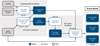 |
Fig. 1 Main processing steps of the HyperGal pipeline and sections where they are detailed. |
2 HyperGal pipeline
This section presents the different processing steps from the required input to the transient spectrum extraction (Fig. 1). The supernova ZTF20aamifit, at a redshift of z = 0.045 as measured from strong Hα line in the host spectrum, is systematically used here for illustration. It was observed with the SEDM in February 17, 2020, at airmass 1.7 in poor seeing conditions (274 FWHM). It is ~2″./8 away from its host galaxy core, close enough to not be considered as isolated (see Fig. 2).
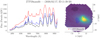 |
Fig. 2 SEDM cube from the observation of ZTF20aamifit. Left panel shows the spectra, whose color corresponds to the selected spaxels in the right panel (white image of the spectrally integrated cube). Red cross shows the SN position. |
2.1 Inputs
Three main inputs are necessary to run HyperGal: the SEDM cube to be analysed, the archival photometric thumbnails, and the redshift of the target. The SEDM IFS (x,y,λ) cube of the scene is built from the 2D raw spectroscopic exposures with pysedm (Rigault et al. 2019, Sect. 2). It includes all the components, such as the transient point source, spatially and spectrally structured host galaxy, night sky background, and spatially smooth diffused light, to be handled by the scene modeler (Fig. 2).
The archival multi-band photometric images of the transient environment, acquired before the SN explosion, are obtained from the PanSTARRS-1 (PS1) 3π Steradian survey (Chambers et al. 2016) in all grizy bands and queried at the SN location through the Image Cutout Server2. In particular, PS1 was chosen for its sky coverage compatible with ZTF (north of declination −30 deg). Figure 3 shows an RGB image for ZTF20aamifit host galaxy through the PS1 grz bands.
An analysis of spatially structured scenes (harboring three or more well-resolved objects in the SEDM FoV) provides a precise estimation of a scale ratio of SEDM and PS 1 pixel sizes of 2.230 ± 0.003, which, for a PS1 px scale of 0″.25, corresponds to an effective SEDM spaxel size of 07558. Once measured, this SEDM scale is fixed in the pipeline. To save computation time for the SED fit and the spatial projection step, PS 1 images were first spatially rebinned following 2×2.
The third input is the host galaxy redshift, required by the SED-based interpolation of the photometric images. Around 50% of the targets observed by the SEDM have a host galaxy spectroscopic redshift known beforehand (Fremling et al. 2020); for the others, a redshift is a priori estimated from a preliminary transient spectrum extraction, using the transient spectral features and the possible presence of emission lines from the host galaxy. While it would be theoretically possible to assess the host redshift directly during the scene modeling, we did not try to implement this feature yet (see Sect. 4). Furthermore, the consequences of an inaccurate input redshift are not considered in this analysis.
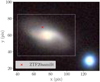 |
Fig. 3 RGB image of the host galaxy of SN ZTF20aamifit, constructed from the PS1 grz cutouts. The red cross shows the position of the SN detected by ZTF. The x- and y-axes are in native PS1 pixels, 0725 aside. White dashed box is used as the boundaries in Figs. 4 and 6. |
2.2 SED fit
The SED fit aims to generate an effective hyperspectral, namely a full 3D (x, y, λ), host model from the grizy PS 1 broadband images. During the process, each photometric pixel is treated independently, so that the resulting spaxel in the output cube gets its own spectrum. At the end of this process, this cube is still independent of the SEDM observation details (impulse responses, atmospheric effects, etc.). It is important to note that the SED fitter is not used here to derive accurate and spatially resolved physical parameters from the host galaxy, but rather to build a physically plausible spectral interpolation compatible with broadband archival images.
The software used for this step is cigale3 (Burgarella et al. 2005; Noll et al. 2009; Boquien et al. 2019). It is based on a progressive computation, successively using modules describing a unique component of the SED. The set of all parameters tested by cigale is shown in Table 1.
2.2.1 Star formation history and population
The time-evolution of the star formation rate (SFR) is described by the star formation history (SFH) through the sfhdelayed module. Our SFH scenario includes two components: a delayed SFR and a late burst:
 (1)
(1)
Both terms have a decreasing exponential form:
 (2)
(2)
 (3)
(3)
The amplitude of the late starburst is fixed by the parameter fburst, defined as the ratio between the stellar mass formed during this event and the total stellar mass. The SFH is applied with the initial mass function (IMF) from Chabrier (2003) on the stellar population model from Bruzual & Chariot (2003), used through the be⍉3 module.
Modules and input parameters used with cigale.
2.2.2 Nebular emission
The light emitted in the Lyman continuum by the heaviest stars ionizes the gas in the galaxy. This physical process generates significant radiative emission in the continuum and spectral lines. This SED component is described by the nebular module, based on Inoue (2011). The model is effectively parameterized by the metallicity Z (the same as in the stellar population model bc⍉3) and the ionization parameter log(U).
2.2.3 Dust extinction
Dust in the galaxy absorbs the radiation at short wavelengths, especially from the UV to the near-IR; this energy is then reemitted in the mid- to far IR. As HyperGal is primarily targeting sources at redshift z < 0.1 in the optical domain, the extinction effect is properly considered through the dust attenuation module dustatt_modified_CF⍉⍉ from Charlot & Fall (2000). This approach is considering two star populations: the young ones (<107 yr) still reside in their birth cloud (BC), and the old ones are considered as already dispersed in the interstellar medium (ISM). Attenuation is therefore treated differently: for the young population, both ISM and BC are considered, while for the old population, only the ISM is considered. In both case, the attenuation Aλ is modeled by a power law, normalized by the V-band attenuation:
 (4)
(4)
with λV = 0.5 µm. The young-to-old star V-band attenuation ratio is parameterized through  , a free parameter allowing for more flexibility and a better estimate of the Hα emission lines (Battisti et al. 2016; Buat et al. 2018; Malek et al. 2018; Chevallard et al. 2019). The power-law slope for the ISM is fixed at nISM = −0.7 following Charlot & Fall (2000), and the slope for the BC at nBC = −1.3 as advocated in da Cunha et al. (2008). For completeness, the dale 2014 module was used for the dust emission (Dale et al. 2014); however, this complex component has no significant impact in our spectral domain.
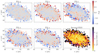 |
Fig. 4 Map of the pull for the grizy broadband images from cigale outputs, and spectral relative rms over the five reference host images, shown from left to right and top to bottom. Only pixels with S/N > 3 for all grizy bands are considered (see Sect. 2.2). |
2.2.4 From SED fit to hyperspectral galaxy model
We ran cigale using PS1 filter transmission curves from (Tonry et al. 2012, see Fig. 6) on photometric pixels for which the signal-to-noise ratio (S/N) is above 3 in all 5 bands. Otherwise, the output flux is set to 0 at all wavelengths: such pixels presumably belong to the sky or diffuse backgrounds and cannot be properly modeled by the SED fitter. For all fitted pixels, cigale returns a spectrum over an extended wavelength domain (from far UV to radio), with an inhomogeneous spectral sampling between 1 and 5 Å px−1. All spectra are rebinned at the SEDM spectral sampling of ~26 Å px−1 and truncated to the [3700, 9300] A range, resulting in 220 monochromatic slices.
The broadband flux from the SED fit is compared to the input photometric measurements in Fig. 4, where we show for each PS1 band and pixel, the pull (i.e., the model residual normalized by the error on the data) and the relative rms averaged over the five bands:
 (5)
(5)
where fλ denotes the data and  the predicted value. The averaged rms is generally lower than 3% in the core of the galaxy, but can reach ~10% in the outer parts. However, as the PS1 observations are 2–3 magnitude deeper than the SEDM ones (Chambers et al. 2016), relatively poorly fitted pixels far away from the host core have a marginal flux impact proportionate to the SEDM background and, thus, they do not significantly affect the transient spectrum in the scene model.
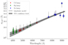 |
Fig. 5 LSF standard deviation, σLSF, as a function of wavelength, from the wavelength calibration of 65 nights between 2018 and 2022. Each violin corresponds to an emission line in the arc-lamp spectra (color legend). |
2.3 SEDM impulse response functions
At the next step, the “intrinsic” hyperspectral galaxy model obtained from the SED fit has to be projected in the SEDM observation space, including the spectro-spatial IRFs. This section first presents the spectral component, namely, the line spread function (LSF), then the spatial component, known as the point spread function (PSF).
2.3.1 Spectral IRF (LSF)
The output spectra from cigale have a spectral resolution of ~3 Å in the wavelength range 320029500 Å (i.e., a median resolving power of ℛ = λ/Δλ ~ 2000, Bruzual & Charlot 2003), which is 20 times the near-constant SEDM resolution (ℛ ~ 100, Blagorodnova et al. 2018). The full SEDM LSF is therefore a very good approximation of the differential spectral IRF between cigale and the SEDM. To characterize the SEDM LSF, we used the intermediate line fits of the wavelength solution derived from arc-lamp observations, Cd, Hg, and Xe (Rigault et al. 2019, Sect. 2.1.2). Each emission line was fit by a single Gaussian profile over a third-order polynomial continuum.
Studying wavelength calibration for 65 nights between 2018 and 2022, the LSF standard deviation σLSF turned out to be stationary (no evidence of evolution with time) and fairly homogeneous in the FoV, but chromatic (as expected). Figure 5 shows the chromatic evolution of the standard deviation, and the quadratic polynomial model adjusted to it.
To adapt the cigale spectra to the SEDM resolution, the spectra of the hyperspectral galaxy model were convolved by the chromatic Gaussian LSF. An illustration of the result is shown in Fig. 6.
2.3.2 Spatial IRF (PSF)
The SNe are effective point sources, thus, they can be solely described in the FoV by the SEDM PSF (and its amplitude). HyperGal uses a bisymmetric PSF model, in which the radial profile is the sum of a Gaussian N(r; σ) for the core, and a Moffat ℳ(r; α,β) for the wings (Buton et al. 2013; Rubin et al. 2022):
 (6)
(6)
where r is an elliptical radius:
 (7)
(7)
with (x0, y0) the coordinates of the point source. Parameters A and ℬ simultaneously describe the flattening and the orientation of the PSF.
The four shape parameters (α,β,σ,η), which could be ill-constrained in low S/N regime if adjusted independently, are correlated by fixed relationships. The PSF was tested on 148 isolated standard stars, observed in 2021 with the SEDM, and we settled on the following model. The constrained PSF only has two free parameters: α (Moffat radius) and η (relative normalization of the Gaussian), while the two other parameters are expressed as linear functions of α:
 (8)
(8)
 (9)
(9)
where β0 = 1.53, β1 = 0.22, σ0 = 0.42, and σ1 = 0.39 were determined from the training star sample.
The chromaticity of α(λ) is set as a power law function:
 (10)
(10)
where normalization αref and index ρ are free parameters, and λref ≡ 6000 Å. Parameters η, A, and ℬ do not exhibit strong chromaticity and are therefore considered constant. Finally, the SEDM PSF of a given observation is fully described by five independent parameters: αref and ρ, η, A, and ℬ.
2.3.3 Differential PSF between PS1 and SEDM
The original hyperspectral galaxy model is derived from PS1 photometric exposures, with different seeing conditions than the SEDM observations: the median seeing is ~1″.7 in SEDM (Blagorodnova et al. 2018), and ~1″.2 in PS1 images (Waters et al. 2020).
As the exact PSF profile is less critical for extended objects such as the host galaxy, we chose to model the differential PSF between PS1 and SEDM as a single bisymmetric Gaussian kernel, with free ellipticity and position angle. The hyperspectral model is thus convolved with this differential PSF before the spatial projection.
2.4 Scene modeling
At this point, we have the two main elements on hand to build the scene model: 1) a hyperspectral host galaxy model, as well as the (differential) spectral and spatial IRF to match it to the SEDM observations; 2) a chromatic PSF model for the transient point source. The last component needed to complete the scene is the night sky and diffused light background, modeled with a 2D 2nd-order polynomial at each wavelength. The nonuniform terms handle a strong diffused light component, clearly visible in the edges of the SEDM FoV and spectral range. Overall, the background component is described by six parameters: b0, bx, by, bxy, bxx, and byy. We go on to describe the progressive method used to adjust it to the observed SEDM cube as well as the detailed spatial projection procedure used to match the two cubes.
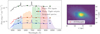 |
Fig. 6 Hyperspectral galaxy model of ZTF20aamifit host galaxy, after projection in the SEDM observation space (including LSF). Green circles correspond to the spatially integrated flux from PS1 cutouts, while black diamonds refer to the same quantities as fit by cigale. The five shaded curves show the transmission of the grizy PS1 filters. Red and blue spectra on the left correspond to the spectra integrated in selected regions of same color in the model cube on the right. The black spectrum is the spectrum integrated over the full FoV. |
2.4.1 General method
We first considered N ≪ 220 “meta” slices of the SEDM cubes, that is, slices summed over a restricted wavelength domain that are small enough to be considered roughly achromatic, but large enough to increase the S/N and significantly speed up the computation time. The scene is projected and fitted on all metaslices independently (the so-called “2D fit”; Sect. 2.4.3), which results in a set of N × m parameters; some are nuisance parameters (e.g., background and component amplitudes), other key scene parameters, such as the point source position, and PSF shape parameters.
From this set of parameters evaluated at N wavelengths, specific chromatic models were used to fix all shape and position quantities (the “1D fit”), for which the full spectral resolution is not required. Ultimately, HyperGal performs a final linear “3D” fit of the different component amplitudes over all monochromatic slices, providing the total scene model cube at original SEDM spectral sampling.
The pipeline uses by default N = 6 metaslices linearly sampled between 5000 and 8500 Å. This spectral range is where the SEDM efficiency is higher than 70% (Blagorodnova et al. 2018) and is extended enough to well constrain the chromatic parameters, especially the ADR (see Sect. 2.4.4). The pipeline was tested with different number of metaslices, but no significant difference was noticed in the results.
HyperGal was extensively optimized with the parallel computing library DASK4 (Dask Development Team 2016), a dynamic task scheduler working as well on single desktop machines as on many-node clusters. DASK optimizes the pipeline by analyzing the (minimal) interdependencies between all computation tasks and building an optimal parallelized workflow to be submitted and run on an arbitrary number of available workers (in our case, we used ten nodes on the IN2P3 Computing Center5).
2.4.2 Spatial projection
The spatial projection of the hyperspectral galaxy model (matched to the SEDM spectral and spatial IRFs) was done by successively projecting each (meta)slice, taking into account the relative geometry and size between PSl-derived model (square, 0″.50 aside) and SEDM (hexagonal, 0″.558) spaxels. The projection is based on a spatial anchor, that is, a reference position in the sky supposedly known in both (meta)slices. The chosen anchor is the transient position, derived from the ZTF survey astrometry and located at the center of the queried PS1 images (and therefore at the center of the hyperspectral model). In the SEDM cube, this position is initially guessed from the astro-metric solution of the SEDM Rainbow Camera (Blagorodnova et al. 2018; Rigault et al. 2019), but cannot be strictly fixed: the (chromatic) SEDM anchor position (x0, y0) is free in the fitting process of each metaslice. The projection is done by geometrically overlapping the two polygonal spaxel grids, with the anchor position as a reference; this is effectively equivalent to a nearest neighbor interpolation scheme. These computations were done using shapely6 (Gillies et al. 2007) and geopandas7 (Jordahl 2014). At this point, the model cube which the PS1/SEDM differential PSF and the SEDM LSF were applied to is now projected in the SEDM observation space, over the SEDM spaxel grid.
2.4.3 Metaslice (2D) fit
As already mentioned, all components of the scene are first independently fitted on the N metaslices. The free parameters per metaslice are: (1) the SN position (x0, y0) in the SEDM FoV, used as an anchor position for the spatial projection; (2) the SN PSF parameters (α, η, A, ℬ); (3) the PS1/SEDM differential PSF parameters (σG, AG, ℬG); (4) the amplitudes of the SN (I) and host (G) components; (5) the background coefficients (b0,bx,by,bxy,bxx,byy). We used iminuit8 (James & Roos 1975; Dembinski et al. 2020) to minimize a weighted χ2 for each metaslice independently:
 (11)
(11)
where i runs on the spaxels of the metaslice, y and  are the data and model fluxes respectively, and σ is the error on the data.
Figure 7 illustrates the projection of one metaslice of the hyperspectral galaxy model onto the SEDM space. The fitted scene on this metaslice shows a spatial rms between the model and the data of 2.6%. Although indicative of the overall scene model accuracy, a low rms does not necessarily imply a clean separation of the different components, (e.g., when the transient lies on top of a sharp host galaxy core). Extraction accuracy is directly evaluated from simulated SN spectra in Sect. 3.
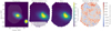 |
Fig. 7 Fit result for the [6167, 6755] Å metaslice of ZTF20aamifit cube. From left to right: metaslice from the original (transient-free) hyperspectral model with MLA footprint overplotted, projected fitted scene (host + background + SN), SEDM observations, and relative model residuals. |
2.4.4 Chromatic (1D) fit
Once the fit is performed independently overall N metaslices, a set of N chromatic estimates of the m parameters is at hand to assess their (smooth) chromatic evolution − except for the component amplitudes and background parameters, which are nuisance parameters at this point.
The chromaticity of the full Gaussian + Moffat PSF is modeled as described in Sect. 2.3.2. The chromaticity of the width of the 2D Gaussian which models the differential PSF between PS 1 and the SEDM is adjusted by a similar power law:
 (12)
(12)
where ρG and σref are adjusted on the N metaslice estimates obtained previously, and λref ≡ 6000 Å; the shape parameters AG and ℬG are considered constant equal to their (inverse-variance weighted) mean values over the N metaslices.
The effective anchor location in the SEDM FoV is systematically wavelength-dependent, due to the chromatic light refraction through the atmosphere (ADR). Given the N positions of the SN in the different metaslices, an effective four-parameter ADR can be fitted to track the chromatic offsets in the FoV:
![Mathematical equation: $\left[ {\matrix{ {{x_0}\left( \lambda \right)} \hfill \cr {{y_0}\left( \lambda \right)} \hfill \cr } } \right] = \left[ {\matrix{ {{x_{{\rm{ref}}}}} \hfill \cr {{y_{{\rm{ref}}}}} \hfill \cr } } \right] - {1 \over 2}\left( {{1 \over {{n^2}\left( \lambda \right)}} - {1 \over {{n^2}\left( {{\lambda _{{\rm{ref}}}}} \right)}}} \right) \times \tan \left( {{d_z}} \right)\left[ {\matrix{ {\sin \theta } \hfill \cr {\cos \theta } \hfill \cr } } \right],$](/articles/aa/full_html/2022/12/aa44740-22/aa44740-22-eq18.png) (13)
(13)
with (θ, z, xref, yref) the fitted parameters, where θ is the parallactic angle, z is the airmass and dz = arccos z−1 is the zenith distance in the plane-parallel atmosphere approximation, and (xref, yref) is the reference position at reference wavelength λref ≡ 6000 Å. The index of refraction n(λ) of air is computed using the Edlén equation from Stone & Zimmerman (2001)9, which takes into account the atmospheric pressure, temperature, and relative humidity, as provided for each exposure by the SEDM Telescope Control System.
Figure 8 illustrates the ADR effect, a drift of the metaslice anchor position with wavelength and the ADR model at an effective airmass of ~2.0.
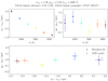 |
Fig. 8 SN positions as a function of wavelength, and the effective ADR fit. Top panel: relative offsets with respect to reference position at reference wavelength along each axis; filled points correspond to the observed offsets, and open circles to the predictions of the ADR model. Bottom panel: relative offsets in the (x, y) plane. Color codes refer to the central wavelength of the metaslices. |
2.4.5 Final (3D) fit
Once all PSF and ADR chromatic models are available from 2D + ID metaslice adjustments, the scene morphological parameters are considered known and fixed at each wavelength: the point source position (x0,y0) and PSF parameters (α, η, A, ℬ), as well as the PS1/SEDM differential PSF parameters (σG, AG, ℬG). This allows us to perform a final 3D linear fit over all monochromatic slices, where only scaling amplitudes of the different scene components − namely, host galaxy {G}, SN {I} and background polynomial components {b0,bx,by,bxy,bxx,byy} – are let free per slice. The total scene is then reconstructed at the full spectral resolution.
Although G(λ) is primarily used to recover flux calibration mismatch between PS 1 and SEDM, this normalization parameter can interfere in a nontrivial way with the position and intensity of the emission lines in the hyperspectral galaxy model. This effect might help in handling slightly incorrect input redshift used in the SED fitting step, especially under the assumption of a uniform spatial distribution of the line. As this has not been analysed in depth, we elaborate on this notion in Sect. 4.
Figure 9 presents the white image (spectral integral) of the final HyperGal scene model for SN ZTF20aamifit. The quality of the fit is evaluated from the pull map, showing no evidence of structured residuals. The spectral relative rms map indicates an accuracy of ~4% at SN and host core location, and 6–7% where only the background is significant.
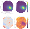 |
Fig. 9 Full scene model for ZTF20aamifit. Top panel: integrated SEDM and HyperGal-modeled cubes; the red cross indicates the adjusted point source position at 6000 A. Bottom panel: spectral pull and spectral relative rms. No galaxy- or SN-related structured residual is visible in the pull map and the spectral rms indicates an accuracy of ~4% at the host and SN locations. |
2.5 Component extraction
The strength of the HyperGal pipeline is the simultaneous fit of the 3 scene components, the host galaxy, the transient point source and the background. The main quantity of interest is of course the SN spectrum (i.e., the vector of the point source amplitudes I(λ), see Fig. 10), but we can also selectively subtract individual components to assess the quality of the scene model.
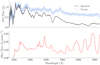 |
Fig. 10 SN ZTF20aamiflt spectrum – as extracted by HyperGal (black) and pysedm (blue) – and uniform sky spectrum (coefficient b0(λ), red). Flux unit fλ stands for femto-erg cm−2 s−1 Å−1. |
2.5.1 Integrated spectrum of the host galaxy
In summary, the host contribution can be isolated in the SEDM cube by subtracting the SN and the background components (see Fig. 11). To further compute an integrated host spectrum, a large elliptical aperture is defined around the host with the SEP package (Barbary 2016; Bertin & Arnouts 1996) from the PS 1 images. This aperture is then projected in the SEDM cube, using the respective World Coordinate Systems. We note that the ADR is neglected in the process, as it rarely induce a deviation of more than one or two spaxels in the FoV and has barely any impact on the host spectrum integrated over a large aperture.
The integrated host spectrum is shown in Fig. 11, with the expected position of some major emission lines at the input redshift (independently of the host spectrum). This procedure highlights the consistency between the input redshift used for the hyperspectral galaxy modeling and the extracted integrated spectrum. In the future, it could be considered as a way to consistently estimate the host’s redshift directly from such integrated spectrum during the scene modeling (see Sect. 4).
2.5.2 Point source radial profile
Similarly, the point source contribution can be isolated in the SEDM cube by subtracting both host and background models, as shown in Fig. 12 for the [6167, 6755] Å metaslice of the ZTF20aamifit cube. This closer look at the point source contribution allows us to check the accuracy of the PSF profile in each metaslice. The fact that the profile smoothly tends toward 0 means that the background was correctly modeled by HyperGal; also, the absence of outliers in the data points indicates that there is no evidence of residual host contamination in the profile, as noticed in the isolated SN image.
2.6 SN classification
As HyperGal is primarily designed for the transient spectral classification, an automated typing procedure is included in the pipeline, based on Supernova Identification (SNID Blondin & Tonry 2007). The process of typing is performed over the 4000 to 8000 Å spectral range, which includes the most discriminating spectral features for redshifts z ≲ 0.1. This domain also corresponds to the one where the SEDM CCD quantum efficiency is over 60%.
The quality of the snid classification is quantified by the rlap parameter, measuring the strength of the correlation between the input and template spectra. According to Blondin & Tonry (2007), an rlap ≥ 5 indicates a high confidence in the classification, without considering any prior on the redshift or the phase of the SN. Figure 13 presents the snid typing of ZTF20aamifit using its HyperGal-extracted spectrum. The best match has an rla p = 27, which leaves no doubt about its classification as an SN Ia. In comparison, the pysedm-extracted spectrum (see Fig. 10) is also typed as an SN Ia but with a significantly lower confidence (rlap = 9).
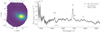 |
Fig. 11 ZTF20aamifit host galaxy, isolated from the SEDM data cube. Left panel: isolated host galaxy component in the SEDM cube, after subtraction of both the SN and background models. Right panel: host spectrum integrated over the selected spaxels; the main spectral features are marked for the input redshift z = 0.045. |
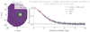 |
Fig. 12 SN ZTF20aamifit, isolated from the SEDM data cube. Left panel: isolated SN component in the SEDM [6167, 6755] Å metaslice, after subtraction of both the host and background models; the red cross indicates the fitted SN location, and contours show the elliptical isoradius at 3 and 5 spx for observations (black solid lines) and model (red dashed lines). Right panel: PSF profile for the same metaslice, as a function of the elliptical radius. The data points refer to the isolated SN on the left panel, the red curve corresponds to the PSF profile (without the background), the blue and the green curves to the Moffat and the Gaussian components, respectively. The Gaussian component is particularly weak because of the poor seeing conditions. |
3 HyperGal validation
The HyperGal pipeline was validated with a set of simulations, to quantify the accuracy of the extracted SN spectra as a function of various observational conditions and the ability to spectrally classify the transient. In this section, we first present the simulation process, before performing some statistical analysis on the spectral accuracy, followed by the typing efficiency. For comparison, the SNe are also extracted with a method similar to pysedm (Rigault et al. 2019), namely, a plain PSF extraction of a supposedly isolated source (not accounting for the background galaxy), but using the same PSF and diffuse background models as HyperGal for consistency.
3.1 Simulated sample
During a short shutdown of the main ZTF camera, SEDM was free to observe a few galaxies which hosted SNe at least 1 yr earlier. These observed host cubes are therefore naturally in the SEDM space for which HyperGal is designed; ten different hosts with various morphologies were acquired at different locations in the IFU and with an airmass ranging from 1.01 to 2.04. This allows us to cover a large variety of observation conditions, ranging from the ideal case to the poorest condition. An artificial point source, whose spectrum and type is known a priori, was then added to these cubes.
To mimic the SEDM spectra as closely as possible, we used the spectra of well-isolated transients observed with SEDM that had been successfully classified by snid with a very high rlap. For the SNe Ia (the most numerous to be observed), 70 spectra were selected with rlap > 25 for the best model and rlap > 15 for the first 30 models. Similarly, seven SNe II spectra with rlap > 12 were selected. For the more rarely observed SNe Ic and SNe Ib (~5% of observations), only one spectrum of each was chosen, but with a high classification confidence (rlap ~ 22 for the Ib and rlap ~ 13 for the Ic). To increase the S/N, each of these spectra was then slightly smoothed using a Savitzky-Golay filter (third-order polynomial over a window of five pixels) to keep the spectral structures intact.
While building the simulated sample, the different SN types were distributed to follow the observed fractions (Fremling et al. 2020), with 80% of SNe Ia, 15% of SNe II, 2.5% of SNe Ib, and 2.5% of SNe Ic. For further analysis, Ib and Ic will be studied jointly as SNe Ibc.
A marginalization on the phase of the SNe Ia was applied, based on the DR1 statistics from the ZTF SN Ia group (Dhawan et al. 2022). Knowing the phase of the 70 SN Ia input spectra used for the simulation, we composed the SN templates to follow the observed distribution of phases, modeled as a Gaussian distribution centered on −3 days with a standard deviation of 4 days.
Concerning the PSF, the profile is assumed to follow the model presented in Sect. 2.3.2. To faithfully represent the seeing diversity of the observations, the chromatic radial profile parameters were drawn from the joint distribution built from ~2000 standard stars, thus taking into account the latent correlations between parameters. Finally, two extra parameters − which we consider the most likely to impact the HyperGal robustness − were introduced in the simulations: the contrast, c, between the transient and the local background and the distance, d, between the target and the host.
The latter step aims to cover all observed cases, from the exact overlapping between the point source and the host (d ≈ 0) to the limit of an unstructured background (d ≫ host core size). The host center is identified by matching the WCS solution from the SEDM cube and the underlying photometric images from PS 1. The distance, d, is drawn from a uniform distribution between 0 and 5″. 6 ≡ 10 spx. As the SEDM mostly observes well-centered point sources, the simulated SN is placed within 12 spx from the center of the FoV, or at least toward the MLA center if the host is on the edge.
The contrast, c, is defined by c = S/(S + B) ϵ [0, 1], where S is the transient signal and B is the total (sky and host) background, both spectrally integrated over the equivalent r band of ZTF. For a random c drawn from a uniform distribution in [0, 1], the background signal B is first estimated at the simulated SN location, by successively integrating spatially the pure host cube weighted by the chromatic PSF profile, then spectrally over the ZTF r-band. Once B is known, the SN spectrum is scaled so that the r-band integral S = cB/(l – c). Finally, the simulated SN contribution to the cube variance is added to the one from the host galaxy, under the hypothesis of pure photon noise, using the flux solution of the host cube.
Ultimately, the 5000 simulated cubes were built, covering a large range of observation conditions, host galaxy morphologies and positions in the FoV, transient locations and spectral types, and S/N values. The HyperGal pipeline and the standard point source extraction were then used to estimate the resulting SN spectra.
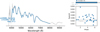 |
Fig. 13 snid typing of the ZTF20aamifit HyperGal spectrum. Left panel: input spectrum (in grey) and best model from snid (in blue). Right panel: distribution in the (redshift, phase) plane of the 30 best matches with an rlap > 5 (all being normal SNe la in this case). The input redshift of the galaxy (z = 0.045) is indicated with the horizontal grey line. The best model, with a very high rlap = 27, classifies ZTF20aamiflt as an SN la at redshift z = 0.046 and phase p = +5.6 days. |
3.2 Extraction accuracy
The SEDM is designed for and used in the spectral classification of transient. Thus, beyond pure absolute spectro-photometric flux accuracy, what is important is the capacity of HyperGal to extract the spectral features allowing for a proper classification, independently of the absolute flux level or even the large-scale continuum shape. Consequently, the HyperGal performances are evaluated on continuum-normalized transient spectra in the [4000, 8000] Å wavelength range, as in snid.
The continuum was fit as a fifth-order polynomial over the wavelength range slightly extended by 100 Å at each extreme, to avoid some unwanted boundary effects. The spectral comparison between simulation input and HyperGal/standard method output spectra was then systematically performed on continuum-normalized spectra and quantified using a wavelength-averaged relative rms similar to Eq. (5):
 (14)
(14)
where N refers to the number of monochromatic slices between [4000, 8000] Å, fλ denotes the data, and  the predicted value.
The distance, d, is found to have no influence on the spectral accuracy of HyperGal, with an absolute correlation coefficient lower than 0.2. On the other hand, Fig. 14 shows the correlation between spectral relative rms and contrast, c, for both extraction methods on continuum-normalized spectra. The results are marginalized over all SN types, as the extraction accuracy is supposedly independent of the spectral shape.
Both methods obtain an rms greater than 20% for c < 0.2, suggesting that spectral classification at such low contrast will be difficult. Yet, the standard method seems to be more accurate than HyperGal at extremely low contrast (c < 0.1); this actually appear to be an artifact of the continuum normalization. At very low contrast, neither method can reasonably disentangle the SN from the background; however, by effectively mixing the SN and host signal, the standard point source extracted spectrum has a higher S/N (albeit less accurate) and the continuum normalization is less prone to fail catastrophically, in contrast to the case of the spectrum consistent with 0 as extracted by HyperGal.
HyperGal starts to stand out for 0.2 < c < 0.3, with a median rms around 10%, and the rms decreases steadily below 10% at c > 0.3, 5% for c > 0.5, and 1% for c > 0.8. Compared to the standard extraction method, HyperGal shows a median improvement of ~50% for 0.2 < c < 0.6, and gradually returns to a median improvement of ~20% up to highest contrasts. Since the continuum normalization removes the effects of absolute scaling and color terms on the spectral rms, the improvement exclusively relates to the contamination of the SN spectrum by the host galaxy spectral features. This demonstrates the effectiveness of HyperGal in drastically reducing this host contamination.
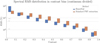 |
Fig. 14 Distribution, as a function of the contrast, of the spectral relative rms between simulation input spectra and extracted spectra, averaged over the [4000, 8000] Å domain. In the boxes, the 3 levels represent the 3 quartiles (25%, median, and 75%). Each bin includes the same number of simulations, as the contrast c is uniformly distributed in [0, 1]. |
3.3 Distribution of contrast in the observations
Before turning to the classification efficiency, the contrast distribution in the SEDM observations is estimated, as a reference for a comparison with our results. Rather than using HyperGal on observations made with the SEDM (as was actually done for the ZTF Cosmology SN la Data Release 2 by Rigault et al., in prep.), which would be akin to evaluating the pipeline with itself, instead the contrast c = S/(S + B) was estimated from photometric images of the same DR2 sample, made up of about 3000 SNe la.
For each SN, its signal S in the PS 1 r-band at the date of the SEDM observation was estimated from the SALT2 fit (Guy et al. 2005, 2007; Betoule et al. 2014) of its light curve. We chose the PS 1 r band which, in practice, is very similar to the ZTF one and because only these images from the survey were available at the time of the study. On the other hand, the host contribution to the background, Bgal was estimated from the integrated flux within a radius of 2″ around the SN. As the PS 1 images are already sky-subtracted, an additional sky background, Bsky, had to be added for a fair comparison with simulations. Two different values were used: a fiducial value of msky = 20 mag, approximately corresponding to the magnitude depth of the SEDM, and a more conservative value, msky = 21 mag. Given the sky background is largely negligible in front of a galactic one, its exact value essentially alters the high contrast values: for a SN isolated from its host galaxy, the contrast would systematically increases as the sky background tends toward 0.
Figure 15 displays the cumulative distribution of the contrast for the DR2. The median contrast of this distribution is c = 0.58 for msky = 20 mag and c = 0.63 for msky = 21 mag. For both sky levels, less than 1% of observations have a contrast c < 0.1, and only 7% with c < 0.2. At the high-contrast end, 2–5% of the observations have a c > 0.9 depending on the adopted sky magnitude. Almost 95% of observations have a contrast 0.1 < c < 0.9, and a slightly less than 90% with 0.2 < c < 0.9.
According to the results of Sect. 3.2, we can therefore assess the spectral accuracy of HyperGal on the DR2 sample (using the spectral relative rms (Eq. (14)) as an indicator) to be on the order of 10%, 5%, and 2% for 80%, 60%, and 20% of the observations, respectively. In comparison, the standard extraction method reaches these levels for 60%, 45%, and 15% of the observations.
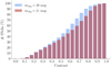 |
Fig. 15 Cumulative contrast distribution estimated from ~3000 SN la observed with the SEDM. Since only Bgal is estimated from PS 1 images, an additional Bsky is estimated using two different sky levels, msky = 20 (blue) for a realistic value and msky = 21 (red) for a conservative value. |
3.4 Typing efficiency
As mentioned earlier, the most important validation result in the context of the SEDM is the efficiency of HyperGal to spectrally classify the target SN. The test on the simulated cubes was performed using the same classifier as in ZTF, namely, SNID; the confidence criteria given for the classification are however slightly stricter, as we regularly identified false positives (i.e., SN erroneously classified as Ia) in the current pysedm pipeline. The minimum rlap is set to  (rather than 5) for the best-fit model; furthermore, at least 50% of the top-10 models have to be of the same type as the best one to confirm a classification. If one of these criteria is not met, the spectrum is classified as “uncertain”.
Figure 16 shows the typing efficiency from HyperGal and the improvement with respect to the standard extraction method without host modeling. Contrary to the previous rms analysis, results are presented for each SN type, since the spectral signatures are different in all SN types.
As anticipated in Sect. 3.2, both methods are definitely not reliable for contrasts below 0.1. SNe Ia are more easily classified, due to the quantity and strength of features in their spectra: the typing success is 71% for SNe Ia for 0.1 < c < 0.2 (~7% of real observations); types Ibc and II, on the other hand, are correctly classified with a success rate of 23% and 35%, respectively.
For 0.2 < c < 0.3, the typing success reaches more than 96% for SNe Ia, 77% for Ibc and 51% for SNe II. More than 99% of SNe Ia are correctly classified with c > 0.3, and more than 95% of all SNe for c > 0.4. With ~84% of observations having a contrast c > 0.3, ~9% with 0.2 < c < 0.3, and ~7% with 0.1 < c < 0.2, we can conclude that HyperGal is able to successfully classify nearly 95% of all SNe Ia observed by SEDM. For a contrast of c > 0.2 (which represents more than 90% of the real observations), nearly 99% of SNe Ia are properly classified. The improvement brought by HyperGal over the standard extraction method is obvious, with a sweet spot in 0.1 < c < 0.6: this will results in more than 30% of additional SNe correctly classified.
The main spectral feature of SNe II being the Ha emission line, usually highly contaminated by the host galaxy, HyperGal allows a significant improvement for this particular type, from 15% to 37% of additional correctly classified SNe II in the 0.1 < c < 0.6 range; for SNe Ibc, the difference only appears from c > 0.2, with similar gains between 13% and 31%. SNe Ia exhibits a lot of strong and easily identified spectral features, the boost from the standard method is slightly less obvious, but remains, in fact, highly significant, from 30% of additional correctly classified SNe Ia for 0.1 < c < 0.2 to 5% when 0.5 < c < 0.6. For c > 0.6, when the SN ostensibly stands out of the galaxy, the difference between the two methods becomes marginal whatever the SN type.
Taking into account the contrast distribution of the observations, HyperGal should significantly improve the classification of SNe Ia in nearly 50% of the observations (the other half being also properly classified by the standard extraction method). As 50% of the observations have 0.1 < c < 0.6, HyperGal will allow the correct classification of almost 20% more SNe Ia in this interval, corresponding to 10% of all SNe Ia classifiable with the SEDM. Assuming a similar contrast distribution for all SN types, HyperGal is expected to classify 14% additional SNe II and 11% SNe Ibc.
To probe the critical contamination of the SN la sample by core-collapse SNe, the false-positive rate (FPR) for SN la is examined. Figure 17 shows that HyperGal has a significantly lower FPR than for the standard method. Excluding the unrealistically low contrast cases (c < 0.1), HyperGal shows a progressive decrease in FPR from 8% to 1% for contrast rising from 0.1−0.6 (FPR is null beyond that); in comparison, the standard method oscillates between 6 and 9% in same contrast range. As a conclusion, the HyperGal FPR is on average less than 5% for contrasts between 0.1 and 0.6 (~50% of the observations), and less than 2% for c> 0.1 (more than 99% of all observations); this is half the result of the standard extraction method.
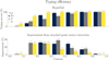 |
Fig. 16 Typing efficiency on the validation simulations. Top panel: rate of successful classification with HyperGal for each type of SN at different contrast levels. Results for c > 0.6 are aggregated as the results vary very little. Bottom panel: improvement in typing compared to the standard extraction method. |
 |
Fig. 17 False-positive rate in SN la classification for both extraction methods as a function of contrast. |
4 Discussion
Here, we discuss some limitations of the current HyperGal implementation and possible future developments. Regarding the validation methodology, we acknowledge some simplifications with respect to actual observations. For instance, the true distance distribution between the SN and its host was not explicitly modeled, for instance, this parameter was marginalized uniformly between 0 and 576. As a full-scene modeler which properly handles this parameter and therefore shows little sensitivity to it (Sect. 3.2), this approximation does not impact the HyperGal results; this is not true for the single point-source method which critically depends on the transient-host distance. Overall, we think the validation approximations actually tend to minimize the improvement of HyperGal with respect to the standard method.
Undoubtedly, the most limiting constraint from HyperGal is the need for an external redshift measurement of the host galaxy, a priori needed by the SED fitter used as a physically motivated host galaxy spectral interpolator and of critical importance for the treatment of emission lines. In practice, this is not so much of an issue: in the current ZTF sample, about 50% of SN hosts already have a spectral redshift, mostly from SDSS surveys (Fremling et al. 2020), with a precision of σz ~ 10−5 for z < 0.1 (Bolton et al. 2012); the remaining 50% of SNe have a red-shift deduced from a preliminary extraction of the SN spectrum, either from low-resolution spectral features in the SN spectrum (~40%) or emission lines of the host galaxy having contaminated the SN spectrum (~10%). In both cases, the redshift is estimated by SNID with a precision of σz ~ 5 × 10⁻³ (Fremling et al. 2020). Furthermore, 95% of ZTF SN hosts are brighter than 20 mag, paving the way for other surveys such as the Dark Energy Spectroscopic Instrument (DESI) Bright Galaxy Survey (DESI Collaboration 2016) to systematically provide a large fraction of spectral redshifts in the future.
A slightly incorrect input redshift (encoded as a wavelength offset of the emission line position in the hyperspectral galaxy model), as well as an approximate SED fit of the emission line fluxes (marginally constrained by broadband photometric observations) is corrected to first order by the monochromatic galaxy amplitudes G(λ) during the ultimate 3D fit. Primarily introduced to recover flux calibration mismatch between PS1 and SEDM, this normalization parameter actually interferes in a non-trivial way with the position and intensity of emission lines in the brightest parts of the scene to minimize residuals between fixed (at this stage of the procedure) hyperspectral model and SEDM observations. This particular effect, which depends on the relative distribution of stellar and gaseous components in the host, has not been studied extensively for HyperGal, but we note it is efficient to disentangle host spectral features from SN spectrum even with sub-optimal input redshift or emission line fluxes. However, it effectively precludes the use of the residual host component for any a posteriori measurements, for instance, redshift or local measurement of Ha flux, yet crucial for local environment studies mentioned earlier (e.g., Rigault et al. 2020).
It is possible to think of including a consistent redshift estimate directly in the HyperGal procedure, at the level of the hyperspectral model (to minimize artificial fluctuations of G(λ)), but also at the level of the SN spectral typing (to reach a red-shift consensus between the host and the SN). This would imply to include the intensive SED fit or the SN typing procedure in the minimization loop, which is computationally costly in either case. Another major HyperGal development would be to use the SEDM cube, a rich and faithful observation of the host galaxy at the position of the transient, as additional hyperspectral constraints in the SED fitting process. Both developments would push the concept of an SED fitter merely used as a spectral interpolator to its limit. It would then probably be preferable to switch to other more efficient methods, such as physics-enabled deep learning (Boone 2021).
5 Conclusion
This paper presents HyperGal, a fully automated scene modeler for the transient typing with the SEDM (Blagorodnova et al. 2018). The core of this pipeline is based on the use of archival photometric observations of the host galaxy, taken before the SN explosion. Knowing the physical processes in place within galaxies, as encoded in the SED fitter cigale, the spectral properties of the host are modeled, adjusted, and scaled appropriately to create a hyperspectral model of the host galaxy. This 3D intrinsic model is then convolved with the spectro-spatial instrumental responses of the SEDM, and projected in the space of the observations. A full scene model, including the structured host galaxy, the point source transient and a smooth background, is finally produced to match the SEDM observations, allowing for the extraction of the SN spectrum from a highly contaminated environment.
The pipeline is validated on a large set of realistic simulated SEDM observations, covering a wide variety of observation conditions (airmass, seeing, and PSF parameters), scene details (host morphology, distance to the host, host/SN contrast), and transient types. The contrast distribution is estimated from about 3000 observed SNe la of the upcoming ZTF Cosmology SN la DR2 paper (Rigault et al., in prep.). The transient spectra in the 5000 simulations are then extracted with HyperGal and compared to the historical point-source method, which ignores the structured host component.
The most important results concern HyperGal efficiency in spectroscopically typing SNe, a key objective of the SEDM instrument. The full scene modeler shows an ability to correctly classify ~95% of the observed SNe la under a realistic contrast distribution. For a contrast c > 0.2 (more than 90% of the observations), nearly 99% of the SNe la are correctly classified. Compared to the standard extraction method, HyperGal correctly classifies nearly 20% more SNe la between 0.1 < c < 0.6, representing ~50% of the observation conditions.
The false positive rate for HyperGal is less than 5% for contrasts between 0.1 and 0.6, and less than 2% for c > 0.1 (>99% of the observations); this is half as much as the standard extraction method. HyperGal has demonstrated its ability to extract and classify the spectrum of an SN even in the presence of strong contamination from its host galaxy. The improvement compared to the standard method is significant: this will noticeably improve the statistics of the SNe Ia sample for the ZTF survey, while reducing a potential environmental bias, ultimately impacting the precision of cosmological analyses.
Acknowledgements
This project has received funding from the Project IDEX-LYON at the University of Lyon, under the Investments for the Future Program (ANR-16-IDEX-0005), and from the European Research Council (ERC) under the European Union’s Horizon 2020 research and innovation programme (grant agreement no. 759194 – USNAC). The SED Machine is based upon work supported by the National Science Foundation under Grant No. 1106171. Based on observations obtained with the Samuel Oschin Telescope 48-in. and the 60-in. Telescope at the Palomar Observatory as part of the Zwicky Transient Facility project. ZTF is supported by the National Science Foundation under Grant No. AST-1440341 and a collaboration including Caltech, IPAC, the Weiz-mann Institute for Science, the Oskar Klein Center at Stockholm University, the University of Maryland, the University of Washington, Deutsches Elektronen-Synchrotron and Humboldt University, Los Alamos National Laboratories, the TANGO Consortium of Taiwan, the University of Wisconsin at Milwaukee, and Lawrence Berkeley National Laboratories. Operations are conducted by COO, IPAC, and UW. This research made use of python (Van Rossum & Drake 2009), astropy (Astropy Collaboration 2013, 2018), matplotlib (Hunter 2007), numpy (van der Walt et al. 2011; Harris et al. 2020), scipy (Jones et al. 2001; Virtanen et al. 2020). We thank their developers for maintaining them and making them freely available.
References
- Astropy Collaboration (Robitaille, T. P., et al.) 2013, A&A, 558, A33 [NASA ADS] [CrossRef] [EDP Sciences] [Google Scholar]
- Astropy Collaboration (Price-Whelan, A. M., et al.) 2018, AJ, 156, 123 [Google Scholar]
- Barbary, K. 2016, J. Open Source Softw., 1, 58 [Google Scholar]
- Battisti, A. J., Calzetti, D., & Chary, R. R. 2016, ApJ, 818, 13 [NASA ADS] [CrossRef] [Google Scholar]
- Bellm, E. C., Kulkarni, S. R., Graham, M. J., et al. 2019, PASP, 131, 018002 [Google Scholar]
- Bertin, E., & Arnouts, S. 1996, A&AS, 117, 393 [NASA ADS] [CrossRef] [EDP Sciences] [Google Scholar]
- Betoule, M., Kessler, R., Guy, J., et al. 2014, A&A, 568, A22 [NASA ADS] [CrossRef] [EDP Sciences] [Google Scholar]
- Blagorodnova, N., Neill, J. D., Walters, R., et al. 2018, PASP, 130, 035003 [Google Scholar]
- Blondin, S., & Tonry, J. L. 2007, ApJ, 666, 1024 [NASA ADS] [CrossRef] [Google Scholar]
- Bolton, A. S., Schlegel, D. J., Aubourg, É., et al. 2012, AJ, 144, 144 [NASA ADS] [CrossRef] [Google Scholar]
- Boone, K. 2021, AJ, 162, 275 [NASA ADS] [CrossRef] [Google Scholar]
- Boquien, M., Burgarella, D., Roehlly, Y., et al. 2019, A&A, 622, A103 [NASA ADS] [CrossRef] [EDP Sciences] [Google Scholar]
- Briday, M., Rigault, M., Graziani, R., et al. 2022, A&A, 657, A22 [NASA ADS] [CrossRef] [EDP Sciences] [Google Scholar]
- Bruzual, G., & Charlot, S. 2003, MNRAS, 344, 1000 [NASA ADS] [CrossRef] [Google Scholar]
- Buat, V., Boquien, M., Malek, K., et al. 2018, A&A, 619, A135 [NASA ADS] [CrossRef] [EDP Sciences] [Google Scholar]
- Burgarella, D., Buat, V., & Iglesias-Páramo, J. 2005, MNRAS, 360, 1413 [NASA ADS] [CrossRef] [Google Scholar]
- Buton, C., Copin, Y., Aldering, G., et al. 2013, A&A, 549, A8 [NASA ADS] [CrossRef] [EDP Sciences] [Google Scholar]
- Chabrier, G. 2003, PASP, 115, 763 [Google Scholar]
- Chambers, K. C., Magnier, E. A., Metcalfe, N., et al. 2016, arXiv e-prints [arXiv: 1612.05560] [Google Scholar]
- Charlot, S., & Fall, S. M. 2000, ApJ, 539, 718 [Google Scholar]
- Chevallard, J., Curtis-Lake, E., Charlot, S., et al. 2019, MNRAS, 483, 2621 [NASA ADS] [CrossRef] [Google Scholar]
- Childress, M., Aldering, G., Antilogus, P., et al. 2013, ApJ, 770, 107 [NASA ADS] [CrossRef] [Google Scholar]
- da Cunha, E., Charlot, S., & Elbaz, D. 2008, MNRAS, 388, 1595 [Google Scholar]
- Dale, D. A., Helou, G., Magdis, G. E., et al. 2014, ApJ, 784, 83 [Google Scholar]
- Dask Development Team. 2016, Dask: Library for dynamic task scheduling Dembinski, H., Ongmongkolkul, P., Deil, C., et al. 2020, https://doi.org/10.5281/zenodo.3949207 [Google Scholar]
- DESI Collaboration (Aghamousa, A., et al.) 2016, arXiv e-prints [arXiv: 1611.00036] [Google Scholar]
- Dhawan, S., Goobar, A., Smith, M., et al. 2022, MNRAS, 510, 2228 [NASA ADS] [CrossRef] [Google Scholar]
- Drake, A. J., Djorgovski, S. G., Mahabal, A., et al. 2009, ApJ, 696, 870 [Google Scholar]
- Fremling, C., Miller, A. A., Sharma, Y., et al. 2020, ApJ, 895, 32 [NASA ADS] [CrossRef] [Google Scholar]
- Gillies, S. et al. 2007, Shapely: manipulation and analysis of geometric objects [Google Scholar]
- Graham, M. J., Kulkarni, S. R., Bellm, E. C., et al. 2019, PASP, 131, 078001 [Google Scholar]
- Guy, J., Astier, P., Baumont, S., et al. 2007, A&A, 466, 11 [NASA ADS] [CrossRef] [EDP Sciences] [Google Scholar]
- Guy, J., Astier, P., Nobili, S., Regnault, N., & Pain, R. 2005, A&A, 443, 781 [NASA ADS] [CrossRef] [EDP Sciences] [Google Scholar]
- Harris, C. R., Millman, K. J., van der Walt, S. J., et al. 2020, Nature, 585, 357 [NASA ADS] [CrossRef] [Google Scholar]
- Hunter, J. D. 2007, Comput. Sci. Eng., 9, 90 [NASA ADS] [CrossRef] [Google Scholar]
- Inoue, A. K. 2011, MNRAS, 415, 2920 [NASA ADS] [CrossRef] [Google Scholar]
- James, F., & Roos, M. 1975, Comput. Phys. Commun., 10, 343 [Google Scholar]
- Jones, E., Oliphant, T., & Peterson, P. 2001, SciPy: Open Source Scientific Tools for Python [Google Scholar]
- Jones, D. O., Scolnic, D. M., Riess, A. G., et al. 2017, ApJ, 843, 6 [NASA ADS] [CrossRef] [Google Scholar]
- Jordahl, K. 2014, GeoPandas: Python tools for geographic data [Google Scholar]
- Kaiser, N., Aussel, H., Burke, B. E., et al. 2002, SPIE Conf. Ser., 4836, 154 [Google Scholar]
- Kelly, P. L., Hicken, M., Burke, D. L., Mandel, K. S., & Kirshner, R. P. 2010, ApJ, 715, 743 [Google Scholar]
- Kim, Y. L., Rigault, M., Neill, J. D., et al. 2022, PASP, 134, 024505 [NASA ADS] [CrossRef] [Google Scholar]
- Law, N. M., Kulkarni, S. R., Dekany, R. G., et al. 2009, PASP, 121, 1395 [NASA ADS] [CrossRef] [Google Scholar]
- Malek, K., Buat, V., Roehlly, Y., et al. 2018, A&A, 620, A50 [NASA ADS] [CrossRef] [EDP Sciences] [Google Scholar]
- Noll, S., Burgarella, D., Giovannoli, E., et al. 2009, A&A, 507, 1793 [NASA ADS] [CrossRef] [EDP Sciences] [Google Scholar]
- Pruzhinskaya, M. V., Novinskaya, A. K., Pauna, N., & Rosnet, P. 2020, MNRAS, 499, 5121 [NASA ADS] [CrossRef] [Google Scholar]
- Rigault, M., Copin, Y., Aldering, G., et al. 2013, A&A, 560, A66 [NASA ADS] [CrossRef] [EDP Sciences] [Google Scholar]
- Rigault, M., Aldering, G., Kowalski, M., et al. 2015, ApJ, 802, 20 [Google Scholar]
- Rigault, M., Neill, J. D., Blagorodnova, N., et al. 2019, A&A, 627, A115 [NASA ADS] [CrossRef] [EDP Sciences] [Google Scholar]
- Rigault, M., Brinnel, V., Aldering, G., et al. 2020, A&A, 644, A176 [NASA ADS] [CrossRef] [EDP Sciences] [Google Scholar]
- Rubin, D., Aldering, G., Antilogus, P., et al. 2022, ApJS, 263, 1 [NASA ADS] [CrossRef] [Google Scholar]
- Shappee, B. J., Prieto, J. L., Grupe, D., et al. 2014, ApJ, 788, 48 [Google Scholar]
- Stone, J., & Zimmerman, J. 2001, Index of Refraction of Air [Google Scholar]
- Sullivan, M., Conley, A., Howell, D. A., et al. 2010, MNRAS, 406, 782 [NASA ADS] [Google Scholar]
- Tonry, J. L., Stubbs, C. W., Lykke, K. R., et al. 2012, ApJ, 750, 99 [Google Scholar]
- Tonry, J. L., Denneau, L., Heinze, A. N., et al. 2018, PASP, 130, 064505 [Google Scholar]
- van der Walt, S., Colbert, S. C., & Varoquaux, G. 2011, Comput. Sci. Eng., 13, 22 [Google Scholar]
- Van Rossum, G., & Drake, F. L. 2009, Python 3 Reference Manual (CreateSpace) [Google Scholar]
- Virtanen, P., Gommers, R., Oliphant, T. E., et al. 2020, Nat. Methods, 17, 261 [Google Scholar]
- Waters, C. Z., Magnier, E. A., Price, P. A., et al. 2020, ApJS, 251, 4 [NASA ADS] [CrossRef] [Google Scholar]
The code is available online at https://github.com/JeremyLezmy/HyperGal
Version 2020, https://cigale.lam.fr
All Tables
All Figures
|
Fig. 1 Main processing steps of the HyperGal pipeline and sections where they are detailed. |
| In the text | |
|
Fig. 2 SEDM cube from the observation of ZTF20aamifit. Left panel shows the spectra, whose color corresponds to the selected spaxels in the right panel (white image of the spectrally integrated cube). Red cross shows the SN position. |
| In the text | |
|
Fig. 3 RGB image of the host galaxy of SN ZTF20aamifit, constructed from the PS1 grz cutouts. The red cross shows the position of the SN detected by ZTF. The x- and y-axes are in native PS1 pixels, 0725 aside. White dashed box is used as the boundaries in Figs. 4 and 6. |
| In the text | |
|
Fig. 4 Map of the pull for the grizy broadband images from cigale outputs, and spectral relative rms over the five reference host images, shown from left to right and top to bottom. Only pixels with S/N > 3 for all grizy bands are considered (see Sect. 2.2). |
| In the text | |
|
Fig. 5 LSF standard deviation, σLSF, as a function of wavelength, from the wavelength calibration of 65 nights between 2018 and 2022. Each violin corresponds to an emission line in the arc-lamp spectra (color legend). |
| In the text | |
|
Fig. 6 Hyperspectral galaxy model of ZTF20aamifit host galaxy, after projection in the SEDM observation space (including LSF). Green circles correspond to the spatially integrated flux from PS1 cutouts, while black diamonds refer to the same quantities as fit by cigale. The five shaded curves show the transmission of the grizy PS1 filters. Red and blue spectra on the left correspond to the spectra integrated in selected regions of same color in the model cube on the right. The black spectrum is the spectrum integrated over the full FoV. |
| In the text | |
|
Fig. 7 Fit result for the [6167, 6755] Å metaslice of ZTF20aamifit cube. From left to right: metaslice from the original (transient-free) hyperspectral model with MLA footprint overplotted, projected fitted scene (host + background + SN), SEDM observations, and relative model residuals. |
| In the text | |
|
Fig. 8 SN positions as a function of wavelength, and the effective ADR fit. Top panel: relative offsets with respect to reference position at reference wavelength along each axis; filled points correspond to the observed offsets, and open circles to the predictions of the ADR model. Bottom panel: relative offsets in the (x, y) plane. Color codes refer to the central wavelength of the metaslices. |
| In the text | |
|
Fig. 9 Full scene model for ZTF20aamifit. Top panel: integrated SEDM and HyperGal-modeled cubes; the red cross indicates the adjusted point source position at 6000 A. Bottom panel: spectral pull and spectral relative rms. No galaxy- or SN-related structured residual is visible in the pull map and the spectral rms indicates an accuracy of ~4% at the host and SN locations. |
| In the text | |
|
Fig. 10 SN ZTF20aamiflt spectrum – as extracted by HyperGal (black) and pysedm (blue) – and uniform sky spectrum (coefficient b0(λ), red). Flux unit fλ stands for femto-erg cm−2 s−1 Å−1. |
| In the text | |
|
Fig. 11 ZTF20aamifit host galaxy, isolated from the SEDM data cube. Left panel: isolated host galaxy component in the SEDM cube, after subtraction of both the SN and background models. Right panel: host spectrum integrated over the selected spaxels; the main spectral features are marked for the input redshift z = 0.045. |
| In the text | |
|
Fig. 12 SN ZTF20aamifit, isolated from the SEDM data cube. Left panel: isolated SN component in the SEDM [6167, 6755] Å metaslice, after subtraction of both the host and background models; the red cross indicates the fitted SN location, and contours show the elliptical isoradius at 3 and 5 spx for observations (black solid lines) and model (red dashed lines). Right panel: PSF profile for the same metaslice, as a function of the elliptical radius. The data points refer to the isolated SN on the left panel, the red curve corresponds to the PSF profile (without the background), the blue and the green curves to the Moffat and the Gaussian components, respectively. The Gaussian component is particularly weak because of the poor seeing conditions. |
| In the text | |
|
Fig. 13 snid typing of the ZTF20aamifit HyperGal spectrum. Left panel: input spectrum (in grey) and best model from snid (in blue). Right panel: distribution in the (redshift, phase) plane of the 30 best matches with an rlap > 5 (all being normal SNe la in this case). The input redshift of the galaxy (z = 0.045) is indicated with the horizontal grey line. The best model, with a very high rlap = 27, classifies ZTF20aamiflt as an SN la at redshift z = 0.046 and phase p = +5.6 days. |
| In the text | |
|
Fig. 14 Distribution, as a function of the contrast, of the spectral relative rms between simulation input spectra and extracted spectra, averaged over the [4000, 8000] Å domain. In the boxes, the 3 levels represent the 3 quartiles (25%, median, and 75%). Each bin includes the same number of simulations, as the contrast c is uniformly distributed in [0, 1]. |
| In the text | |
|
Fig. 15 Cumulative contrast distribution estimated from ~3000 SN la observed with the SEDM. Since only Bgal is estimated from PS 1 images, an additional Bsky is estimated using two different sky levels, msky = 20 (blue) for a realistic value and msky = 21 (red) for a conservative value. |
| In the text | |
|
Fig. 16 Typing efficiency on the validation simulations. Top panel: rate of successful classification with HyperGal for each type of SN at different contrast levels. Results for c > 0.6 are aggregated as the results vary very little. Bottom panel: improvement in typing compared to the standard extraction method. |
| In the text | |
|
Fig. 17 False-positive rate in SN la classification for both extraction methods as a function of contrast. |
| In the text | |
Current usage metrics show cumulative count of Article Views (full-text article views including HTML views, PDF and ePub downloads, according to the available data) and Abstracts Views on Vision4Press platform.
Data correspond to usage on the plateform after 2015. The current usage metrics is available 48-96 hours after online publication and is updated daily on week days.
Initial download of the metrics may take a while.