| Issue |
A&A
Volume 668, December 2022
|
|
|---|---|---|
| Article Number | A150 | |
| Number of page(s) | 23 | |
| Section | Astronomical instrumentation | |
| DOI | https://doi.org/10.1051/0004-6361/202243465 | |
| Published online | 16 December 2022 | |
Characterization of the Microlensed Hyperspectral Imager prototype
1
Max Planck Institute for Solar System Research,
Justus-von-Liebig-Weg 3,
37077
Göttingen, Germany
e-mail: This email address is being protected from spambots. You need JavaScript enabled to view it.
2
European Space Agency via Aurora Technology B.V.,
Zwarteweg 39,
2201 AA
Noordwijk, The Netherlands
Received:
3
March
2022
Accepted:
15
August
2022
Abstract
Context. The Microlensed Hyperspectral Imager (MiHI) prototype is an integral field spectrograph based on a double-sided microlens array (MLA), installed as an extension to the TRIPPEL spectrograph at the Swedish Solar Telescope (SST).
Aims. Due to the mixing of spatial and spectral information in the focal plane, the data are mapped in an interleaved way onto the image sensor. Mapping the information back into its original spatial and spectral dimensions renders the data reduction more complex than usual, and requires the development of a new reduction procedure.
Methods. The mapping of the data onto the detector is calculated using a simplified model of the image formation process. Since the moiré fringes that are formed due to the interference of the pixel grid and the MLA grid are a natural consequence of this formation process, the extraction of the data using such a model should eliminate them from the data cubes, thereby eliminating the principal source of instrumentally induced artifacts. In addition, any change in the model caused by small movements of the raw image on the detector can be fitted and included in the model.
Results. An effective model of the instrument was fitted using a combination of the numerical results obtained for the propagation of light through an ideal dual microlens system, complemented with an ad hoc fit of the optical performance of the instrument and the individual elements in the MLA. The model includes individual fits for the position, focus, focus gradient, coma, and a few high-order symmetric modes, which are required to account for the spectral crosstalk within each image row. The model is able to accurately reproduce the raw flat-field data from a hyperspectral cube that is virtually free of moiré fringes, and it represents a critical first step in a new hyperspectral data reduction procedure.
Key words: techniques: imaging spectroscopy / techniques: image processing / methods: numerical / methods: data analysis
© M. van Noort and A. Chanumolu 2022
 Open Access article, published by EDP Sciences, under the terms of the Creative Commons Attribution License (https://creativecommons.org/licenses/by/4.0), which permits unrestricted use, distribution, and reproduction in any medium, provided the original work is properly cited.
This article is published in open access under the Subscribe-to-Open model.
Open Access funding provided by Max Planck Society.
1 Introduction
An essential step in the design and development of any instrument is the determination of the response of the instrument to a known input, the calibration (see e.g. Webster 1999; Northrop 2014.). This activity can vary widely, from the determination of the response of the instrument to known signals, to the development of an elaborate model, constrained by calibration measurements.
Astronomical instruments used for solar observations can be roughly divided in two main categories, spectrographic instruments that use a spatial filter (usually a slit mask) and a dispersive element to generate a spatio-spectral image, and imaging instruments that generate an image at a specific wavelength using a spectral filter to select a given wavelength band. Since it is possible to build spectrographic instruments that are almost perfectly able to separate the spatial and spectral dimensions, their calibration is generally relatively straightforward (e.g., Pereira et al. 2009; Chae et al. 2013). It typically consists of assuming that the spectrum seen by all spatial pixels is the same; fitting the wavelength scale, position, and spectral point-spread function (PSF) for each spatial position along the slit mask; and dividing out the spectrum to obtain a map of the instrumental transmission. The inverse application of this information is usually sufficient to produce calibrated data of satisfactory quality.
The data produced by narrow-band imagers is usually more of a mixture of spatial and spectral information, and their reduction pipelines, therefore, must first be able to separate this information before an accurate calibration can be carried out. Especially tunable filter imagers usually have long and complicated reduction pipelines, since any deviation from perfection inevitably leads to the mixing of spatial and spectral information. This can make it difficult to separate the spectral response from a spatial variation of the instrumental transmission properties, which in addition can differ from tuning position to tuning position. Such pipelines often still can make use of the basic principle underlying the calibration of most imaging and spectral instruments, that of assumed spatial uniformity of the spectrum. However, they do not use the data to directly measure the spatio-spectrally averaged spectrum, but rather to constrain a model of the true spectrum seen by all spatial pixels, which is then sampled by an instrument with an imperfect response (e.g., van Noort & Rouppe van der Voort 2008; Schnerr et al. 2011; de la Cruz Rodríguez et al. 2015).
The Microlensed Hyperspectral Imager (MiHI) prototype is an integral field spectrograph (IFS), described in van Noort et al. (2022, hereafter Paper I), which projects light from two spatial and one spectral dimension onto a 2D image sensor, so that all information in a specific spatio-spectral cube is recorded simultaneously. In order to obtain an accurately calibrated 3D hyperspectral cube from such images, the encoded information must first be extracted, which presents a number of challenges that are not encountered in other types of instruments. At present, IFSs are not widely used for solar observations, and calibration strategies for them using solar data have not been described in the literature. However, IFSs are not new to the field of astronomy in general, and a number of them have been constructed and operated for decades on major telescopes.
Two of the most widely used types of IFS that are currently in use are those based on arrays of lenslets or microlenses (e.g. TIGER, Bacon et al. 1995; OSIRIS, Bacon et al. 2000; Larkin et al. 2006; SAURON, Bacon et al. 2001) and those based on image slicers (e.g. SINFONI, Tecza et al. 2000; MUSE, Henault et al. 2003). These instruments were designed to study the dynamics of spatially resolved extended objects, such as galaxies, stellar clusters, and molecular clouds, and typically have a limited spectral resolution of 4000 or less, in favor of the largest field of view (FOV) that can be fitted onto the available detector(s).
The second generation of such instruments (e.g. GPI, Macintosh et al. 2006; CHARIS, Groff et al. 2014; SPHERE, Beuzit et al. 2019) were developed primarily for the observation of exoplanets, which requires them to operate at the highest spatial resolution that can be obtained by the telescope. To provide the required optical performance while operating at the telescope diffraction limit, some of them employ a double-sided microlens solution (BIGRE, Antichi et al. 2009), similar to the MiHI prototype.
To convert IFS images into 3D hyperspectral cubes, the most straightforward strategy is to map each image pixel on the detector to an element from the hyperspectral data cube, and simply extract it from the raw data cube. While this may result in a useable data cube for critically sampled or oversampled raw images, it is unlikely to collect all the signal that is present in the data, and cannot discriminate between light from the target spectrum and that from other sources, such as scattered light, or instrumentally induced cross-contamination from other spectra. A popular way to address these problems, used in a number of extraction algorithms for existing IFS data reduction pipelines (e.g., Bacon et al. 2001; Pavlov et al. 2008), is to characterize the instrumental cross-dispersion properties (i.e. the line-spread function) and using this information as a constraint to extract the spectral information in an optimal way (Horne 1986; Robertson 1986). To extract the spectra with the highest level of accuracy, we must determine not just the location of each spatio-spectral element on the detector or the crosstalk of one spectrum to its nearest neighbors, but describe the formation of the image on the detector in considerable detail and in two dimensions. Such an approach is outlined in Berdeu et al. (2020) and stands at the basis of their PIC data reduction algorithm for the reduction of IFS data.
The data of the MiHI prototype somewhat differ from that of other IFS instruments, in that it samples the image plane at the highest spatial resolution, on a regular spatial grid, and at a spectral resolution that is in excess of 300 000, considerably higher than that of any of the instruments mentioned above. In addition, the data are often degraded significantly by atmospheric seeing, so that the contrast of a solar observation rarely exceeds 10% at continuum wavelengths in the visible part of the spectrum. For the data to be suitable for restoration to their undegraded state by numerical means (by using an image restoration technique such as speckle (Lohmann et al. 1983; von der Luehe 1993) or MFBD (Löfdahl & Scharmer 1994; van Noort et al. 2005)), a standard part of the reduction pipeline of most instruments for solar observations, residual errors in the extracted data must be brought well below the noise level of the restored data. In this paper, we seek to extract hyperspectral cubes from the raw data with an accuracy that is sufficient for the subsequent application of image restoration, using the PIC algorithm. To this end, we set out to develop a model of the MiHI prototype, a key step in the construction of a highly accurate data extraction and reduction pipeline. The construction of that pipeline and the subsequent restoration of the data to a high-resolution data cube will be the subject of van Noort & Doerr (2022, hereafter Paper III).
2 Instrument characterization
The design of the MiHI prototype, described in Paper I, is based on a double-sided microlens array (MLA) that is used to optically sample the image plane, and demagnify each sample, resulting in an array of bright, point-like sources, in an otherwise dark plane. When the image is then passed through a spectrograph, each bright source is dispersed in the dark space, generating a spectrum for each source, without overlapping significantly with the spectra of any of the other sources over a selected spectral band. The MLA is designed to generate critically sampled image data over an 8″ × 8″ square FOV at a wavelength of 630 nm, and generate sufficient dark space between the image elements for a spectral range of approximately 4 Å, at a spectral resolution of R ≈ 300 000.
The prototype was executed as a plug-in for the TRIPPEL spectrograph (Kiselman et al. 2011), installed at the Swedish Solar Telescope (SST, Scharmer et al. 2003), and specifically designed to work optimally at a wavelength of 630 nm. This allows for the use of a HeNe laser at a wavelength of 633 nm for initial alignment purposes, and gives access to a pair of well-studied Fe I lines at 6301.5 and 6302.5 Å (see for instance Hinode Review Team et al. 2019, for an overview).
In addition to the wavelength band at 630 nm, it is possible to change the spectral band within a range of approximately ±50 nm by changing the prefilter of the instrument, and mechanically adjusting the prototype. In this way, bands at 656nm and 589 nm were also observed. Although data from all three wavelength bands were used to outline the method used to retreive the initial pixel association map, due to the high numerical cost, here we only focus on optimizing the model for the band at 630 nm, and leave the other wavelength bands for later.
The MiHI prototype reorders spectral and spatial information, allowing for both to be projected in a single 2D focal plane. The result is an image with high contrast, partially due to spectral intensity variations, but predominantly due to the spatial separation of the image elements by the MLA. An example of such an image, shown in Fig. 1, features horizontal bright bands, one for each row of the MLA, which themselves consist of arrays of individual spectra, one for each column of the MLA, stacked side by side, and slanted at an angle of around 3° relative to the horizontal.
The density of spectra is sufficiently high that even if the optical performance of the instrument would be diffraction limited, the crosstalk between the spectra would be substantial. In reality, the optical performance is not diffraction limited, and can be seen to vary significantly across the FOV. In addition, although the focal plane of the telescope is sampled critically by the MLA, to allow for as large a FOV as possible, the resulting image produced by the MiHI prototype on the detector is not. Although this under-sampling of the instrument focal plane does not compromise the spatial resolution of the instrument in any way, it can lead to aliasing in the raw data frames. To correct the spectra with sufficient accuracy, we therefore employ the PIC algorithm (Berdeu et al. 2020), and describe the formation of the image on the detector with a comprehensive forward model of the instrument. Since the MLA of the prototype is regular, we may focus here on the P and the C parts of the PIC algorithm only, and attempt to only determine the map describing the transfer of information from the 3D spatio-spectral domain to the 2D data domain, described by the transfer map M.
This very instrument specific process uses only flatfield images, each of which is obtained by averaging 2500 data frames recorded at many different positions near the center of the solar disk. The determination of M proceeds in several steps, starting with the determination of an approximate pixel association map, for which at least two such flatfield images, recorded at a different solar elevations, are required, followed by the formulation and subsequent iterative optimization of a simplified image formation model, for which only one flatfield image is required.
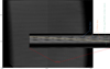 |
Fig. 1 Example of a darkfield corrected MiHI frame of a spatially featureless solar scene, obtained by averaging a large number of frames recorded at many different positions near the center of the solar disk. The image contains 5120 × 3840 pixels, the inset, highlighting the area in the red box, shows the individual spectra, packed onto the detector. The spectral direction runs from the upper left to the lower right, at an angle of approximately 3°, the boundaries of an example region containing a single spectrum are indicated by the yellow dashed lines. Spectral features belonging to adjacent image elements are separated horizontally. The image has two clearly visible brightness levels, the right half appearing systematically darker than the left one, a consequence of the uncorrected nonuniform gain of the camera. |
2.1 Coordinate mapping
The format in which MiHI data are projected onto the detector requires the determination of a coordinate map that connects each point and wavelength in the (x, y, λ) cube of interest to a location on the detector, the pixel association map (Pavlov et al. 2008). The determination of this map starts with the identification of at least some points on the sensor of which the spatial and spectral coordinate can be unambiguously identified with confidence, after which the missing coordinates can be filled in by means of interpolation.
Traditionally, this task is accomplished by offering the instrument light with known spectral characteristics, in the form of emission features from an arc lamp (Bacon et al. 2001) or from several monochromatic light sources (Pavlov et al. 2008). Such a spectral calibration is not usually done for solar spectroscopic observations. Instead, a reference spectrum is acquired by averaging a large number of frames near the center of the solar disc. The resulting spectrum, when averaged over a sufficiently large area, can be accurately described with a standard reference spectrum (Allende Prieto et al. 2004; Pereira et al. 2009), that was found to show little to no variability across the solar cycle at least for the photospheric lines (Livingston et al. 2007; Doerr et al. 2016). This reference spectrum is available at a high spectral resolution (R ≈ 500 000) and on an absolute wavelength scale (Delbouille et al. 1973; Neckel 1999). Since the prototype has not been stabilized in any way, and the image that is projected onto the detector is slowly moving, such an auto-calibration strategy is preferable since it offers the opportunity to recalibrate regularly.
We thus attempt to determine the coordinate maps by detecting spectral features in the flatfield image. Unfortunately, the intensity variations within each spectrum are not dominated by the spectral lines in the solar spectrum, but rather by the fringes of a moiré pattern, resulting from the sampling of one periodic structure (the regularly spaced, but tilted, spectra), with another one (the pixel grid of the detector). Although it is not possible to eliminate this effect completely, it has an amplitude that is directly proportional to the density of sampling of the focal plane (i.e. the pixel size of the detector). For critical sampling of the instrument focal plane, the amplitude is only a few percent, and can barely be noticed. If the data are significantly undersampled, however, as is the case in the MiHI detector plane, the ratio of the maximum to the minimum intensity increases to approximately a factor 2, leading to a variable pattern of fringes with an amplitude of around 30% of the mean, and a frequency that is usually dominating over that of the spectral lines in the selected passband.
Moiré patterns are highly sensitive to the relative position and angle between the two interfering patterns, and the phase of the pattern becomes particularly sensitive to the position of the image on the detector when the spectral direction is close to coaligned with the pixel grid. To minimize this sensitivity to the position of the image, the camera was rotated such that each image row is approximately coaligned with the pixel grid of the detector, so that the FOV of the instrument is approximately rectangular, and the angle between the spectra and the pixel rows is around 3°, which is large enough to limit the sensitivity to position changes to an acceptable level.
Fortunately, in ground-based data, the solar spectrum in many passbands is contaminated by a number of telluric lines, produced by radiative transitions of the molecules that comprise the Earth’s atmosphere. These lines are much narrower than solar lines, due to the low temperature of the Earth’s atmosphere, show none of the characteristic Doppler induced spatial variations that solar lines do, and their strengths are dependent on the amount of atmosphere that is present between the telescope and the Sun, and thus on the time of day at which the spectra are recorded. This last property can be conveniently exploited by recording a flat-field image at the center of the solar disc, but at different solar elevation angles. In the usual case that, apart from a small Doppler shift due to the rotation of the Earth, the solar spectra are very nearly identical, these flat-field images differ predominantly by the strength of the telluric lines, and the ratio of two such images therefore is dominated by a set of sharp, point-like features, marking out specific x, y, λ coordinates in the spatio-spectral domain, as shown in Fig. 2. These point sources can be readily located and identified, after which the path of the spectra can be described fairly accurately with a first or second order polynomial, fitted to the points belonging to a given microlens element.
Already for the MLA used in the prototype, the number of image elements is so large, that the only practical way to identify the telluric features is using an automatic detection algorithm. This is made challenging by variations in the optical performance of the instrument, and a number of imperfections in the MLA itself, resulting in a strong weakening or even the complete absence of some of the image elements from the data. To deal with these missing reference points, the raw image is first divided in bands that are approximately aligned with the grid of the MLA. Each band can therefore only contain light coming from one row of the MLA, of which the number of image elements is known. If the number of a specific spectral feature in a row corresponds exactly to the known row length, the row is assumed to be complete, and each feature can be associated uniquely with a particular image element.
To deal with the high density of telluric lines in some of the spectral passbands, the unambiguous identification of the particular telluric line that a specific spectral feature corresponds to can be difficult without a fairly accurate prior estimate of the path that is traced out by each spectrum. To obtain sufficient information to successfully complete this task, each image row of spectra (horizontal bright bands in Fig. 1) is extracted and de-stretched such that the dark band separating each image row from the next is aligned with the x axis of the new (curved) coordinates. The de-stretched rows are then divided into a fixed grid of rows and columns, and the number of spectral features in each of them is counted, thus resulting in a 2D histogram. Because the spectral direction is closely aligned with the x axis, if each image row is accurately de-stretched, the corresponding 2D histogram shows a horizontal band with a high density of spectral features for each telluric line in the passband. However, although several bands are clearly visible in the two examples shown in Fig. 3, none of them are straight and horizontal, suggesting that the initial detection of the row positions in the raw image was not extremely accurate.
The solution to this problem is to fit a polynomial to each band in the 2D histogram, and use that to produce a trace of the position of each telluric line on the detector. These traces are then extended upward and downward, forming an upper and a lower boundary, between which each detected spectral feature can be attributed to a specific telluric line. If multiple telluric lines are so closely spaced that the initial approximate trace was still insufficiently accurate to separate them, the subset of points between the upper and lower boundaries are a mixture of all of them. In such cases, the accuracy of the trace must be further improved. This is done by selecting the positions of all the telluric lines in the subset, and fitting a new trace to them, as shown in Fig. 4. In the most common case that only two telluric lines are present in the selection, the trace fitted to these points will usually separate the subset in it’s constituent subsets, as can clearly see in the bottom two sets of points in the figure.
Cross-checks, such as checking for approximate equidistant spacing of the spectral features, ensures that false, spurious identifications in the presence of missing reference points can be detected and removed. Every telluric line in each row for which that specific line is found to be “complete”, is now assigned a specific horizontal image coordinate, thus placing it at a unique position in the (x, y, λ) cube. Once a sufficient number of rows has been labeled in this way, a polynomial can be fitted to the positions that are known, thus allowing the approximate positions of all other (x, y, λ) coordinates to be interpolated.
In a subsequent step, the polynomial coefficients are refined and optimized, using a metric consisting of the sum of the squared distance of each “predicted” telluric line position to the nearest measured telluric line position, as long as they are sufficiently close. For the optimization, a steepest descent approach is used, that calculates the derivative of the metric with respect to all polynomial coefficients using a finite difference scheme. All lines for which no spectral feature could be found in the raw data within a radius of half of the calculated grid spacing are excluded from the metric and thus from the optimization, the mapped positions of these coordinates is thus based purely on interpolation.
Once at least two spectral features, for which the precise wavelengths are known, have been mapped in this way, all other wavelengths are calculated by interpolation of the spectral path using a first or second order polynomial, depending on the number of telluric lines available in the spectral range. The order of the fit is deliberately kept low, because the number of telluric lines is generally limited to just a few, the location of the telluric lines cannot be determined with infinite precision, and the wavelength of the telluric lines is not always known with very high precision. The combination of these issues can cause significant overshoot, so that fitting a high order polynomial here is best avoided.
The appropriate spectral sampling of the data along the path described by the polynomial depends on the width of the spectral PSF, the pixel size of the detector, and the angle of the spectrum with respect to the detector grid. To ensure that the individual spectra have as little overlap as possible, while fitting as much information on the image sensor as possible, the pixel size was deliberately chosen to undersample the focal plane by a factor of approximately two. Although sampling the spectra with a density higher than the pixel density projected onto the path is certainly possible, it yields no additional information, and is therefore best avoided. A sampling consistent with the size of a detector pixel projected onto the fitted polynomials is therefore optimal.
Because the dispersion depends on a combination of the grating angle and the field angle, and is not constant across the FOV, an optimal grid would result in a nonuniform wavelength grid across the FOV. To avoid this, a uniform wavelength grid was used that samples the spectra optimally when averaged over the FOV. This yielded approximately 588 wavelength points over the spectral range where the prefilter has a transmission of more than 5% anywhere in the FOV, and a wavelength step size of 10.0m Å.
This is in good agreement with the design target of the MLA (Paper I), that was dimensioned to provide a scale factor N of 16.9. Since the dark space available for dispersed spectral information scales proportional to N2, this should provide space on the detector for 285 spectral elements, that must be sampled by at least 571 points in the spectral direction.
Once the location of every point in the 3D cube on the detector is known, we can extract the image values at these locations to obtain a hyperspectral data cube. Since the data coordinates are not integers, and the spectra are inclined significantly with respect to the pixel rows, it makes no sense to extract pixel values directly, and values are extracted from the map by interpolation instead. Figure 5 shows an example of a raw data frame covering the spectral region from 5892.6 to 5896.8 Å, transformed to a 3D data cube by interpolation of the image to the appropriate coordinate map. The moiré interference fringes discussed above are transformed to an intriguing 3D pattern, that is not strictly periodic, and therefore in general does not have a sparse Fourier transform, so that it cannot be filtered out easily. Ignoring the spectral crosstalk in the extraction, results in parasitic spectral lines in the extracted spectra at wavelengths where no lines should be visible in the solar spectrum, and reduces the depth of the spectral lines, by contaminating them with the continuum from the neighboring spectra. Since the Na Dl line, contained in the spectral band shown in Fig. 5, has one of the lowest core intensities of any line in the solar spectrum at only 5% of the continuum intensity, it is a sensitive indicator of straylight contamination. Ignoring the transmission profile of the prefilter, the measured core intensity of 22% of the maximum intensity suggests a straylight contribution of at least 15%. Clearly, a description of the instrument with only a simplistic mapping operator is far from adequate, and a more complete description of the instrumental properties is required.
 |
Fig. 2 Example section of the ratio of a flat-field image, divided by another flat-field image recorded at a different solar elevation, for a 4 Å passband around 6302 Å. The blue dotted lines are the separation lines between the different rows of the MLA, the bright dots between the lines are produced by a pair of molecular O2 lines in this passband. |
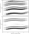 |
Fig. 3 2D histograms of the spectral feature density for one row of image elements for the spectral band at 589 nm (top) and the band at 656 nm (bottom). The grayscale indicates the point density as a function of normalized vertical coordinate (y axis), and horizontal position bin (x axis). Each dark band represents one or more telluric lines, with the bottom two bands of the top panel and the bottom band of the bottom panel containing two telluric lines each. |
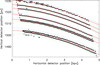 |
Fig. 4 Spectral features (black diamonds) produced on the detector by telluric lines in the spectral band between 5894 A and 5898 A, for one of the central rows of image elements. The solid red lines are fits to the high-density bands in Fig. 3, and accurately follow the positions of the spectral features on the detector. All spectral features located within a band around each red line (i.e. the area between the blue and green dashed lines) can be identified as resulting from a specific telluric line. Pairs of lines that cannot always be separated in the histograms (i.e. the lowest two bands in upper panel of Fig. 3) can now easily be separated and identified. |
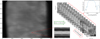 |
Fig. 5 Example of a raw MiHI data frame, recorded in the spectral region from 5891 to 5897 Å, containing a Ni line at 5892.7 Å, and the Na D1 line at 5895.9 Å, mapped to a 3D hyperspectral cube using the pixel association map only. The interpolation of the darkfield corrected raw image (left) to a series of monochromatic images (diagonal) also maps the moiré pattern, leading to a quasi-periodic fringe pattern in the monochromatic images. The spectrum, averaged over the FOV, shows clear signs of spectral crosstalk, manifesting as parasitic spectral lines, highlighted by the black arrows in the plot of the average spectrum (top right). The core intensity of the Na D1 line, that should be approximately 5% of the continuum intensity, is nearly 22%, suggesting that in this spectral band approximately 15% of the extracted intensity is coming from the neighboring spectra. |
2.2 Modeling the transfer map
To model the image formed on the detector of the MiHI prototype in full detail, it is not sufficient to consider the coordinate map only, we need to know the full spatial distribution of the monochromatic light that passes though one image element onto the detector. While, strictly speaking, this is the convolved image of the area of the object sampled by the MLA, we, from here on, refer to it simply as the PSF of the instrument.
The description of the contributions of the signal I′(u, v, λ) to the data values d(x, y) is formally described by the mapping operator M(x, y, u, v, λ), that describes for each point (x, y) on the detector how much light it receives from a given (u, v, λ) coordinate in the object plane. The total contribution to the data from an object area bounded by ul, uh, vl; and vh, spanning the wavelength range from λ − δλ/2 to λ + δλ/2, can thus be obtained by integration

If we can assume that the object intensity is constant within each MLA element of size l × l, we may perform the integral over u and v, resulting in the discrete form

where  is the object intensity integrated over MLA element u, v, and the sum over u and v is over all the image elements in the MLA. This expression is still a continuous function of the wavelength and detector coordinates, because the dispersion is continuous.
Although the mapping operator is a continuous function of the wavelength and detector coordinates, it can be converted into a fully discretized form by defining a wavelength grid and carrying out the integration over wavelength and detector pixels. To accomplish this, a complete and accurate description of the PSF is required, as a function of x and y. Since this description needs to include integration over the sampled object area and the optical imperfections of the individual MLA elements, it must in practice be obtained by numerical means on a discrete grid. We therefore proceed by considering each element of a properly resolved but discretized PSF φu,v,λ, as it is dispersed continuously across the detector pixels between the limits of the wavelength grid.
Modeling this process using a physical description of the instrument would present an excellent way to evaluate and optimize the optical configuration of the instrument. However, for the purpose of producing an accurate data formation model of the instrument, a more ad hoc description of the instrumental optical properties with polynomial approximations of sufficient order should suffice. The reduction in the complexity and speed of the optimization procedure that this approximate treatment affords when fitting the model to real data are so significant, that at present we cannot afford to ignore it.
We assume that within each wavelength bin the PSF is not wavelength dependent, and that each PSF pixel of size δ × δ is dispersed along a linear path Cx,y(t) = mx,yt + cx,y, so that the upper and lower limits of each PSF pixel for a given path coordinate t are given by

and

If we further assume that the efficiency of conversion of the incoming light to charge in each pixel is described by the continuous function ϒx,y(x′, y′), then for a given pixel (i, j) of a PSF φu,v,λ belonging to object pixel (u, v) and wavelength bin λ, the contribution to the signal detected in pixel (x, y),  , can be written as
 (1)
(1)
where the limits of the path coordinate tl and th are given by the section of the path for a given wavelength bin for which the associated  has an area of overlap with the active area of the pixel. Although at this point, the description for Iu,v(t) is still arbitrary, if we wish to fit that description to actual data values using an invertible operation, the only practical description for Iu,v(t) within each wavelength bin is of polynomial form, so that its coefficients can be brought before the integral and the integration can be carried out explicitly. We choose the simple polynomial form
  and obtain
 (2)
(2)
The total signal in each pixel due to the light in one wavelength bin of one MLA element, given by the sum over all PSF pixels

now has the linear form
 (3)
(3)
Although there is no fundamental reason requiring us to limit the polynomial order of Iu,v(t), the complexity of even a first order dependence on t comes at a significant numerical cost, and it is therefore not explored in this paper. We limit the order to 0, so that Iu,v,λ = k0, and  Neglecting the wavelength dependence of the intensity cannot be justified in any way, nonetheless, it is most likely a fairly accurate assumption for the high resolution data analyzed here. For data of lower spectral resolution, however, retaining higher order terms may well be required to obtain an accurate result.
We now focus our attention on the evaluation of Eq. (2). There are in total 10 ways in which  can overlap with a detector pixel: full overlap, no overlap and overlap that is limited in the x and/or y coordinate on the upper or lower spatial integration limits. To calculate what signal is actually detected by a specific detector pixel x, y, we must therefore decompose the path in sections for which the overlap is of a specific type, and evaluate Eq. (2) using the appropriate integration limits.
Figure 6 shows an example of such a multisegmented path, covering four different types of overlap. The calculation proceeds by detecting the borders between the different types, indicated by t0 … t4, evaluating the appropriate expression for each segment, and adding up the contributions.
To evaluate Eq. (2) for each segment, a description for ϒx,y(x′, y′, t) must first be given. For detectors that have a filling factor of unity, it can simply be set to 1, reducing the integrals to their simplest possible form. Unfortunately, for modern CMOS sensors, the use of microlenses to enhance the quantum efficiency is widespread. This leads to a position dependence of ϒx,y(x′, y′, t), caused by microstructures on the pixel surface and optical diffraction effects in the microlenses, that can even be dependent on the properties incoming beam. In practice, the only tractable solution is a simplified description based on basic arguments, which will be discussed in more detail below.
To carry out a classical optimization, derivatives of the detector signal to each of the model parameters that is to be optimized are usually a very effective way to improve numerical performance. With the expressions at hand, these derivatives are readily calculated, by analytically taking the derivative of Eq. (2) with respect to each desired variable. All derivatives of the path coefficients can ultimately be expressed in terms of the derivatives in the PSF coordinates x and y, whereas all derivatives with respect to the PSF parameters can be obtained by calculating the derivatives of the PSF with respect to each parameter using a finite difference approximation, and evaluating Eq. (2) for each pixel of the PSF derivative. Since the PSF appears in front of the integral, these results can be obtained without additional cost. A full description of the expressions for the different types of overlap for a constant I(t), and their derivatives, is given in Appendix B.
We proceed by formulating a partially parameterized description for M, that includes as much information as possible of the real instrument. We start by calculating the properties of the light emerging from the MLA, based purely on theory, and model the remaining properties of the instrument and the detector using a simplified ad hoc polynomial description.
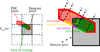 |
Fig. 6 Example of a path integral of the area of overlap of one PSF pixel. Left: overview of an area of 3 × 3 dector pixels, showing the area covered by a PSF pixel, dispersed over a spectral interval [t0 − t4] (red/green), and the detector pixel under consideration (gray). Right: detail showing the path, which is split up in four different segments. The types of overlap are: none (t0 − t1), top + left limited (t1 − t2), top limited (t2 − t3), and full overlap (t3 − t4). |
2.2.1 PSF model
The most important ingredient needed to construct a full transfer map for the MiHI prototype, that goes beyond the direct data extraction according to the pixel association map, is the monochromatic image of the front side of the MLA, as imaged onto the detector, after it was scaled by the MLA and passed through the spectrograph, the PSF φ from Sect. 2.2. To obtain this PSF, we can resort to a direct measurement using a monochromatic light source (e.g., Brandt et al. 2017; Berdeu et al. 2020), but such an approach is complicated by the high spectral resolution and high-density layout of the MiHI prototype. For a reliable measurement, the light source must be monochromatic compared to the spectral resolution of the instrument and sufficiently bright to still be detectable with the image sensor, a combination that at R = 300 000 can only be achieved using a LASER source. Unfortunately, light produced by LASER sources is fully coherent, so that the PSFs of the individual MLA elements may not overlap, or interference effects will destroy the reliability of the measurement. Faced with the high-density layout of the MiHI prototype, this approach was therefore not favored.
To proceed, we obtain the PSF by modeling and fitting a simplified description of the PSF to data obtained with the instrument instead. Such an approach was used by e.g. Bacon et al. (2001), who combined a detailed description of the optical layout of their instrument, supplemented with local measurements, to obtain individual cross-dispersion profiles for each of their spectra. Here, we follow an approach more akin to MFBD wavefront sensing (Löfdahl & Scharmer 1994; van Noort et al. 2005), and model the PSF as resulting from wavefront phase errors, that are described using Zernike polynomials. Although such a model of the PSF is inevitably more approximate then a direct measurement, it allows for the fitting of the wings of the PSF, something that is difficult to measure directly due to the limited dynamic range of most image sensors, but which may be responsible for a significant fraction of the instrumental stray-light.
In Paper I, we modeled the imaging properties of the doublesided MLA using a numerical code, that calculates the stationary propagation of the electric field through the MLA using Huygens principle. From this, intensity and phase distribution maps could be calculated in planes located inside and behind the MLA. Such maps must now be obtained for a realistic configuration of the actual MLA that was used in the prototype, and allow for small but significant deviations of the lens radii and positions, as one would expect from a physically realistic device. We also want to take into account the opening angle of the telecentric input beam, which is responsible for a small amount of broadening of the PSF of the MLA.
To obtain such maps, it is not sufficient to simply propagate the light emerging from the ideal model, and pass it through a model of the spectrograph, since this would ignore the individual errors originating in the individual MLA elements entirely. Since we lack detailed physical measurements of the properties of the individual elements in the MLA, we also cannot model the propagation through them explicitly. We therefore take the electric field distribution of the light emerging from the ideal model from Paper I, and propagate it to the pupil plane of the spectrograph, where we impose an additional wavefront phase error that describes the changes resulting from the propagation through the real MLA element, as well as changes resulting from propagation through the spectrograph.
To facilitate the calculations that follow, it is most practical to obtain the electric field in the pupil on a grid with a spacing that transforms to a multiple of the pixel size in the detector plane. However, this is easier said than done, since the optical system between the grating and the detector is not free of image distortions, so that there is no unique value for the grid spacing that satisfies this constraint.
Here, we settle for a compromised value for the grid spacing, shown in Fig. 7, and assume a uniform image scale across the detector. A deviation of the true pixel scale from the compromised value is in principle equivalent to a scale change in the PSF, however, we assume that this scale change can be described accurately with an appropriate phase error of the electric field distribution in the pupil plane of the spectrograph.
Because the MLA is a diffraction dominated device, the effect of propagation through the MLA is expected to be minor compared to the effects of the pupil apodization caused by diffraction. However, optical aberrations of the instrument itself are not negligible, and the imprint they leave on the PSF of an individual image element depends to some extent on the path that the light takes through the instrument. These instrumental aberrations themselves may be smoothly distributed across the FOV, however, there is no reason to assume that the uncorrelated alignment error within the MLA is also smooth. This implies that it is perfectly plausible that the variation of the PSF across the FOV is not smooth at all, because it is an ensemble of randomly selected samples from a smooth distribution. In the final model, we therefore only encourage smoothness of the aberrations, by means of repeated reinitialization with a smoothed start condition, but we do not strictly enforce it, so that the individuality of the PSF of each MLA element can be captured. The more elegant method of adding a penalty function to the optimization metric for departures of the PSF from smooth behavior was not tested.
We assume that the order of the aberrations for each MLA element is low, partly because the effect of diffraction is assumed to be dominant, but predominantly inspired by the numerical effort required for including high order aberrations. High order aberrations cannot be excluded entirely though, because the far wings of the PSF contribute significantly to the stray-light and the spectral cross-contamination in the raw data. Therefore, a limited number of modes of high radial order but low angular order was included.
 |
Fig. 7 Electric field amplitude (left) and phase (right) in the output pupil of a single MLA element, on the compromised computational grid. The zeroed out area around the illuminated part of the pupil, needed to obtain an oversampled PSF is clipped. |
2.2.2 Map coordinates
In Sect. 2.1, a method for the determination of the basic mapping of the data coordinates (u,v,λ) onto the detector array coordinates (x, y) was described, based on the detection of telluric lines in the spectra. However, even if the coordinate map is accurate, the specific location where a demagnified monochromatic image of the MLA entrance lens falls on the detector is only a very crude description of the spatially extended distribution of the light on the detector, and it is used here only as a point of reference for the actual spatial distribution map.
For optimizing the full transfer map, the coordinates cannot be constrained by the telluric lines, since these are varying in time and there is no way of knowing exactly where and how strong they are for a given dataset. Instead, the coordinates are constrained by trying to match the intensity distribution on the detector, perpendicular to the spectral direction, at all wavelengths in the spectral range. We use a similar approach as in Sect. 2.1, and describe the detector coordinates (x, y) with polynomials in the wavelength λ
 (4)
(4)
where px,u,v,n and py,u,v,m are the polynomial coefficients for each MLA element (u, v) in the x and the y directions respectively. To achieve a sufficiently accurate description of the spectral path, the order of the polynomial must be taken considerably higher than 2 in at least one dimension. To obtain the local, linear description Cx,y of this curve, which is needed to evaluate Eq. (1), we approximate the spectral path locally with its tangent.
Unfortunately, describing the path coordinates as a function of λ implies that the length of that path between two wavelength limits must equal the dispersion  integrated between those wavelength limits. This condition is satisfied when
 (5)
(5)
which imposes a non-linear constraint on the polynomial coefficients that is difficult to impose during the optimization.
For the data of the MiHI prototype, the dispersion direction is relatively closely aligned with the horizontal detector coordinate, therefore, the order of x(λ) can be kept linear without much loss of accuracy. If we further assume that the coefficients for y(λ) are much smaller than those of x(λ), which can be justified by the small angle of inclination of the dispersion direction with the x axis, we can satisfy Eq. (5) fairly accurately by imposing a linear constraint only on px,u,v,1, which defines the dispersion. For configurations where such approximations cannot be made, an additional polynomial description of the wavelength as a function of an independent path coordinate may be required, which may be difficult to constrain.
2.2.3 Detector response
One of the major challenges in constructing a solar integral field instrument is finding an image sensor that is large enough to critically sample all the information generated by the instrument, and at a frame rate that is sufficiently high to allow for image restoration of the recorded data. Development of such image sensors has made remarkable progress in recent years, so that at present cameras with an image sensor of 20 Mpx and more are readily available, that can capture 30 full frames per second, and with a readout noise of less than 8e– rms (e.g., Fowler 2006).
This kind of performance can be achieved with a modern CMOS sensor, when complemented by massively parallel readout electronics, all of which is integrated onto the sensor die (see e.g. El-Desouki et al. 2009, for an overview). Such integration can come at the price of significant imperfections in the signal processing, such as a non-linear intensity response, [strong] nonuniformities in the detector gain, and, in some cases, even crosstalk between different sensor areas (Li et al. 2002; Dieter et al. 2020).
Linearity
For the work presented here, we only attempted to calibrate for the global nonlinearity of the sensor, common to all pixels. To measure this, the sensor was illuminated as homogeneously as possible using a LED, through which the current is controlled accurately, and which can be switched on and off much faster than the camera exposure time. This LED was placed in the focal point of a lens, generating a collimated beam, which was used to illuminate the sensor, resulting in an relatively homogeneous light distribution. By illuminating the sensor with pulses of light with a precisely controlled width, the linearity of the response of the camera can be measured. Figure 8 shows the measured response of the CMOSIS CMV20000 sensor, on which the cameras are based, as a function of light level, coplotted with a linear response curve. Clearly, the departure from a linear response is quite significant, especially for a low signal level, and must be taken into account in the data reduction to obtain accurate line profiles.
Describing the response of the entire detector with a single response curve is arguably very crude, especially if the homogeneity of the light distribution on the sensor used to obtain it was not of the highest level. However, since the global non-linearity was found to be minor compared to the effect of the pixel filling factor described below, we corrected the synthetic images generated by the forward model only in this crude, global way. The full, pixel specific form of the non-linear response is a complicated function of the intensity distribution on the entire sensor area, and is still the subject of further calibration efforts.
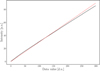 |
Fig. 8 Response of a CMV20000 CMOS image sensor, averaged over the entire area (black), compared to a linear response (red-dotted line). |
Filling factor
Because the detector used in the prototype is a front-side illuminated CMOS sensor, there is a significant fraction of the sensor that is insensitive to light. The sensor therefore has microlenses placed directly on the pixel array, to focus more light on the light sensitive area, thus enhancing the total quantum efficiency (QE). Despite these microlenses, the QE of the sensor is rated at not more than 0.65, indicating that a significant fraction of the light is still lost.
We could describe this effect in terms of the pixel response function ϒx,y(x′, y′) but lack a detailed description. Instead, we assume that the response of the pixel is uniform, except for the loss of light, which occurs primarily on the edges of the pixels, where the microlenses are butted together. Based on basic principles of diffraction, the width of the boundary zone, B, over which the surface discontinuity formed by the boundary between two microlenses affects the propagation of light, is on the order of one wavelength. Instead of adopting an ad hoc description for ϒx,y(x′, y′) in this area, which would lead to more complex and time consuming expressions for the path integrals, we assume that the light in this area is lost completely, because it is diffracted onto the light-insensitive parts of the sensor. The pixel gain map then reduces to
 (6)
(6)
This, in effect, approximates the effect of the microlens boundaries by reducing the effective pixel size, while leaving dark, light insensitive bands in between. For a wavelength of approximately 0.5 µm, and a pixel size of 4.7 µm, we would thus expect these diffraction effects to reduce each pixel dimension by approximately 10–15%.
As a consequence, the drop in signal that ensues when a spectrum crosses over from one pixel line to the next, purely due to the change of the distribution of the charges from one to two pixel rows, is increased by the amount of light that is completely lost in the boundaries of the microlenses. The effect is an enhancement of the moiré fringe pattern in the raw data, that mimics a severely non-linear detector response, but that cannot be explained by an actual non-linearity without severely affecting the inferred depth of the spectral lines.
Assuming that this effect is symmetric in the x and the y directions, the value of the optimal fit to the pixel size is ±0.43 of the pixel pitch, in good agreement with the expected 10–15% reduction estimated above. Consequently, approximately 26% of the light is lost on purely geometric grounds, which, when compounded by reflective losses, appears to be roughly compatible with the peak QE of 0.65.
2.3 Optimization of the model parameters
We now proceed to fit a discretized map of the instrument transfer function to a flat-field frame: a frame that is obtained by averaging a large number (10 000) of randomly placed individual images, recorded near the center of the solar disc. Unlike a flat-field frame for an imaging instrument, this flat-field is anything but void of structure, because the image consists of individual spectra, separated by dark space, as shown in Fig. 1.
The aim is to reproduce this flat-field image by applying the transfer map to the true input spectral cube, and minimizing the difference by fitting the parameters that control the transfer map. Although the forward model consists of a well-defined, if approximate, procedure, due to the high contrast in the image, the simulated image must be very accurate to obtain a meaningful gain correction map. This can be considered an advantage, because it places strong constraints on some parts of the instrumental mapping function, but in practice it leads to limitations on the accuracy with which the flat-field image can be reproduced.
The input cube itself is not a priori known, since the exact transmission profile of the prefilter is not known, and the depths and positions of the telluric lines are varying continuously. In practice, we therefore need to already know the transfer map and apply it to the flat-field image to gain knowledge of the input spectral cube. However, any error in the transfer map will lead to an error in the recovered spectral cube, which cannot be definitively attributed to either the map or the true input spectrum. This entanglement of the model and the input spectrum is handled iteratively by interlacing the extraction and regularization of the input spectrum with each optimization step of the model parameters, as outlined in Fig. A.1.
Significant regularizations must generally be imposed on the input spectral cube, to differentiate between fit errors caused by variations in the gain map, those arising from errors in the instrumental mapping function, and those caused by errors in the assumed input spectrum. The most important regularization steps applied to the data are outlined in Sect. 2.3.2.
The well known Levenberg-Marquardt optimization algorithm (Levenberg 1944; Marquardt 1968), that uses the forward model and its derivatives, was used to minimize the difference between the artificial image, generated with the regularized spectral input cube, and the observed flat-field image. Because the spectra are packed closely together on the detector in one direction, there is significant overlap of the spectra in that direction, which causes coupling between the fit parameters of the individual image elements in that direction. In the other direction, in which the prefilter divides the image in dark and bright bands, there is also overlap between the spectra, but it is only significant in the extremes of the spectral range. If the variation of the fit parameters is constrained to be of a simple form across the entire spectral range, the resulting coupling of the fit parameters caused by the latter overlap is negligible, and the Hessian has an approximately block-diagonal form. The small amount of coupling that does exist between the blocks can be adequately handled iteratively, allowing for the Hessian to be considered truly block-diagonal, which greatly reduces the effort required to invert it.
2.3.1 Data extraction
To extract the hyperspectral data cube V from the data values d, we need to obtain the inverse of the instrumental transfer map M. Using the framework of generalized least squares regression, an estimate of the data cube can be obtained by solving

where the weighting matrix W is typically defined as the inverse of the dispersion matrix ∑ of the data points, which describes the estimated distribution of the data values around their means (see for example Rothenberg 1984, and references therein), but can be adjusted to weight data values also on other grounds, or even eliminate data values altogether. Although the present data certainly contains its fair share of pixels of variable fidelity, the vast majority of these pixels are not actually bad, but exhibit a rather non-uniform, non-linear intensity response, so that estimating W is not straightforward. Therefore, no weighting was applied, allowing this behavior to propagate to the hyperspectral data cubes, where it was eliminated in a process described in Paper III. We thus omit W, proceed with the expression for an ordinary least squares (OLS) fit to the data
 (7)
(7)
and attempt to invert the operator on the left hand side (LHS) somehow. Unfortunately, although ℳ is sparse, so that ℳTℳ is sparse, and can be stored in just a few GB, the inverse is not sparse, and would require the full operator of Ncube × Ncube = (128 × 114 × 588)2 elements to be explicitly stored somehow. Since an affordable computer that can store 7.3 × 10¹³ floating point values in RAM will likely remain a thing of the future for some time to come, an alternative method to obtain the solution of Eq. (7) is required.
We resort to an iterative scheme, by subtracting the result of the application of ℳ to a trial solution ℳ𝒱n = dn from the observed data d. We multiply with ℳT and use the linearity of ℳTℳ to write
 (8)
(8)
We now solve repeatedly for the corrections qn by approximating ℳTℳ by a form that captures its essence, while being simple (cheap) to invert. Using the cheapest such approximations, the diagonal, the solution converges rapidly, as shown in Fig. 9. The convergence rate can likely still be improved by using a step optimization method (e.g. conjugate gradient, BFGS, etc.), but from the behavior, a reduction of 6 orders of magnitude, the precision limit of a single precision floating point number, is achieved in the RMS value of the defect after only 50 iterations.
Unfortunately, although the operator ℳTℳ is sparse, due to the partial overlap of the extreme ends of the spectral range between adjacent rows of the MLA, it is not compact, with on average approximately 500 values spread over large parts of the index range for each row. This makes storing it awkward, and calculating it takes a significant amount of computing time. This is problematic, since ℳ is continuously changing during the optimization, which requires ℳTℳ to be recomputed for each optimization step, thus dominating the computational costs of the optimization procedure.
We therefore turn to an alternative method that can be used to solve
 (9)
(9)
directly. Since in this formulation the data are not fitted in an optimal way, the method may be more vulnerable to degeneracies, numerical instability, noise and bad pixels. If these problems can be managed successfully, however, the method promises to be at least two orders of magnitude faster than using Eq. (8).
Since the right hand side (RHS) of the problem is specified in image coordinates and not in cube coordinates, a physically intuitive approximation to the inverse exists that is both accurate and cheap: the pixel association map. In Sect. 2.1, an approximate pixel association map was determined using telluric lines, containing for every (u, v, λ) point in the data cube the x and y coordinates on the detector where the value of that data cube entry is located. Since these locations are not integers, the data values must be obtained by means of interpolation. The interpolated data cube completely ignores the spatial smearing by the instrumental PSF, however, this is not different from approximating ℳTℳ with its diagonal.
We thus modify 𝒱n not by approximating ℳ directly, but by interpolating the defect image βn in the pixel association map coordinates xp and yp
 (10)
(10)
where Ipol represents the interpolation operation. We use qn to correct 𝒱n
 (11)
(11)
and iterate Eq. (9) to Eq. (11) until convergence is achieved.
Figure 9 shows the residual as a function of iteration number. The solution initially converges rapidly, but to an RMS value that is considerably larger than for the method that uses Eq. (8), because the RHS has not been filtered by multiplication with ℳT. After the initial convergence, a plateau phase can be seen, in which convergence appears to have been achieved. Unfortunately, there is a component in the solution, that is able to grow exponentially and eventually overwhelm the solution, causing the residual to diverge exponentially after a few hundred iterations.
Extensive testing suggests that the growth rate of the parasitic component is related to a particularly unfortunate sampling of the image plane, in regions where the distance between spectral samples is very close to one pixel. In such cases, it is possible to sample the detector plane over a significant spectral range very close to the pixel boundaries, causing the sum of two extracted values to be constrained, but not their individual values, allowing for an unconstrained oscillatory solution to grow without bounds. Because the dispersion is not uniform across the FOV, if the spectral sampling is chosen to be close to one detector pixel, this condition is nearly always satisfied in some fraction of the FOV.
Although the issue could be prevented by changing the spectral sampling density so that it is larger than one pixel everywhere, or by changing the sample locations for each image element to be centered on the image pixels as much as possible, this would compromise the homogeneity and/or information content of the extracted data cubes. There is, however, no indication that this component has a significant amplitude until well after the hyperspectral data cube has converged, so that a timely truncation of the scheme appears to present an acceptable way to mitigate the problem. For typical application to the prototype data, 15–25 iterations appears to be a good compromise, therefore, we consider this method converged after 15 iterations.
A comparison of the convergence behavior of the residual using the two methods in Fig. 9 suggests that although the OLS based method initially converges somewhat slower, it appears to have superior stability. A direct comparison of two data cubes, extracted from the same raw data frame with 15 iteration of the interpolation based method and with 50 iterations of the OLS based method, is shown in Figs. 10 and 11. Especially in Fig. 11, it is clear that the recovered data cube contains the same information, even the photon noise is nearly identical, but some small differences can nonetheless be observed. The RMS amplitude of the relative difference between the two solutions is around 1.5% in the continuum, which is more than 3 times smaller than the photon noise in the data, and shows no significant structure related to the content of the extracted cube. The cost of obtaining the interpolation-based solution is, however, more than two orders of magnitude lower, which is why it was selected for the optimization.
Although the selection of the interpolation based extraction method for the optimization can be entirely justified by the inevitable changes in M that occur during the optimization process, for science data M describes the known instrument properties, and should in principle be constant, provided the instrument response does not change. Therefore, although it could not be used in this paper, the OLS based extraction should be considered the method of choice for science data.
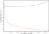 |
Fig. 9 Defect as a function of the iteration number for the interpolation based method (black) and the least squares fitting method (red). |
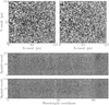 |
Fig. 10 Difference of two data cubes, extracted from the same raw data frame with the interpolation based method and with the OLS based method, normalized by the mean continuum value of both cubes. Top left: spatial cut at a wavelength coordinate of 200. Top right: spatial cut at a wavelength coordinate of 452. Middle: x − λ cut at y = 57. Bottom: y − λ cut at x = 63. The grayscale runs from −0.01 to 0.01 in all panels. |
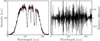 |
Fig. 11 Difference of two spectra, extracted from the same raw data frame with the interpolation based method and with the OLS based method. Left: spectrum of the direct method (black) and the least squares method (red). Right: difference between the spectra from the left panel. |
2.3.2 Spectral model
The process of modeling the input spectra is facilitated significantly by assuming from the very beginning that the input spectrum is identical to a high resolution reference solar spectrum, such as the FTS solar atlas by Neckel (1999). This assumption, however, is strictly speaking not correct, not because the solar spectrum is too variable, but because the transmission properties of the prefilter of the instrument vary significantly across the FOV. In addition, since neither the properties of the Earth’s atmosphere nor the line of sight velocity between the Sun and the Earth during the observations are identical to those during the recording of the reference spectrum, there are significant differences in the strengths and positions of the telluric lines in the spectral range.
We must therefore first adjust the strength and position of the telluric lines in the FTS reference spectrum, and reconstruct the input spectrum by multiplication of the adjusted reference spectrum with a fit to the prefilter curve, for each image element in the FOV. In doing so, any imprint of model imperfections and gain map variations on scales that are small compared to the adjustments is largely ignored, thus providing a much closer approximation to the real spectrum in each image element than the one obtained by direct extraction of the data cube from the flat-field image.
Fitting the prefilter transmission profile
For the characterization of most data, it is sufficiently accurate to assume that all image elements see the same spectrum, and this can be obtained by averaging over all spatial dimensions. In the case of the data of the prototype, however, this does not really work, because although the assumption that the solar spectrum is the same for all image elements is likely still valid, due to the steepness requirements on the prefilter, its transmission curve is varying significantly across the FOV.
To obtain the true input spectrum, we must therefore multiply the true solar spectrum with the transmission profile of the prefilter for each pixel. Unfortunately, this curve must first be fitted to the observed spectral cube.
To this end, we remove the solar lines from the spectrum of each pixel by dividing them by the normalized reference spectrum. In the likely case that the solar lines are Doppler shifted with respect to the spectral cube, the residual will have a positive and a negative lobe, which should not significantly affect the prefilter curve. To maximize the accuracy, we use the logarithm of the ratio of the extracted spectra and the reference spectrum as the data points for the prefilter fit, so that the exponential character of the curve near the edges can be accurately described.
An additional challenge comes from the overlap between adjacent image rows that makes it difficult to fit the wings of the prefilter explicitly, because they are always blended. The fit of the prefilter is therefore only carried out in the bright middle section, where overlap is not a significant issue, and the result is then extrapolated to the area of overlap.
Although the assumption that the spectra are well described by the reference spectrum is probably fairly accurate, the presence of telluric lines in the spectra leads to significant complications. This is, because in the frame of reference of the solar spectrum, these telluric lines are varying both in amplitude, due to the elevation angle of the telescope, and in wavelength, due to the line of sight (LOS) velocity of the telescope relative to the solar surface. The resulting mismatch in the spectra can be large, as can be seen in Fig. 12, in which the telluric lines have a different strength and position in the data then in the reference spectrum, causing a predominantly positive mismatch. Since the mismatch has a nonzero mean, it affects the fit of the prefilter, pulling it up near the edge, as can be seen from the deviation of the black curve from the data in the example shown.
We can proceed with the fit to the data points by excluding the range of the telluric lines, however, if the procedure for matching the telluric lines described below has been applied successfully, this is usually no longer needed.
We fit a 10th order polynomial to the remaining data points using a least squares fitting routine, and extrapolate the wings for a prefilter transmission below 50%. This cannot be done for each individual spectrum, since local gain variations and noise can have a severe impact on the accuracy of the fit, especially in the range that samples the prefilter wings. Since we expect the prefilter to exhibit only smooth spatial variations of the transmission curve, we instead fit a low order 2D polynomial to each of the prefilter coefficients.
While this works very well across the vast majority of the FOV, it generates significant overshoot problems in areas of large variations in the transmission, such as vignetted areas, especially when the blocking structures are not near focus. Such areas are therefore best avoided, either by eliminating them from the data set, or by adjusting the setup to avoid the vignetting altogether.
Finally, the prefilter curve is obtained from the exponential function of the fitted polynomial, and the spectral lines are reintroduced into the spectra by multiplication of the prefilter curve with the reference spectrum. We thus obtain a best effort approximation to the true input spectrum for each image element.
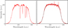 |
Fig. 12 Example of fitting the prefilter transmission curve. Left: raw extracted spectrum. Right: ratio of raw to reference spectrum (red) and the 10th order logarithmic fit (black). |
Adjusting the telluric lines
One particularly difficult aspect in using a terrestrial reference atlas to model a MiHI flat-field image is that the reference spectrum was recorded at a different geographic location, altitude, and time of day and year, from the current data. The LOS velocity between the telescope and the Sun depends not only on the time of day, but also on the time of year, and causes the absorption lines that originate in the Earth’s atmosphere (telluric lines) and the Solar spectral lines to shift in wavelength relative to each other. The optical thickness of the Earth’s atmosphere, a function of the elevation of the Sun above the horizon, the altitude of the telescope, and the specific weather conditions, determine the strength of the telluric lines in the observed spectrum. Unfortunately, the time of day when the strength of the telluric lines is minimal and the wavelength shift introduced by the rotation of the Earth is at its smallest, is also the time of day that the wavelength shift changes fastest, causing the lines to broaden if too much time is taken to record the flat-field images.
A poor match to the telluric lines may not seem like a huge problem, because even after excluding them, most of the spectral range remains available for constraining the instrumental transfer map. If the masking is carried out thoroughly, however, and includes the full extent of the instrumental transfer function, the close proximity of the neighboring spectra leads to an unacceptably large loss of data points. We therefore must find a way to model the telluric lines with sufficient accuracy so as not to influence the quality of the fitted model.
To obtain a good enough match to the true spectrum, we multiply for each image element the reference spectrum with its corresponding prefilter curve, and average that over the entire FOV. We then average the spectral cube extracted with the current instrumental map, scale appropriately, and take the difference with the averaged reference spectrum. If the instrument map is not very inaccurate, the differences between the spectra are dominated by the difference in the telluric lines, which is added to the reference spectrum in a small wavelength band around the approximate location of the telluric lines. By applying this procedure iteratively, the telluric lines in the reference spectrum can be made to resemble those in the flat-field data.
2.3.3 Wavelength coordinates
The goal of fitting a transfer map to the instrument is to convert the raw data to a 3D data cube. The wavelength coordinate of that data cube are, however, to some extent still arbitrary. We can identify three relevant frames of reference, that of the Sun, that of the Earth’s atmosphere, and that of the observatory. All three are present in the spectra, in the form of the solar lines, telluric lines and the prefilter curve respectively.
The decision which one to use for the map is not straightforward. Clearly, matching the reference spectrum and modifying the telluric lines to match those in the data selects the solar frame of reference. While this is the most desirable choice from the perspective of subsequent data analysis, this frame of reference moves on the detector during the day, due to the rotation of the Earth, thus causing fixed instrumental features to move during the day. Here, we settle for a hybrid solution, where the model is optimized to an observed flat-field frame and referenced to the solar frame at that time, for which the tellurics are modified accordingly. Any change of the solar wavelength reference during the day is then considered by adjusting the wavelength scale of the reference spectrum, so that fixed instrumental features remain fixed.
Although the reasons for it remain unclear, the L-M fit procedure that was used to optimize the polynomial coefficients that describe the spectral path, was not effective in adjusting the wavelength scale to any selected frame of reference. This problem can be addressed effectively by determining the wavelength scale and correcting it in a separate step. This was done by extracting the spectra, and matching them to the reference spectrum by adjusting the wavelength reference and the dispersion. The coefficients describing the path of the spectra on the detector were subsequently recalculated from the old ones using the coordinate transformation from the old wavelength coordinate to the new one, in effect a simple regridding of the spectral coordinates along the spectral path.
2.3.4 Scattered light
Thus far, we have only considered wavefront errors contributing to the PSF. However, the dispersive element of the instrument is a ruled Echelle grating, which is located near the pupil. The edges of the grating lines, even when they are executed perfectly, will scatter the light that falls on them in all directions, resulting in a spatially extended stray light contribution.
The intensity and scale of this stray light contribution depends on many factors, such as the roughness of the edges of the grating lines, the line profile, the coating material on the grating, etc., which makes it difficult to model it with any level of accuracy. Here, we manually fit a power law distribution of scattered light, only in the spectral direction, perpendicular to the grating lines. This scattering term is added to the PSF as a weak, constant term, so that it does not need to be considered in the calculation of the gradient of the PSF.
To calculate this term, we first calculate the slope md of the dispersion direction, which is tangential to the spectral path, and determine the line that is centered on the coordinates (xp, yp) of the maximum of the PSF, perpendicular to the dispersion direction. Assuming that the dispersion direction is closely aligned with the horizontal (x) axis, we can calculate the vertical displacement to this line for a horizontal displacement δx = (x − xp) from δy = mdδx. For each pixel of the map element ℳu,v,λ, we now calculate the distance in the dispersion direction for pixel (x, y) to the line going through xp, yp,

and determine the value of  by interpolation.
We multiply the maximum value of the PSF in the map for each pixel with a Cauchy-Lorentz distribution, and add it to the map
 (12)
(12)
where the aproximation was made that md is small, so that the interpolation of ℳu,v,λ in x can be neglected.
The values of γ and α need to be experimentally determined, by requiring that the wings of the spectral lines in the extracted hyperspectral cubes do not show a significant deviation from the lines in the reference spectrum. The values α = 2, and γ = 0.3 were found to reproduce the FeI lines at 6301.5 and 6302.5 Å satisfactorily, with no significant systematic fit errors visible in the residual across the entire spectral range.
In reality, the scattered light contribution consists also of scattering surfaces other than the grating, and this distribution is more symmetric, and extends sufficiently far from the center of the PSF to cover the entire spectral range. Although this would strictly speaking require the map elements to cover a significant part of the entire field of view, the extreme wings of the PSF blend with the wings of many other PSFs into a background contribution of scattered light, that retains virtually no image information whatsoever. To avoid the numerical difficulties of modeling this light explicitly, this global scattered light contribution is therefore assumed to be radially symmetric, and is removed prior to fitting the map. As before, the form of the scattering function is assumed to be of the Cauchy-Lorentz form

where  is the radial distance to the center (x0, y0) of the map element, and ξ and κ are determined experimentally by minimizing the mean value of the data in the dark areas of the FOV, where the width of the core of the PSF is kept well below a pixel, so that the PSF resembles the sum of a delta function and an extended wing contribution.
The images without the scattered light contribution can now in principle be calculated by a straightforward deconvolution of the raw data. However, since deconvolution is an expensive operation that is in addition sensitive to noise, it is advantageous to consider the core and the wing parts of the PSF separately.
If the PSF can be thought of as a delta function with extended wings, the convolution operation can be split in two additive contributions: an unmodified source term corresponding to the core, and a smooth background term corresponding to the wings.
Convolving the convolved image for a second time results in a doubling of the background contribution, in addition to a second order term consisting of the background contribution convolved again with the wings of the PSF. If the wings of the PSF are sufficiently weak, this term may be ignored, and a good approximation to the background contribution can be obtained from the difference between the raw and the convolved raw data frames, that can be subtracted from the raw frames, so that it need not be considered explicitly.
3 Results
Although the description above is kept deliberately as general as possible, so that it can be applied to an arbitrary wavelength band, it takes a significant amount of time and effort to arrive at a good fit for the map for a given wavelength band. Therefore, here, we focus on the results for the wavelength band of 6302 Å only, since it is centered at the design wavelength of the prototype optics, and the optical performance is therefore probably closest to optimal.
The model was optimized using the procedures described above, as outlined in Appendix A. The code performing the optimization was written in C++, and is roughly structured as outlined in Fig. A.1, but has many miscellaneous code fragments used for testing or to initialize or manipulate variables manually. Although it may evolve into a code for general calibration of solar IFS instruments eventually, it is currently not in a state that makes it suitable for general use. It is nonetheless made available as online material to the interested readers1.
Despite our best efforts to include all known details into this model, some simplifications needed to be introduced to keep the problem tractable. The PSF had to be limited to not more than 31 × 17 pixels, and the fitted parameters to less than 25, for which the calculation of the transfer map and its derivatives already required a total of more than 1TB of RAM and around 256 core hours to calculate. To make this tractable, the calculations were therefore distributed over 4 compute nodes and divided in 16 overlapping horizontal bands across the FOV.
The parameters of the scattering PSF for the 6302 Å spectral band for which the subtraction of the dark background and scattered light produced a homogeneous dark level outside the illuminated area, centered around 0 digital units (DU), were determined to be α = 0.085 and γ = 2.3.
The simultaneous optimization of the PSF and the coordinates proved to be very challenging, because the two types of variables converge at rather different rates, and there is a significant coupling between the coordinates and the asymmetric terms of the PSF that gives rise to many local minima, which interfere with the optimization.
An effective way forward was found to be the interleaving of a certain number of optimization steps (typically 3–4) of the coordinate coefficients, with a similar number of steps of only the PSF coefficients, while applying spatial regularization (smoothing) between them. To allow the spectra to move on the pixel grid, tip-tilt coefficients were used, which have similar convergence properties to the other PSF coefficients.
The result is a fit of the model, and an extracted data cube, both of which contain important information about the accuracy of the model, and the instrumental performance.
3.1 Forward model of the instrument
The model has many different parameters, some are fairly well known a priori, because they correspond to physical properties that can be measured or have been specified during manufacturing, others are completely ad hoc and serve only as a simplified approximation of one or more complex but unquantifiable effects. Broadly speaking, there are three sets of parameters that comprise the model: parameters describing the MLA, parameters specifying the PSF and parameters describing the mapping from cube coordinates (u, v, λ) to detector coordinates (x, y).
The basic parameters needed to model the MLA are well known, and are at the basis of the electric field calculations from Sect. 2.2.1. The only free parameters that this part of the model contains are the uncertainties in the radii of the front and the back microlenses, and the alignment of the two, leading to a possible propagation angle error and an associated pupil misalignment. While the first two do not lead to large changes in the PSF that is produced, the latter, if large enough, can cause significant clipping of the pupil, and result in an elongation of the PSF. In this paper, the basic model parameters of the MLA are presumed uniform and known, and they are kept fixed throughout. Any effects that are introduced by errors in this assumption must be absorbed in the position and shape of the PSF, and are modeled using wavefront errors.
The polynomial coefficients, that describe the spectral paths and are used to calculate the coordinate map, are strictly enforced to be smooth at all times, as described in Sect. 3.1.1. Residual position and shape errors of the PSF, that are caused by pupil clipping, pupil apodization and/or actual errors in the MLA position, are all modeled individually for each MLA element as wavefront errors, as described in Sect. 3.1.2.
The collection of all image element specific problems allows the most important part of the model, the PSF, to be fitted separately from all other parameters, which removes most of the degeneracy from the system, and quite naturally leads to a Hessian that is not dominated by any particular subset of parameters at the expense of many others. Although there is in principle some degeneracy between the tip-tilt coefficients and the coordinate map coefficients, this can be effectively managed by requiring the coordinate map to be strictly smooth, and offloading any remaining smooth component of the tip-tilt coefficients onto the coordinate map. For the work presented in this paper, however, this was never necessary.
3.1.1 Fitting of the coordinates
The geometric mapping coordinates are assumed to be described by smooth functions, that can be well approximated using simple polynomials. This description, however, does not allow for errors in the individual image elements, since the polynomials strictly enforce smooth, continuous behavior across the FOV. Figure 13 shows a selection of the coordinate tracks across the detector, with the wavelength range indicated by the color. Clearly, a large scale geometric distortion can be discerned, that not only displaces and curves, but which also tilts the spectral tracks and alters their lengths. The interference of the distortion with the moiré pattern causes the fringe pattern to become nonperiodic, while the change in length changes the dispersion across the FOV.
While the former should in principle be modeled completely by the transfer map and thus not enter the extracted data cubes, the latter in combination with the extent of the PSF determines the spectral resolution of the extracted spectra. This does not by itself invalidate the assumption that the whole FOV sees the same input spectrum, since any loss of spectral resolution is properly included in the transfer map, but this can only reproduce the data accurately if the input spectrum has a spectral resolution that exceeds the highest spectral resolution of all the image elements within the FOV.
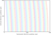 |
Fig. 13 Coordinate map of a subset of spectra on the detector (in pixels). The wavelength coordinate runs from blue (low) to red (high) for each selected MLA element. |
3.1.2 Fitting of the PSF
The parameters used to model the PSF are wavefront mode coefficients, that is: amplitudes of modes that when superposed describe the structure and amplitude of a phase screen. This screen represents the errors in the wavefront of the electric field in the pupil, which are produced by small scale manufacturing imperfections in the array of micro-optical systems that constitute the MLA, as well as in the optical elements that follow. In this paper, Zernike modes are used, that are considered generally the most suitable for modeling optical aberrations (Zernike 1934).
While the errors caused by imperfections in the main optical system are most likely rather uniform and simple, the imperfections between image elements in the MLA are predominantly uncorrelated, and may have any level of complexity. Generally, we thus have erratic variations, on top of a large scale, smoothly varying background.
The assumption is made here that the PSF is described by the same phase screen for all wavelengths. While there are good reasons to believe that this is an accurate assumption for the wavefront errors induced by the MLA, this is probably not the case for those introduced by the macroscopic spectrograph optics. The wavefront error may vary because the path taken through the optics is dependent on the spatial position of an MLA element, and the alignment error between the front and the back side lenses, but also by the wavelength of the light, which is varying along each spectrum.
Modeling the wavelength dependence
Although the wavelength dependence of the PSF is likely small, considering the spectral bandwidth of only 4.5Å, it cannot be excluded entirely either. Moreover, a smooth, large scale spatial variation of the PSF across the FOV would affect one side of the spectra differently from the other, and could thus be easily masquerade as a wavelength dependence.
Accommodating a wavelength dependent PSF has significant implications for the speed of the calculations, since the PSF must be separately calculated for each wavelength. However, as long as the quality of the fit is not perfect, and such wavelength dependence is probable, it is a price worth paying.
To differentiate between a spatially varying PSF masquerading as a chromatic aberration, we fit two models. The first one allowed explicitly for a smooth, large scale variation of the wave-front error across the FOV, which can vary along the spectral direction and manifest itself there as a pseudo chromatic variation. The variation itself was derived by fitting wavelength independent wavefront coefficients for each image element, but adding to that a wavefront error that is dependent on the position on the detector. This contribution was calculated by fitting a surface to each coefficient, from the fitted wavelength independent coefficients, as a function of the average position of the spectra. This procedure is repeated, and the global fit is updated, until convergence is reached. The fitted coefficients are thus reduced to wavefront corrections on top of a smooth background, and are expected to show no trend once convergence is reached. The second model explicitly allows a focus gradient along the spectral direction of each spectrum to be fitted, along with all the other wavefront coefficients, and assumes that this is the only source of wavelength dependent behavior.
While the first method visibly reduced the presence of moiré fringes in the residual, the averaged squared difference used as a metric for the optimization did not show a significant decrease compared to the wavelength independent optimization. The second method, that allows for an arbitrary focus gradient as a function of wavelength, however, reduced the moiré fringes even further, and additionally reduced the global metric by around 25%.
Figure 14 shows the value of the fitted focus gradient across the FOV. The smooth behavior suggests that this quantity is well constrained, and that it describes some large-scale properties of the instrument optics. Although, based on the reduction of the moiré fringes using a detector position dependent wavefront error, some of these properties must be purely position dependent, the improved behavior when allowing for an arbitrary focus gradient suggests that there is also a truly wavelength dependent component.
The map of the wavelength gradient unfortunately also shows an imprint of what is unmistakably the moiré pattern seen in Fig. 5. This is not expected, since the focus gradient is common to the whole spectrum of each image element, and should be influenced only by the average of the moiré pattern over many periods.
Based on the apparently superior results, the final optimization was carried out using a wavelength dependent focus gradient.
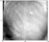 |
Fig. 14 Fitted wavelength gradient of the focus coefficient across the FOV. The gray scale runs from −4.8 × 10⁻³ to 5.6 × 10⁻³ waves per A. |
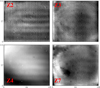 |
Fig. 15 Maps of the first 4 fitted Zernike mode coefficients for each image element. Z2(tip), Z3(tilt), Z4(focus) and Z7(astigmatism). |
Wavefront coefficients
As described above, the fitted coefficients contain all image element specific and all global optical aberrations, as far as they are not incorporated in the coordinate map. The spatial maps are therefore not expected to be very smooth, unless they are dominated by global optical imperfections. To arrive at a good fit, a selection of 25 modes between Noll indices 2 and 56 was required, where the order of the azimuthal components of the modes of higher radial order were kept low, thus introducing a preference for a relatively rotationally symmetric PSF.
Figure 15 shows the spatial distribution of the coefficients of the first 4 fitted modes. The first two, tip and tilt, describe the deviation of the spectral position relative to the coordinate values. Since the coordinate values are strongly regularized, these coefficients are expected to contain only the random position errors caused by front to back side microlens misalignments. If this is the main term influencing these coefficients, clearly, the misalignment is not purely randomly distributed. Nonlocal features are visible in the tip and tilt coefficients, consisting of vertical lines, with a periodicity of four image elements, and a slow, quasi-periodic oscillatory term, that appears to be closely aligned with the horizontal image coordinate.
The periodic vertical lines are all perfectly vertical, and thus are most likely associated with the MLA itself. This may be caused by a periodic error in the internal alignment between the front and the backside, or an interference between the MLA grid and the aperture mask on the back side, clipping or apodizing the pupil illumination. Although the underlying cause for this error remains unknown, since it is included in the map it should not affect the extracted data adversely. The cause of the periodic horizontal pattern is even less obvious, but may well be related to the detector.
The tilt coefficient map clearly contains an imprint of the moiré pattern, suggesting that the accuracy of the fit could still be improved somewhat.
Apart from the position and focus coefficients, the optimization shows a clear preference for Zernike mode 7, vertical coma, and its harmonics. The coefficient of this mode varies between −0.57 and 1.01 waves, which seems like a rather large range, but is probably the result of the pupil apodization shown in Fig. 7, caused by diffraction in the MLA. The effect of the apodization is to dampen the influence of the modes near the outer edge, which becomes increasingly significant with increasing radial order of the modes. The preference for a strong coma term is not immediately clear, but could be indicative of a less than optimal optical adjustment, especially of the secondary reimager.
This assessment is supported by the map of the focus coefficient that shows a variation from 0.21 to 0.64 waves across the FOV, with a clearly vertically oriented gradient. It also has a horizontal gradient in the amplitude, which gives it a fairly complex topology, which suggests that this is not the result of a simple alignment error, but a more complex performance issue, most likely of the secondary reimager.
With a satisfactory fit of the coefficients, the actual optical performance of the prototype can be calculated. To this end, we first obtain the PSF from the electric field distribution emerging from one MLA element, without any additional aberrations. Although the maximum value of this PSF represents the performance of a perfect instrument, and serves as the reference for the real PSFs, it already has a lower value than the diffraction limited PSF for an aperture of the dimensions of the spectrograph pupil, because the pupil illumination is apodized.
Figure 16 shows a map of the Strehl ratio, the maximum value of the PSF normalized with the reference value described above, at the center wavelength of the instrument, for each image element in the FOV. The mean of this map has a value of considerably less than one, and has a distribution that is roughly inversely proportional to that of the focus coefficient Z4 from Fig. 15. The maximum value of 0.73 is only 10% lower than the expected maximum of around 0.8 predicted by the optical model, but the lowest value is only 0.33, which is rather lower than expected, and another confirmation that the adjustment of the prototype may have been less than optimal.
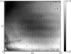 |
Fig. 16 Strehl ratio across the FOV of the MiHI prototype. |
Normalization of the transfer map
Although the integral of each map element of the transfer map over all image coordinates might be expected to yield a uniform value, because the PSF is not resolved by the detector pixels, and the detector has areas of reduced sensitivity, as described in Sect. 2.2.3, the transfer map fitted here does not meet that expectation. Instead, the total fraction of the incoming energy accounted for by the transfer map is always less than 1, where the exact value depends on the path of the spectrum across the areas of reduced sensitivity.
Therefore, it is important to ensure that the map elements are not clipped significantly, because this leads to a qualitative change in the transfer map. Especially, if the wings of the PSF are very wide, clipping the domain of the map elements leads to a transfer map with the same peak value, but the map element integrated over all space will be less than it should be. While this might not seem like such a big problem, it changes the amount of background signal, which in turn impacts the amplitude of the moiré fringes in the resulting image.
Figure 17 shows the modulation of the total integrated value of the transfer map elements, Mu,v,λ over all image coordinates (x, y), for a number of spatio-spectral slices from the transfer map. Although the fringe amplitude of nearly 3% clearly suggests that some light is lost as expected, presumably on the borders of the microlenses, it is much less than expected from the filling factor alone. This indicates that the PSF is not as compact as intended, and that most map elements extend over a significant number of pixel lines, thus averaging the modulation effect caused by the pixel borders.
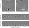 |
Fig. 17 Cuts through the integral over the transfer map. Top left: spatial cut at a wavelength coordinate of 200. Top right: spatial cut at a wavelength coordinate of 452. Middle: x − λ cut at y = 57. Bottom: y − λ cut at x = 63. The grayscale runs from 0.855 to 0.883 in all panels. |
3.2 Extracted data cube
Apart from the fitted coefficients that describe the parameterized model of the transfer map, the fit procedure returns as a byproduct the raw hyperspectral cube of the flat-field image. Far from being featureless, most of the nonuniformities in the transmission properties of the instrument, that are traditionally captured by a flat-field image, are still contained in it, as are the spectral features of the solar spectrum, as can be seen in Fig. 18. The figure shows 4 cuts through the data volume, two monochromatic slices at fixed wavelength, and two traditional spectra along the X and Y axes of the FOV respectively.
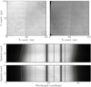 |
Fig. 18 Cuts through the extracted hyperspectral cube using the converged transfer map. Top left: spatial cut at a wavelength coordinate of 200. Top right: spatial cut at a wavelength coordinate of 452, Middle: x − λ cut at y = 57. Bottom: y − λ cut at x = 63. The yellow dashed lines highlight the filter boundaries, and show a significant drift of the prefilter passband across the FOV. |
3.2.1 Instrument transmission
Among the more prominent features in the spectra are the spectral lines, made to run perfectly vertical by the optimization of the coordinate map. The edges of the prefilter highlighted with yellow dashed lines, however, show a significant angle with respect to the vertical, indicating a drift in the spectral passband of the filter across the FOV. Especially in the X direction, the shift is seen to be close to half the separation between the two spectral lines, and thus must be around 500 mÅ, an unexpectedly large amount over an area of only 2×2 mm. It seems most likely that this drift is a filter property, and is not related to the angle of incidence of the beam, since the drift in the y direction is considerably less, but the beam properties are approximately symmetric.
The second significant feature is a marked difference in the brightness between the left and the right halves of the images. This division is also visible, but in a warped form, in the y − λ spectrum, running from the top left to the middle bottom of the spectrum. This difference in brightness cannot be associated with the transmission property of any particular optical component in the instrument, but is most likely a difference in the detector response between the left and right halves of the detector. This difference is also visible in low contrast images recorded with the camera, but is not visible in the raw data frames due to the intrinsically high contrast of the image.
The monochromatic slices in Fig. 18 clearly show a very regular pattern of vertical lines, that was determined to have a period of 4 MLA elements, and must originate in the MLA, since it aligns perfectly with the pixel grid, whereas any camera related defects are warped, as discussed above. The pattern appears to be closely related to a similar pattern in Fig. 15, and in particular of the tip and the tilt components. If the lines in the wavefront coefficients are indeed the result of a periodic alignment error, as speculated in Sect. 3.1.2, this would result in part of the light falling outside the grating area, resulting in the vertical lines of reduced transmission that is observed in Fig. 18.
It is also clear from the images that there is some vignetting near the camera focal plane, that is by extension wavelength dependent. At wavelength index 452, it is rather clearly visible as a fuzzy dark band on the upper left side of the image, and a much sharper clipped lower left corner. Already at wavelength index 200, it is much reduced in strength, but a third vignette is now visible in the lower right corner.
Apart from these large scale features, there are dark image elements randomly distributed throughout the FOV, visible in the monochromatic slices as dark “pixels”. Most of these are the result of a misalignment of the backside microlens with the front side microlens that is so large, that most of the light never reaches the grating. Figure 19 shows two neighboring sample spectra, one of which has a transmission of only 8.3%. Due to the low transmission, the contamination of that spectrum by its neighbors is very high, nonetheless, the extraction has managed to recover a spectrum that closely resembles the solar atlas spectrum, and removed nearly all of the imprint of the neighbors. Clearly, some of the light of the misaligned pixels actually still propagates through the instrument and reaches the detector, except for a handful of the very darkest image elements.
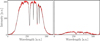 |
Fig. 19 Samples of two neighboring spectra (x, y) = (32, 26) (right) and (31, 26) (left) with a large difference in light transmission. Shown are the raw extracted data points (red) and the regularized spectra (black). |
3.2.2 Residuals
In Sect. 3.2, we discussed the raw data cubes, and its remaining imperfections. Because many of these imperfections are interfering with the optimization, the raw data were regularized, as described in Sect. 2.3.2 before use in the optimization. Because the difference between the raw and the regularized data contains information about the instrument that was filtered out of the optimization, we take a closer look at it here.
Figure 20 shows the relative difference between the raw and the regularized data cubes. Surprisingly, the division between the two camera halves, which is one of the strongest signals in the raw data, is not very prominent in the monochromatic slices of the residual. It is visible in the spectral slices, but only locally. This suggests that the difference itself was probably fitted and included in the transmission profile of the prefilter, and only the sharp transition between the two levels, that cannot be reproduced by the prefilter fitting procedure, remains.
The trajectory of the separation is still clearly visible in the spectral slice, and is accompanied by many other stripes that have the same general shape. Therefore, although they look like the residuals of moiré fringes, these are more likely to be gain differences between columns of the detector.
The monochromatic slices show a circular residual, that is visible at both the selected wavelengths, and is roughly centered on the FOV. It is large scale and smooth enough to be included in the model, and it stands out because it was not. This residual is clearly not an inaccurate fit to a strong feature, because the only feature resembling it in the raw data is actually difficult to make out. Indeed, several such rings can be seen with a position in the FOV that is a function of the wavelength, suggesting that the optimization failed to fit them simultaneously. No immediate root cause can be indicated for the appearance of these rings, and several other unconventional looking features, but their strength of 1–2% is compatible with the typical reflective losses on a broadband AR coated surface, of which there are many.
The remaining features in the residuals are clearly imperfections in the fitting of the moiré interference pattern, which appear to have an amplitude of 1–2%. This is a significant reduction compared to the fringes in the interpolated cubes from Sect. 2.1 with amplitudes of around 30%, but they are strong enough to remain visible. However, the parallel processing of the data and the flat-field images should ensure that most of this residual error is identical in the data and the flat-field, and thus cancels out, provided that the instrumental properties are sufficiently similar in both.
The residual is also a good place to spot problems or shortcomings in the optimization. The residual shown in Fig. 21 shows a partially converged result, and is a good example of this. At first sight this result appears to be rather well converged, but because the model does not include sufficiently high order wave-front terms, the spectral crosstalk is not corrected for. This causes two parasitic telluric lines to remain in the residual at a wavelength offset with respect to the actual telluric lines, the offset is indicated by the red and blue arrows.
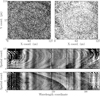 |
Fig. 20 Cuts through the hyperspectral cube of the relative residual. Top left: spatial cut at a wavelength coordinate of 200. Top right: spatial cut at a wavelength coordinate of 452. Middle: x − λ cut at y = 57. Bottom: y − λ cut at x = 63. The grayscale runs from −0.05 to 0.05 in all panels. |
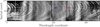 |
Fig. 21 x−λ cut through the hyperspectral cube of a partially converged relative residual, with inappropriate far wings. Clearly, the parasitic contamination of the blue telluric can be seen near the line centered on wavelength index 240, and to a lesser extent the one near the line centered on wavelength index 340. The solar lines leave only a very weak imprint, that is smooth enough to be partially included in the prefilter. |
 |
Fig. 22 Azimuthally averaged transfer functions for a perfect Strehl ratio of 1 (black), and two pixels with Strehl ratios of 0.63 (red) and 0.33 (blue) respectively. |
3.2.3 Spectral resolution
With the converged transfer map, we are now finally in a position to determine the spectral resolution of the instrument. We already established that there is a significant variability in the Strehl ratio over the FOV, which will have an impact on the S/N of the data. This does, however, not necessarily influence the spectral resolution of the instrument, it only affects the power with which the highest Fourier components in the spectral dimension (not to be confused with the highest frequencies in the spectral range) are transmitted.
When the transfer map is applied, the data are deconvolved, and the hyperspectral cubes should have a homogeneous spectral resolution, but with a variable S/N. Since we are undersampling the image plane, and selected the spectral grid to sample the image with a separation of approximately one spectral resolution element, we can only access spectral features that are at least twice as large as a detector pixel, and we therefore cannot measure the spectral resolution directly from the spectra.
We can, however, deduce it from the fitted PSFs, which are calculated with a grid spacing of 1/10th the size of a detector pixel, with the intention of significantly oversampling them, so that the PSF value can be assumed constant within each PSF pixel.
Figure 22 shows the transfer functions of a small sample of PSFs, co-plotted with a diffraction limited PSF. Clearly, the performance of the prototype is not optimal, but it is clear that some power is transmitted up to the diffraction limit of the spectrograph, at approximately 1.2 px−1, which, with a pixel size of approximately 10 mÅ, translates to 8.0 mÅ, or a spectral resolution of R = 756000.
Since we cannot expect to resolve frequencies below 0.5 px−1, indicated by the dotted line in the plot, we formally reach a resolution of only R = 315 000, and the spectral under-sampling even creates a potential for aliasing, the transformation of undersampled high frequencies to lower ones, in the spectral direction. The potential for this is dependent on the cutoff frequency of the data (see for instance Brault & White 1971), which depends on the S/N of the data and the signal content of the observed spectra.
4 Conclusions
We have modeled and characterized a MiHI prototype instrument for the purpose of data extraction and calibration. The high contrast of the raw hyperspectral data, the inability to recover the instrument gain in a simple way, and the small but significant variability of the instrument make this a necessary step to achieve the high quality data set required for scientific analysis.
The main task of the model that was developed here is the reproduction of the observed data, and in particular the moiré interference pattern in the data, that is intrinsic to the design of the instrument, and is highly sensitive to small changes of the image on the detector.
The model was able to accurately reproduce an average image of the Sun at disc center, under the assumption that the average solar spectrum is known, but only using an unexpectedly complex, wavelength dependent description for the PSF. The inability for the model to reproduce the observed data with a simple model suggests that the model is unique, and relates to the actual instrument properties.
The accurate reproduction of the observed image from a standard solar spectrum implies that the data that is extracted reliably represents the properties of the light present in the image plane of the telescope to a level of accuracy of 2–3%.
The sensitivity of the data to artifacts induced by instrumental changes is high, and is likely to be enhanced in any subsequent image restoration steps. Since this sensitivity is so high, the absence of strong instrumental artifacts in the data can be considered an indication that the characterization is accurate, and as a consequence that the data are well calibrated.
The characterization of the MiHI prototype is a critical step on the path to the general application of this type of integral field spectrograph for solar observations. The success of the present model in reproducing the observed flat-field data indicates that the required theoretical and numerical tools are sufficiently mature for use in the reduction of science data, which is the topic of the next paper in this series by Paper III.
Appendix A Program structure
The procedure that was used for the fitting of the parameters to the data is described briefly here, a diagram of the main structure of the computer code that was used for that is shown in Figure A.1. The steps in the flow diagram correspond approximately to the steps described in 2.2. Since the transfer map M is being fitted and is therefore changing between iterations, the data extraction using the symmetric least squares formalism from section 2.3.1 is not practical here, and the interpolation based method was used instead.
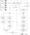 |
Fig. A.1 Program structure of the code used to determine the model fit parameters. |
Many of the steps are exceedingly time consuming, purely owing to the large number of image elements and fit parameters. With the selected data extraction algorithm, by far the largest amount of time is spent in the calculation of the map and its derivatives. This part of the calculation can be effectively parallelized, but the storage of the map and its derivatives requires a large amount of RAM. The execution of the code was therefore limited to 16 horizontal bands, with two rows of overlap between them, each of which exhausted all memory resources on our compute nodes. Since the spectral crosstalk is limited to only one row above and below, clipping one row on the top and bottom of each strip suffices to remove all edge effects.
Declaring the model converged was based predominantly on the value of the metric (the RMS difference between the input data frame and the synthesized image generated from the cleaned input hyperspectral cube), but also smoothness of the fit parameters and the residual were considered. Several optimization runs were carried out, with smoothing steps in between, bringing the coefficients closer to their expected values, without imposing external restrictions. Typically, the optimization finds a local minimum, in which no step can be found that further decreased the metric, after 10-100 iterations. The precise behavior depends strongly on the start conditions.
Appendix B Path integral
Here we present the expressions for the different segments of the path integral (2) used for the model of the MiHI prototype. We start by assuming that each PSF pixel of dimensions δ × δ is dispersed along a linear path segment. The pixel corner coordinates are given by:

and

The area A covered by the PSF pixel dispersed from t = tl to t = th generally has segments with no overlap, partial overlap, or full overlap with the detector pixel. The general expression is given by
 (B.1)
(B.1)
which we approximate here by assuming T(x, y) to be of binary form, as specified in (6). For full overlap of the PSF pixel with the active area of the detector pixel, this evaluates to
 (B.2)
(B.2)
For a limit on the lower boundary in the x direction only, we have

yielding
 (B.3)
(B.3)
Similarly, for a fixed upper limit in the x direction only, we have

yielding
 (B.4)
(B.4)
For a fixed upper and lower limit in the y direction only, we get
 (B.5)
(B.5)
and
 (B.6)
(B.6)
respectively.
For the cases where both dimensions are limited on the upper boundary, we get
 (B.7)
(B.7)
which has three more variations. For an upper limit in y and a lower limit in x we get
 (B.8)
(B.8)
for an lower limit in y and an upper limit in x we get
 (B.9)
(B.9)
and for an lower limit in y and x we get
 (B.10)
Assuming that the PSF pixels are smaller than the detector pixels, the final case of no overlap brings the total to 10 possibilities.
The evaluation of (B.1) now proceeds by determining the values of t for which the type of overlap with the current pixel changes from one type to another. The boundaries between path segments are set by the points on the path where the upper and lower limits of the PSF pixel under consideration in the x and y directions, x;, xh, yl, and yh respectively, coincide with the lower and upper detector pixel boundaries in the x and y directions, x−, x+, y− and y+ respectively, or by the wavelength limits for the specific wavelength bin λ− and λ+. The values of the path coordinate at the wavelength limits is arbitrary, and are conveniently set to 0 and 1 for the lower and upper wavelength limits respectively, the values for mx, my, cx, and cy are calculated to be consistent with that definition.
Since the type of overlap is changed by each limit of the PSF pixel crossing each limit of the detector pixel, there are potentially 8 limits where the type of overlap changes, and two imposed by the wavelength bin
 (B.11)
where the subscripts of t denote the reason for the limit (i.e.  marks the path coordinate for which the PSF pixel lower limit in x coincides with the detector pixel lower limit in x, etc.). These 10 coordinates bound a minimum of none, and a maximum of 9 separate line segments, any of which has a different type of overlap between the PSF and detector pixels.
We sort this list incrementally, after which we determine the type of overlap by calculating the center coordinate of each segment, and determining wether each of the four corners of the PSF pixel are contained in the area covered by the detector pixel, A. This procedure yields 4 binary values, with a total of 16 possible combinations, 6 of which can never occur: if 3 corners are contained in A, then the remaining corner must also be contained, and if two opposing corners are contained in A, the other two corners cannot be outside A. The 10 values that remain each correspond to one of the types of overlap described above. We can now exclude all path segments that do not result in overlap between the PSF and detector pixels, and calculate the sum over the contribution for all remaining segments.
Appendix C Derivatives
The derivatives of (B.2)..(B.10) are straightforward ifnot tedious to write down, but the dependencies must be considered carefully. We assume here that the offset of the path can change, but that the slopes of the path, mx and my, are constant. This is a good approximation if we assume that when the spectral path moves, on the scale of the full spectral range, the shape of the path does not change. The dependence of the integration limits tl and th on the coordinate offsets must be included though, so that although (B.2) does not have an apparent dependence on either cx or cy, the derivatives are potentially non-zero, because the area of overlap of the dispersed PSF pixel and the detector pixel can change. We thus have

and

With the spectral bin size chosen to be of the same order as the detector pixels, in most cases at least one of these will be nonzero, even if the PSF pixels are much smaller than the detector pixels.
For (B.3), we get

and

respectively, whereas (B.4) yields

and

Similarly, (B.5) has the derivatives

and

whereas (B.6) has the derivatives

and

The remaining four derivatives are considerably more complex, because of the coupled change in overlap on two sides, producing a second order dependence on t. (B.7) has the derivatives

and

(B.8) has the derivatives

and

(B.9) has the derivatives

and

and finally (B.10) has the derivatives

and

The expressions for  and
and  are readily calculated from(B.11)
 (C.1)
(C.1)
and are sorted to the same order as the path coordinates in appendix B. Although direct substitution of these expressions in the derivatives yields considerably simpler expressions, which derivative to select for substitution depends on the type of the neighboring segment, which is not known a priori. To keep the algorithm performing the calculations as generic as possible we leave the expressions as they are, and only substitute the values of the derivatives after sorting.
Acknowledgements
This research has made use of NASA’s Astrophysics Data System. This project was supported by the European Commission’s FP7 Capacities Programme under the Grant Agreements Nos. 212482 and 312495. It was also supported by the European Union s Horizon 2020 research and innovation programme under the Grant Agreements Nos. 653982 and 824135. The Swedish 1 m Solar Telescope is operated on the island of La Palma by the Institute for Solar Physics of Stockholm University in the Spanish Observatorio del Roque de los Muchachos of the Instituto de Astrofísica de Canarias.
References
- Allende Prieto, C., Asplund, M., & Fabiani Bendicho, P. 2004, A&A, 423, 1109 [NASA ADS] [CrossRef] [EDP Sciences] [Google Scholar]
- Antichi, J., Dohlen, K., Gratton, R. G., et al. 2009, ApJ, 695, 1042 [Google Scholar]
- Bacon, R., Adam, G., Baranne, A., et al. 1995, A&aS, 113, 347 [NASA ADS] [Google Scholar]
- Bacon, R., Emsellem, E., & Copin, Y. 2000, ASP Conf. Ser., 195, 173 [NASA ADS] [Google Scholar]
- Bacon, R., Copin, Y., Monnet, G., et al. 2001, MNRAS, 326, 23 [Google Scholar]
- Berdeu, A., Soulez, F., Denis, L., Langlois, M., & Thiébaut, É. 2020, A&A, 635, A90 [NASA ADS] [CrossRef] [EDP Sciences] [Google Scholar]
- Beuzit, J. L., Vigan, A., Mouillet, D., et al. 2019, A&A, 631, A155 [NASA ADS] [CrossRef] [EDP Sciences] [Google Scholar]
- Brandt, T. D., Rizzo, M., Groff, T., et al. 2017, J. Astron. Telesc. Instrum. Syst., 3, 048002 [CrossRef] [Google Scholar]
- Brault, J. W., & White, O. R. 1971, A&A, 13, 169 [NASA ADS] [Google Scholar]
- Chae, J., Park, H.-M., Ahn, K., et al. 2013, Sol. Phys., 288, 1 [NASA ADS] [CrossRef] [Google Scholar]
- de la Cruz Rodríguez, J., Löfdahl, M. G., Sütterlin, P., Hillberg, T., & Rouppe van der Voort, L. 2015, A&A, 573, A40 [NASA ADS] [CrossRef] [EDP Sciences] [Google Scholar]
- Delbouille, L., Roland, G., & Neven, L. 1973, Atlas photometrique du spectre solaire de [lambda] 3000 a [lambda] 10000 (Liège: Université de Liège) [Google Scholar]
- Dieter, Y., Daas, M., Dingfelder, J., et al. 2020, Nucl. Instrum. Methods Phys. Res. A, 972, 164130 [CrossRef] [Google Scholar]
- Doerr, H. P., Vitas, N., & Fabbian, D. 2016, A&A, 590, A118 [NASA ADS] [CrossRef] [EDP Sciences] [Google Scholar]
- El-Desouki, M., Jamal Deen, M., Fang, Q., et al. 2009, Sensors, 9, 430 [NASA ADS] [CrossRef] [Google Scholar]
- Fowler, B. 2006, in Proceedings of the ICIS ‘06 International Congress of Imaging Science (Society for Imaging Science and Technology) [Google Scholar]
- Groff, T. D., Kasdin, N. J., Limbach, M. A., et al. 2014, SPIE Conf. Ser., 9147, 91471W [NASA ADS] [Google Scholar]
- Henault, F., Bacon, R., Bonneville, C., et al. 2003, SPIE Proc., 4841, 1096 [NASA ADS] [CrossRef] [Google Scholar]
- Hinode Review Team, Al-Janabi, K., Antolin, P., et al. 2019, PASJ, 71, R1 [CrossRef] [Google Scholar]
- Horne, K. 1986, PASP, 98, 609 [Google Scholar]
- Kiselman, D., Pereira, T. M. D., Gustafsson, B., et al. 2011, A&A, 535, A14 [NASA ADS] [CrossRef] [EDP Sciences] [Google Scholar]
- Larkin, J., Barczys, M., Krabbe, A., et al. 2006, New A Rev., 50, 362 [CrossRef] [Google Scholar]
- Levenberg, K. 1944, Q. Appl. Math., 2, 164 [Google Scholar]
- Li, W., Ogunbona, P., Shi, Y., & Kharitonenko, I. 2002, in 2002 IEEE [Google Scholar]
- International Conference on Acoustics, Speech, and Signal Processing, 4, IV-3576 [Google Scholar]
- Livingston, W., Wallace, L., White, O. R., & Giampapa, M. S. 2007, ApJ, 657, 1137 [CrossRef] [Google Scholar]
- Löfdahl, M. G., & Scharmer, G. B. 1994, A&AS, 107, 243 [NASA ADS] [Google Scholar]
- Lohmann, A. W., Weigelt, G., & Wirnitzer, B. 1983, Appl. Opt., 22, 4028 [NASA ADS] [CrossRef] [Google Scholar]
- Macintosh, B., Graham, J., Palmer, D., et al. 2006, SPIE Conf. Ser., 6272, 62720L [Google Scholar]
- Marquardt, D. 1968, SIAM J. Appl. Math., 11, 431 [Google Scholar]
- Neckel, H. 1999, Sol. Phys., 184, 421 [Google Scholar]
- Northrop, R. B. 2014, Introduction to Instrumentation and Measurements (Boca Raton: CRC Press, Taylor & Francis Group), 3rd edn. [Google Scholar]
- Pavlov, A., Möller-Nilsson, O., Feldt, M., et al. 2008, SPIE Conf. Ser., 7019, 701939 [Google Scholar]
- Pereira, T. M. D., Kiselman, D., & Asplund, M. 2009, A&A, 507, 417 [NASA ADS] [CrossRef] [EDP Sciences] [Google Scholar]
- Robertson, J. G. 1986, PASP, 98, 1220 [Google Scholar]
- Rothenberg, T. J. 1984, Econometrica, 52, 811 [CrossRef] [Google Scholar]
- Scharmer, G. B., Bjelksjo, K., Korhonen, T. K., Lindberg, B., & Petterson, B. 2003, SPIE Conf. Ser., 4853, 341 [NASA ADS] [Google Scholar]
- Schnerr, R. S., de La Cruz Rodríguez, J., & van Noort, M. 2011, A&A, 534, A45 [NASA ADS] [CrossRef] [EDP Sciences] [Google Scholar]
- Tecza, M., Thatte, N. A., Eisenhauer, F., et al. 2000, SPIE Conf. Ser., 4008, 1344 [NASA ADS] [Google Scholar]
- van Noort, M. J., & Doerr, H.-P. 2022, A&A, 668, A151 [NASA ADS] [CrossRef] [EDP Sciences] [Google Scholar]
- van Noort, M. J., & Rouppe van der Voort, L. H. M. 2008, A&A, 489, 429 [NASA ADS] [CrossRef] [EDP Sciences] [Google Scholar]
- van Noort, M. J., Rouppe van der Voort, L., & Löfdahl, M. G. 2005, Sol. Phys., 228, 191 [NASA ADS] [CrossRef] [Google Scholar]
- van Noort, M. J., Kramer, A., Bischoff, J., Solanki, S. K. S., & Kiselman, D. 2022, A&A, 668, A149 [NASA ADS] [CrossRef] [EDP Sciences] [Google Scholar]
- von der Luehe, O. 1993, A&A, 268, 374 [Google Scholar]
- Webster, J. G. 1999, Measurement, Instrumentation, and Sensors Handbook (CRC Press) [Google Scholar]
- Zernike, V. F. 1934, Physica, 1, 689 [NASA ADS] [CrossRef] [Google Scholar]
All Figures
|
Fig. 1 Example of a darkfield corrected MiHI frame of a spatially featureless solar scene, obtained by averaging a large number of frames recorded at many different positions near the center of the solar disk. The image contains 5120 × 3840 pixels, the inset, highlighting the area in the red box, shows the individual spectra, packed onto the detector. The spectral direction runs from the upper left to the lower right, at an angle of approximately 3°, the boundaries of an example region containing a single spectrum are indicated by the yellow dashed lines. Spectral features belonging to adjacent image elements are separated horizontally. The image has two clearly visible brightness levels, the right half appearing systematically darker than the left one, a consequence of the uncorrected nonuniform gain of the camera. |
| In the text | |
|
Fig. 2 Example section of the ratio of a flat-field image, divided by another flat-field image recorded at a different solar elevation, for a 4 Å passband around 6302 Å. The blue dotted lines are the separation lines between the different rows of the MLA, the bright dots between the lines are produced by a pair of molecular O2 lines in this passband. |
| In the text | |
|
Fig. 3 2D histograms of the spectral feature density for one row of image elements for the spectral band at 589 nm (top) and the band at 656 nm (bottom). The grayscale indicates the point density as a function of normalized vertical coordinate (y axis), and horizontal position bin (x axis). Each dark band represents one or more telluric lines, with the bottom two bands of the top panel and the bottom band of the bottom panel containing two telluric lines each. |
| In the text | |
|
Fig. 4 Spectral features (black diamonds) produced on the detector by telluric lines in the spectral band between 5894 A and 5898 A, for one of the central rows of image elements. The solid red lines are fits to the high-density bands in Fig. 3, and accurately follow the positions of the spectral features on the detector. All spectral features located within a band around each red line (i.e. the area between the blue and green dashed lines) can be identified as resulting from a specific telluric line. Pairs of lines that cannot always be separated in the histograms (i.e. the lowest two bands in upper panel of Fig. 3) can now easily be separated and identified. |
| In the text | |
|
Fig. 5 Example of a raw MiHI data frame, recorded in the spectral region from 5891 to 5897 Å, containing a Ni line at 5892.7 Å, and the Na D1 line at 5895.9 Å, mapped to a 3D hyperspectral cube using the pixel association map only. The interpolation of the darkfield corrected raw image (left) to a series of monochromatic images (diagonal) also maps the moiré pattern, leading to a quasi-periodic fringe pattern in the monochromatic images. The spectrum, averaged over the FOV, shows clear signs of spectral crosstalk, manifesting as parasitic spectral lines, highlighted by the black arrows in the plot of the average spectrum (top right). The core intensity of the Na D1 line, that should be approximately 5% of the continuum intensity, is nearly 22%, suggesting that in this spectral band approximately 15% of the extracted intensity is coming from the neighboring spectra. |
| In the text | |
|
Fig. 6 Example of a path integral of the area of overlap of one PSF pixel. Left: overview of an area of 3 × 3 dector pixels, showing the area covered by a PSF pixel, dispersed over a spectral interval [t0 − t4] (red/green), and the detector pixel under consideration (gray). Right: detail showing the path, which is split up in four different segments. The types of overlap are: none (t0 − t1), top + left limited (t1 − t2), top limited (t2 − t3), and full overlap (t3 − t4). |
| In the text | |
|
Fig. 7 Electric field amplitude (left) and phase (right) in the output pupil of a single MLA element, on the compromised computational grid. The zeroed out area around the illuminated part of the pupil, needed to obtain an oversampled PSF is clipped. |
| In the text | |
|
Fig. 8 Response of a CMV20000 CMOS image sensor, averaged over the entire area (black), compared to a linear response (red-dotted line). |
| In the text | |
|
Fig. 9 Defect as a function of the iteration number for the interpolation based method (black) and the least squares fitting method (red). |
| In the text | |
|
Fig. 10 Difference of two data cubes, extracted from the same raw data frame with the interpolation based method and with the OLS based method, normalized by the mean continuum value of both cubes. Top left: spatial cut at a wavelength coordinate of 200. Top right: spatial cut at a wavelength coordinate of 452. Middle: x − λ cut at y = 57. Bottom: y − λ cut at x = 63. The grayscale runs from −0.01 to 0.01 in all panels. |
| In the text | |
|
Fig. 11 Difference of two spectra, extracted from the same raw data frame with the interpolation based method and with the OLS based method. Left: spectrum of the direct method (black) and the least squares method (red). Right: difference between the spectra from the left panel. |
| In the text | |
|
Fig. 12 Example of fitting the prefilter transmission curve. Left: raw extracted spectrum. Right: ratio of raw to reference spectrum (red) and the 10th order logarithmic fit (black). |
| In the text | |
|
Fig. 13 Coordinate map of a subset of spectra on the detector (in pixels). The wavelength coordinate runs from blue (low) to red (high) for each selected MLA element. |
| In the text | |
|
Fig. 14 Fitted wavelength gradient of the focus coefficient across the FOV. The gray scale runs from −4.8 × 10⁻³ to 5.6 × 10⁻³ waves per A. |
| In the text | |
|
Fig. 15 Maps of the first 4 fitted Zernike mode coefficients for each image element. Z2(tip), Z3(tilt), Z4(focus) and Z7(astigmatism). |
| In the text | |
|
Fig. 16 Strehl ratio across the FOV of the MiHI prototype. |
| In the text | |
|
Fig. 17 Cuts through the integral over the transfer map. Top left: spatial cut at a wavelength coordinate of 200. Top right: spatial cut at a wavelength coordinate of 452. Middle: x − λ cut at y = 57. Bottom: y − λ cut at x = 63. The grayscale runs from 0.855 to 0.883 in all panels. |
| In the text | |
|
Fig. 18 Cuts through the extracted hyperspectral cube using the converged transfer map. Top left: spatial cut at a wavelength coordinate of 200. Top right: spatial cut at a wavelength coordinate of 452, Middle: x − λ cut at y = 57. Bottom: y − λ cut at x = 63. The yellow dashed lines highlight the filter boundaries, and show a significant drift of the prefilter passband across the FOV. |
| In the text | |
|
Fig. 19 Samples of two neighboring spectra (x, y) = (32, 26) (right) and (31, 26) (left) with a large difference in light transmission. Shown are the raw extracted data points (red) and the regularized spectra (black). |
| In the text | |
|
Fig. 20 Cuts through the hyperspectral cube of the relative residual. Top left: spatial cut at a wavelength coordinate of 200. Top right: spatial cut at a wavelength coordinate of 452. Middle: x − λ cut at y = 57. Bottom: y − λ cut at x = 63. The grayscale runs from −0.05 to 0.05 in all panels. |
| In the text | |
|
Fig. 21 x−λ cut through the hyperspectral cube of a partially converged relative residual, with inappropriate far wings. Clearly, the parasitic contamination of the blue telluric can be seen near the line centered on wavelength index 240, and to a lesser extent the one near the line centered on wavelength index 340. The solar lines leave only a very weak imprint, that is smooth enough to be partially included in the prefilter. |
| In the text | |
|
Fig. 22 Azimuthally averaged transfer functions for a perfect Strehl ratio of 1 (black), and two pixels with Strehl ratios of 0.63 (red) and 0.33 (blue) respectively. |
| In the text | |
|
Fig. A.1 Program structure of the code used to determine the model fit parameters. |
| In the text | |
Current usage metrics show cumulative count of Article Views (full-text article views including HTML views, PDF and ePub downloads, according to the available data) and Abstracts Views on Vision4Press platform.
Data correspond to usage on the plateform after 2015. The current usage metrics is available 48-96 hours after online publication and is updated daily on week days.
Initial download of the metrics may take a while.