| Issue |
A&A
Volume 667, November 2022
|
|
|---|---|---|
| Article Number | A44 | |
| Number of page(s) | 10 | |
| Section | Stellar structure and evolution | |
| DOI | https://doi.org/10.1051/0004-6361/202244300 | |
| Published online | 04 November 2022 | |
The statistical properties of early-type stars from LAMOST DR8⋆
1
Yunnan Observatories, Chinese Academy of Sciences, PO Box 110, Kunming 650011, PR China
e-mail: This email address is being protected from spambots. You need JavaScript enabled to view it.
2
School of Astronomy and Space Science, University of Chinese Academy of Sciences, Beijing 100049, PR China
e-mail: This email address is being protected from spambots. You need JavaScript enabled to view it.
3
Key Laboratory for Structure and Evolution of Celestial Objects, Chinese Academy of Sciences, PO Box 110, Kunming 650216, PR China
4
Key Laboratory of Space Astronomy and Technology, National Astronomical Observatories, Chinese Academy of Sciences, Beijing 100101, PR China
5
Center for Astronomical Mega-Science, Chinese Academy of Sciences, 20A Datun Road, Chaoyang District, Beijing 100012, PR China
Received:
19
June
2022
Accepted:
18
July
2022
Abstract
Context. Massive binary stars play a crucial role in many astrophysical fields. Investigating the statistical properties of massive binary stars is essential to trace the formation of massive stars and constrain the evolution of stellar populations. However, no consensus has been achieved on the statistical properties of massive binary stars, mainly due to the lack of a large and homogeneous sample of spectroscopic observations.
Aims. We study the intrinsic binary fraction fbin and distributions of mass ratio f(q) and orbital period f(P) of early-type stars (comprised of O-, B-, and A-type stars) and investigate their dependences on effective temperature Teff, stellar metallicity [M/H], and the projection velocity vsini, based on the homogeneous spectroscopic sample from the Large Sky Area Multi-Object Fiber Spectroscopic Telescope (LAMOST) Data Release Eight (DR8).
Methods. We collected 886 early-type stars, each with more than six observations from the LAMOST DR8, and divided the sample into subgroups based on their derived effective temperature (Teff), metallicity ([M/H]), and projected rotational velocity (vsini). Radial velocity measurements were archived from a prior study. A set of Monte Carlo simulations, following distributions of f(P)∝Pπ and f(q)∝qγ were applied to the observed binary fraction to correct for any observational biases. The uncertainties of the derived results induced by the sample size and observation frequency are examined systematically.
Results. We found that fbin increases with increasing Teff. For stars in groups of B8-A, B4-B7, O-B3, the binary fractions are fbin = 48% ± 10%, 60%±10%, and 76%±10%, respectively. The binary fraction is positively correlated with metallicity for spectra in the sample, with derived values of fbin = 44% ± 10%, 60%±10%, and 72%±10% for spectra with metallicity ranges of [M/H] < −0.55, −0.55 ≤ [M/H] < −0.1, to [M/H] ≥ −0.1. Over all the vsini values we considered, the fbin have constant values of ∼50%. It seems that the binary population is relatively evenly distributed over a wide range of vsini values, while the whole sample shows that most of the stars are concentrated at low values of vsini (probably from strong wind and magnetic braking of single massive stars) and at high values of vsini (likely from the merging of binary stars). Stellar evolution and binary interaction may be partly responsible for this. In the case of samples with more than six observations, we derived π = −0.9 ± 0.35, −0.9 ± 0.35, and −0.9 ± 0.35, and γ = −1.9 ± 0.9, −1.1 ± 0.9, and −2 ± 0.9 for stars of types O-B3, B4-B7, and B8-A, respectively. There are no correlations found between π(γ) and Teff, nor for π(γ) and [M/H]. The uncertainties of the distribution decrease toward a larger sample size with higher observational cadence.
Key words: methods: data analysis / methods: statistical / surveys / stars: early-type
Full Table 2 is only available at the CDS via anonymous ftp to cdsarc.cds.unistra.fr (130.79.128.5) or via https://cdsarc.cds.unistra.fr/viz-bin/cat/J/A+A/667/A44
© Y. Guo et al. 2022
 Open Access article, published by EDP Sciences, under the terms of the Creative Commons Attribution License (https://creativecommons.org/licenses/by/4.0), which permits unrestricted use, distribution, and reproduction in any medium, provided the original work is properly cited.
This article is published in open access under the Subscribe-to-Open model. This email address is being protected from spambots. You need JavaScript enabled to view it. to support open access publication.
1. Introduction
Many studies show that most stars are in binary systems (Heintz 1969; Abt & Levy 1976; Duquennoy & Mayor 1991; Machida et al. 2008), especially early-type stars (Sana et al. 2012; Chini et al. 2012; Duchêne & Kraus 2013; Dunstall et al. 2015; Moe & Di Stefano 2017). Statistical analyses of binary stars, including intrinsic binary fractions, distributions of orbital period, and mass ratios, are important tracers of stellar formation and basic physical inputs for binary population synthesis (Sana et al. 2013; Liu 2019; Han et al. 2020). In particular, massive binaries and their statistical properties are essential for understanding compact objects’ formation. These include double black holes, double neutron stars, and neutron star–black hole binaries, as they are the dominant gravitational wave sources for the Laser Interferometer Gravitational-wave Observatory (LIGO), Virgo and KAGRA detectors (Abbott et al. 2016a,b; Chen et al. 2018; Han et al. 2020; Langer et al. 2020).
Among the statistical properties, the binary fraction fb is one of the most critical parameters, and it has been widely explored over the past few decades (Carney 1983; Henry & McCarthy 1990; Duquennoy & Mayor 1991; Fischer & Marcy 1992; Mason et al. 1998; Latham et al. 2002; Kratter et al. 2010; Rastegaev 2010; Raghavan et al. 2010; Duchêne & Kraus 2013; Sana et al. 2013; Tanaka & Omukai 2014; Moe & Di Stefano 2017; Liu 2019). These studies show that the binary fraction may depend on the mass, metallicity, and population age of the sample stars. The results from the various studies differ, and are controversial in some cases. For example, Sana et al. (2012) reported that Galactic O-type stars have an estimated binary fraction of 69%, while Kobulnicky et al. (2014) suggested a binary fraction of 51% for O-type stars using a different sample of stars. Latham et al. (2002) reported no correlation between the fb and metallicity for stars in their sample. Later works by Raghavan et al. (2010), Tian et al. (2018), and Liu (2019) suggest that an anti-correlation of the binary fraction and metallicity appears in their studies. Alternatively, a positive correlation between these two quantities was reported from Carney (1983) and Hettinger et al. (2015).
For the studies mentioned above, many works were based on small sample sizes, and on heterogeneous samples, especially for massive stars or early-type stars. The ongoing spectroscopic surveys, such as the Sloan Digital Sky Survey (SDSS; York et al. 2000) and the Large Sky Area Multi-Object Fiber Spectroscopic Telescope (LAMOST; Cui et al. 2012; Liu et al. 2020), provide good opportunities to study stellar statistical properties with huge homogeneous samples. Yuan et al. (2015) found an average binary fraction of 41%±2% for field FGK-type stars using spectroscopic sample from the SDSS. The fractions (at least 10%) of carbon-enhanced metal-poor (CEMP) stars and double-lined spectroscopic binaries, based on metal-poor stars selected from SDSS, are investigated by Aoki et al. (2015). Based on low-resolution observation from the LAMOST DR5, Luo et al. (2021) reported a binary fraction of 40% for O- and B-type stars in the sample using spectra with more than three observations. Later work by Guo et al. (2022) utilizing the medium-resolution spectra with a cadence of more than two from the LAMOST DR7 suggests a binary fraction of 68% for the early-type OB stars.
In the work of Guo et al. (2022, hereafter Paper I), the relative radial velocity is obtained by a maximum likelihood estimation, and a star is recognized as a binary according to the maximum variation of radial velocity. The intrinsic binary fraction can be obtained by correcting for any observational biases appearing in the sample using a series of Monte Carlo simulations from Sana et al. (2013). Since most of the early-type star spectra from Guo et al. (2022) only have two observations, significant errors would exist, although the large number of stars in the sample may reduce the errors to a certain degree. This influence has not been examined and corrected due to the small cadence number of spectra from LAMOST DR7. For the same reason, the dependence of the statistical properties on metallicity is not investigated in Paper I.
Motivated by the recent release of more than six million medium-resolution spectra from LAMOST DR8, in this paper we examine the uncertainties of the method used in Paper I and Sana et al. (2013), using both the sample size and the number of observations. We aim to improve the investigation of the binary fraction for early-type stars in the LAMOST DR8 database using an increased sample size (886 stars) with a higher observational cadence (≥6) to determine the dependences of the statistical properties of these stars on their metallicity.
The structure of the paper is as follows. We introduce the data of LAMOST-MRS in Sect. 2. In Sect. 3 we describe our work of dividing the sample into different groups based on their parameters and radial velocity (RV) measurements, and the criterion for identifying binaries. We briefly describe the Monte Carlo method used to correct the observational bias, the consistency check, and the details of testing the suitability of this method in Sect. 4. We report the results of the relationships between the statistical properties and the stellar spectral types, as well as the metallicity for early-type belonging to various subgroups from LAMOST DR8 in Sect. 5. The summary and our conclusions are presented in Sect. 6.
2. LAMOST data and sample
LAMOST is a four-meter quasi-meridian reflecting Schmidt telescope located at the Xinlong station of the National Astronomical Observatory, implemented with 4000 fibers. Both medium-resolution spectrographs with a resolving power of R ∼ 7500 and low-resolution spectrographs with a resolving power of R ∼ 1800 were installed on the telescope (Cui et al. 2012; Zhao et al. 2012; Deng et al. 2012). In October 2018, LAMOST began a new medium-resolution survey (MRS) to obtain multi-epoch observations. The spectra of MRS observations made from the blue arm have a wavelength range of 495 − 535 nm, and cover a wavelength range of 630 − 680 nm for the red arm (Liu et al. 2020).
Guo et al. (2021) utilized the spectra from the LAMOST MRS database to derive the atmospheric parameters of 9382 early-type stars via a data-driven technique called stellar label machine (SLAM; Zhang et al. 2020a,b). In this study, we adopt the early-type stars from Guo et al. (2021) to investigate their statistical properties.
3. Sample selection and RV measurements
3.1. Classifying the sample
As mentioned in Sect. 1, both the sample size and observation frequency affect the uncertainty of binary fraction and the distributions for mass ratio and orbital periods. In the work of Sana et al. (2013) about 93% of the samples have more than six observations. Luo et al. (2021) found that an increase in the observational frequency of a sample may lead to smaller uncertainties. We thus selected the sample with more than six observations from the catalog of Guo et al. (2021) for our study. There are a total of 886 stars in the sample. We also did some tests on the effect of observational frequencies and sample size to examine the uncertainties of the method, and the results are shown in Sect. 5.
Based on the atmospheric parameters given by Guo et al. (2021), we divided the samples into different groups according to three observables: effective temperature (Teff), metallicity ([M/H]), and projected rotational velocity (vsini). We simply divided the sample stars into low, medium, and high groups based upon their spectral types, metallicity, and vsini because the aim of the grouping is to explore trends between those atmospheric parameters and the binarity of the samples. For Teff, we divided the 886 samples into three groups (B8-A, B4-B7, O-B3)1 to investigate the relationships between Teff and statistical properties. We display the number distribution of stars classified by spectral types of B8-A (dotted blue line), B4-B7 (solid blue line), and O-B3 (dashed blue line) in the top panel of Fig. 1. The sample distribution from Sana et al. (2013) is denoted in solid purple. For [M/H], we divided the 886 stars into groups of [M/H] < −0.55 (red dashed line), −0.55 ≤ [M/H] < −0.1 (solid red line), [M/H] ≥ −0.1 (red dotted line), shown in the middle panel of Fig. 1. The black dashed line and the black dotted line represent the stars with vsini < 35 km s−1 and the stars with vsini larger than 70 km s−1, respectively, in the bottom panel of Fig. 1. The number distribution of stars with 35 ≤ vsini < 70 km s−1 is shown in the solid black line. The grouped sample sizes are displayed in Table 1.
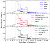 |
Fig. 1. Number distribution for different groups based on Teff (top panel), [M/H] (middle panel), and vsini (bottom panel). The solid purple line represents the observations of samples from Sana et al. (2013) in which about 93% of the sample are from more than six observations. |
Sample size of each group.
3.2. Radial velocity measurements
The data reduction was carried out via the standard LAMOST 2D pipeline, and the wavelength calibration was accomplished using the Sc and Th-Ar lamps for MRS spectra. The typical accuracy of wavelength calibration is 0.005 nm pixel−1 for LAMOST-MRS (Luo et al. 2015; Guo et al. 2022; Ren et al. 2021).
However, Liu et al. (2019) and Zhang et al. (2021) concluded that significant systematic errors exist among the RVs obtained from spectra collected by the different spectrographs, the exposures of LAMOST MRS surveys, and the temporal variations of the RV zero-points. Therefore, Zhang et al. (2021) applied a robust self-consistent method using Gaia DR2 RVs to determine the RV zero-points (RVZPs) from the exposures for each spectrograph of LAMOST after measuring the RVs based on the cross-correlation function method.
We cross-matched our 886 early-type stars with the updated RV catalog2 for LAMOST DR8 from Zhang et al. (2021) and adopted their corrected RV measurements. In Table 2, for each star we list the observation ID, coordinates, MJD date, S/N, Teff, [M/H], vsini, RV, and the uncertainty (σi).
Radial velocity catalogs.
3.3. Criterion for the binary
To identify the binaries in our sample, we adopted Eq. (4) from Sana et al. (2013), which states that a star is a binary if its RVs satisfy
 (1)
(1)
where vi(j) is the RV measured from the spectrum at epoch i(j) and σi(j) is the associated uncertainty. This criterion has been applied in several similar studies, for example Sana et al. (2012), Dunstall et al. (2015), Luo et al. (2021), Mahy et al. (2022), Banyard et al. (2022), and Guo et al. (2022).
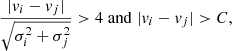
According to statistical standards, the confidence threshold of 3σ suggests a probability of finding 30 false detections in a sample of 1000 data entries, and this threshold is sufficient to filter out any outliers. We adopted a stricter criterion of 4σ, as suggested by Sana et al. (2013). This threshold criterion indicates a probability of finding one false detection in every 1000 entries.
The threshold C is used here to filter stars with pulsations, which may also lead to significant RV variation. Sana et al. (2013) adopted C = 20 km s−1 for O-type stars, and Dunstall et al. (2015) adopted C = 16 km s−1 for B-type stars, based on the kinks in the RV distributions of their sample. We did not find the appearance of a kink feature in our sample, hence simply adopted C = 16 km s−1 as that in Dunstall et al. (2015) because our sample is dominated by B-type stars.
The observed binary fraction  could be underestimated by the constraint of C because of the binary stars, even with large RV amplitudes, but small phase differences of the spectroscopic observations might be missed, and similarly binaries with relatively small RV variations might also be missed. Moreover, a large value of C would lead to a small value of
  from the same sample. However, this biases could be corrected by the Monte Carlo simulation described in Sect. 4. Here we just show (see Fig. 2) the results of the corrections for the O-B3 group. In the figure, the circles represent the observed binary fractions (
 ) of binaries in the sample (i.e., without applying any corrections), and these distributions are heavily affected by the arbitrary choice of C values. The squares stand for the intrinsic binary fractions (
 ) after correcting any observational biases using a Monte Carlo simulation (discussed in Sect. 4.1). As shown in the figure, the intrinsic binary fractions are constantly distributed over the C values, suggesting that it is safe to adopt the C = 16 km s−1 threshold criterion Mahy et al. (2022).
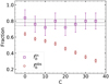 |
Fig. 2. Variations in the binary fraction of observation ( |


4. Correction for observational biases
4.1. Monte Carlo method
Here we use the approach described in Sana et al. (2013), where several Monte Carlo (MC) simulations are run to assess the intrinsic binary fraction ( ) based on
  . To perform the simulations, we need to construct two synthetic cumulative distributions (CDF) of RV variation (ΔRV), the peak-to-peak RV variation of each star, and the minimum timescale between the exposures (ΔMJD) by assuming the orbital configurations. We use a power law to describe the distribution for both the orbital period P and mass ratio q: f(P)∝Pπ and f(q)∝qγ. We do not use (log P) ∝ (log P)π, as is done in the literature, because the linear form is more sensitive to short-period binaries (Guo et al. 2022). Table 3 lists the variable ranges for the above parameters and power index. We adopt the initial mass function (IMF) from Salpeter (1955) with α = −2.353 for the primary masses (Mahy et al. 2022).
Range of different parameters and power indexes used in MC simulation.
In general, two-body kinetic systems in a Keplerian orbit are described by the orbital parameters, which are inclination (i), semimajor axis (a), the argument of periastron (ω), eccentricity (e), and the epoch of periastron (τ). The inclination is randomly drawn over an interval from 0 to π/2 and satisfies a probability distribution of sin(i). The semimajor axis is correlated to the orbital period (P). The ω satisfies a uniform distribution randomly drawn from it from 0 to 2π. We use eη to describe the distribution in which η is set to −0.5 from Sana et al. (2013), and τ is selected randomly in units of days.
With the above assumptions we can obtain the simulated RV to further simulate the CDF distribution of ΔRV and ΔMJD. The example for the simulated CDF of ΔRV and ΔMJD is shown in Fig. 3. The constructed simulated CDFs are compared with the observed ones by using Kolmogorov–Smirnov (KS) test, and the simulated and observed fractions of detected binaries ( and
and  ) are compared using binomial distribution (Sana et al. 2013). We then use the optimum values from the global merit function (GMF) projection, following Sana et al. (2013), to estimate the final results. The GMF consists of the KS probabilities of ΔRV and ΔMJD distributions and the binomial probability
 (2)
(2)
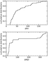 |
Fig. 3. Example of the simulated CDF of ΔRV and ΔMJD with the input parameters of |

where Nb is the number of binaries in the observations, while N is the sample size.
To examine the applicability of the GMF for stars (more than six observations) from the LAMOST-MRS, we constructed 24 600 synthetic CDFs with the known input sets of  , π, and γ. Figure 4 shows the choices of the known input sets of the parameters. We then compare the input parameters with the simulated parameters and show the projections of residuals for the comparisons in Fig. 5. The residuals are the differences between the output parameters predicted by the simulations and the input known parameters. The projection is the distribution of the residuals in which the histogram is the marginal distribution for each parameter. For each parameter, we use the 50th percentile of marginal distribution from the residual distributions to estimate offset and mean values of the 16th percentile (p16) and the 84th percentile (p84) to estimate errors. We estimated the uncertainty (unc) using the offset and error of each parameter through error propagation: unc =
  . The final uncertainties are
  , π = 0.35, and γ = 0.9. We see in the figure that the intrinsic properties (input) are well reproduced by the Monte Carlo simulation without systematic bias (p50 = 0), which verifies the reliability of our method.
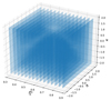 |
Fig. 4. Choices of input sets of |


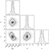 |
Fig. 5. Projections of residuals from the comparisons of input known parameters and output parameters. |
We also reanalyzed the 360 O-type stars in the sample of Sana et al. (2013). We obtained statistical properties of the sample consistent with those of Sana et al. (2013; see Paper I for details).
4.2. Impact of observational frequency and sample size
In order to investigate the effect of observational frequencies and the sample sizes on the final results, we performed the three sets of tests.
First, we examined the impact of observation frequency by using the same sample of stars (N = 154, the same sample size as O-B3), but with different observational frequencies n (i.e., n = 2, 3, 4, 5 and 6). The result is shown in the left panel of Fig. 6, where the black open and filled squares (plus signs) represent the error and offset (uncertainties). More detailed calculations are described in Sect. 4.1. We see that the uncertainty of each parameter becomes smaller with increasing observational frequency, as expected (Luo et al. 2021). In particular, the offset for all three parameters becomes zero when n = 6.
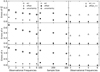 |
Fig. 6. Uncertainties for the different samples. Left panel: open and filled squares represent the error and offset of the same sample of stars, but with different observational frequencies. The plus signs represent uncertainties. Middle panel: open and filled circles represent the error and offset of the same observational frequencies sample of stars, but with different sample sizes. The plus signs represent uncertainties. Right panel: open and filled triangles represent the error and offset of the actual samples. The uncertainties are not shown because they have the same values as the errors. |
We then investigated the effect of the sample size. We used three samples with the number of stars N = 100, 200, and 300, and the observational frequency n set to 5 (the result of n = 6 is similar to n = 5; here we take 5 as an example). The middle panel of Fig. 6 shows the results. It indicates that the uncertainty decreases with the increasing number of stars, especially for π and γ.
We find that both big sample size and a high observational frequency would reduce the uncertainty of the method. However, for the real data the sample size generally decreases with increasing observational frequency. We therefore make the uncertainty estimates using the number of observations and the sample size of the real sample. We consider four samples here, with n ≥ 3, 4, 5, and 6. The number of stars in each sample is N = 459, 300, 240, and 154. The results are shown in right panel of Fig. 6. We see that the uncertainties of binary fraction  are very similar (around 0.1) for all the cases, while the uncertainties of π and γ are slightly smaller for the cases of n ≥ 3, 4 than that for the cases of n ≥ 5, 6. The sample size could be the cause for this. This test indicates that the number of stars in the sample may indeed reduce the uncertainty of the results induced by the observational frequency. In the following, we show all the results from the samples with observational frequencies greater than 3, 4, 5, and 6, and selected the case of n ≥ 6 as the standard to compare with previous studies.
5. Results and discussions
Figures 7–9 show the intrinsic statistical properties of  , π, and γ for various samples, with observation frequency n ≥ 3, 4, 5, and 6, and the dependences of these parameters on the spectral type, metallicity, and projection velocity vsini.
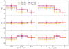 |
Fig. 7. Intrinsic statistical properties of |


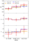 |
Fig. 8. Intrinsic statistical properties of |

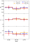 |
Fig. 9. Intrinsic statistical properties of |

5.1. Dependence on Teff
Figure 7 shows the dependence of  , π, and γ on the spectral type. We note that the intrinsic binary fraction
  is positively correlated with Teff (i.e., the intrinsic binary fractions increased toward the early-type stars), which is consistent with the result of Raghavan et al. (2010), Duchêne & Kraus (2013), Moe & Di Stefano (2017), and Guo et al. (2022). Marks & Kroupa (2011) also argued that binaries born preferentially efficiently with larger primary mass (Liu 2019).
For the cases of n ≥ 5 and 6, the binary fraction is 76%±10%, 60%±10%, and 48%±10% for stars of O-B3, B4-B7, and B8-A types, respectively. The binary fraction for stars of types B4-B7 and B8-A in the cases of n ≥ 3 and 4 becomes smaller (fb = 48%±10%) which is expected. For a large observation frequency (i.e., n ≥ 5 or 6), there is a high possibility of obtaining the maximum RV difference of a binary, resulting in more binaries to be verified in comparison to the cases of relatively low observation frequencies. The results for n ≥ 5 and 6 are very similar, indicating that 5 and 6 times are the optimal numbers of the observational frequencies for this method.
Figure 10 shows the  for the sample of n ≥ 6 in comparison to that in the literature. We see that the result of O-B3-type stars in our study agrees well with that of Galactic O-type stars (
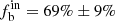 , filled squares) from Sana et al. (2012), and that
  in our sample is significantly higher than that given by Luo et al. (2021) for the OB stars from LAMOST DR5 (about 40%, with filled circles). In the study of Luo et al. (2021), most of stars (80%) in the sample have three observations. As seen in Fig. 7, the binary fraction is about 48% for B4-A stars for the sample of n ≥ 3, which is consistent with the result of Luo et al. (2021) within the uncertainties. The binary fraction in Guo et al. (2022) is systematically lower than that of this study for each spectral type since most of the samples in Guo et al. (2022) have only two observations, leading to many binaries being missed by the method, as mentioned in Sect. 4.
 |
Fig. 10. Intrinsic statistical properties of |

The values of π and γ remain almost constant with the spectral type of stars, possibly indicating the same origins of the binary star formation with various temperatures in this range. Our study gives π = −0.9 ± 0.35, −0.9 ± 0.35, and −0.9 ± 0.35, and γ = −1.9 ± 0.9, −1.1 ± 0.9, and −2 ± 0.9 for stars of O-B3, B4-B7, and B8-A type, respectively.
5.2. Dependence on [M/H]
Figure 8 shows the results for different metallicities. It is clearly shown that the binary fraction  (the upper panel) increases with [M/H]. For the sample of n ≥ 6, with the highest
  obtained, the intrinsic binary fraction
  is 44%±10%, 60%±10%, and 72%±10% for [M/H] < −0.55, −0.55 ≤ [M/H] < −0.1, and [M/H] ≥ −0.1, respectively. The correlation between
  and [M/H] is still an open question and could be affected by several factors, such as star formation, binary evolution, or dynamical interaction of clusters, or any combination of the three (Hettinger et al. 2015). Machida et al. (2009) suggested that a metal-poor cluster is more likely to form binaries via cloud fragmentation, and this may explain some observations with high
  for metal-poor stars. However, Korntreff et al. (2012) argued that many short-period systems would merge shortly after formation since the density of gas for a newly formed cluster increases due to dynamical evolution of the cluster. Blue stragglers, formed by binary evolution or dynamical interaction of clusters, provide evidence for these processes (Yanny et al. 2000; Latham et al. 2002; Lu et al. 2010).
Similarly, we do not find obvious trends for the π and γ values with metallicity [M/H]. For [M/H] < −0.55, −0.55 ≤ [M/H] < −0.1, and [M/H] ≥ −0.1 we have π = −0.9 ± 0.35, −1.1 ± 0.35, and −0.7 ± 0.35, respectively, and γ = −3.5 ± 0.9, −3.1 ± 0.9, and −2.2 ± 0.9, respectively.
5.3. Dependence on the projection velocity of v sin i
The results for the dependence of statistical properties on the projection velocity are shown in Fig. 9. There is no evidence showing the correlation between the statistical parameters and vsini. The intrinsic binary fraction  is around 50% for all cases, as shown in the figure. For the sample of n ≥ 6, fb = 56%±10%, 48%±10%, and 48%±10%; π = −0.9 ± 0.35, −0.7 ± 0.35, and −0.9 ± 0.35; γ = −3.3 ± 0.9, −3.6 ± 0.9, and −3.9 ± 0.9 for vsini < 35 km s−1, 35 ≤ vsini < 70 km s−1, and vsini ≥ 70 km s−1, respectively.
The absorption lines of fast rotators (vsini over 200 km s−1) become very flat in medium-resolution spectra, which can only be detected by high-resolution spectra. These objects were therefore filtered out when we selected early-type stars based on equivalent widths of H and HeI lines (Guo et al. 2022). The number of the fast rotators is very small and does not have a significant impact on the results. On the other hand, the flat absorption lines would cause large RV errors, leading to an overestimate of  (since Eq. (1) could be satisfied more easily). In any case, the stars in groups of vsini < 70 km s−1 are not affected. For stars with vsini > 70 km s−1, we display the ΔRV distribution in Fig. 11 in comparison with the other two groups. We found that the three distributions are similar, indicating that the measurement of vsini in our sample is not significantly affected by the RV measurement. So the dependence of
  on vsini would not change due to these errors.
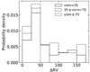 |
Fig. 11. Distribution of ΔRV in groups of vsini < 35 km s−1 (solid line), 35 ≤ vsini < 70 km s−1 (dashed line), and the stars with vsini larger than 70 km s−1 (dot-dashed line). |
Although the values of vsini estimated by the machine learning are systematically lower than those derived from high-resolution spectra (see Fig. 8 of Guo et al. 2021), the result that  has no correlation with vsini does not change. This is consistent with previous studies; for example, Fig. 1 at the website4 (Głȩbocki & Gnaciński 2005) shows that O, B, and A stars rotate faster than the stars later than A, while there is no obvious dependence between spectral type and vsini among O, B, and A stars. Our study is for O, B, and A stars, and is in close agreement.
Since the value of vsini may give hints to star formation and binary evolution, we further compare the frequencies of binary population and the whole sample on the value of vsini. Figure 12 shows the results based on the spectral type of the stars and Fig. 13 based on [M/H]. In both figures, the upper panel shows the distribution of vsini of the sample and the bottom panel is for the cumulative distribution (CDF). We see obvious differences in the CDFs between the binary populations and the whole samples.
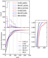 |
Fig. 12. Comparison of the vsini histograms (top panel) and cumulative distributions (bottom panel) based on different groups of Teff. The solid and dashed lines represent all the stars and binary samples, respectively. The red, blue, and black lines represent the samples in O-B3, B4-B7, and B8-A groups, respectively. |
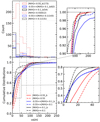 |
Fig. 13. Comparison of the vsini histograms (top panel) and cumulative distributions (bottom panel) based on different groups of [M/H]. The solid and dashed lines represent all the stars and binary samples, respectively. The red, blue, and black lines represent the samples in [M/H] < −0.55, −0.55 ≤ [M/H] < −0.1, and [M/H] ≥ −0.1 groups, respectively. |
In Fig. 12, for stars of O-B3 type (in red), the CDF of the whole sample, in comparison to that of the binary population, is larger when vsini < 40 km s−1 and gradually becomes smaller after that. This variation indicates that the likely single stars in the sample have a low-vsini group and a high-vsini group, while the binaries have a relatively flat distribution of vsini. This is possibly related to stellar evolution and binary interaction. The low-vsini group of the likely single stars is the result of strong wind and magnetic braking of massive single stars (Matt & Pudritz 2005; Ekström et al. 2008, 2012), while the high-vsini group is likely from the merger of binary stars (de Mink et al. 2013). Binary interaction gives the binary population a relatively wide range of vsini (or orbital periods if tidally locked). The case of stars with of types B4-B7 (in blue) is similar, but the high-vsini group of the likely single stars seems to have a relatively low vsini value (in the range of 50−100 km s−1) in comparison to that of O-B3 stars. It is a little different for B8-A-type stars (in black). The CDF of the binary population is larger than that of the whole sample when vsini < 100 km s−1, and becomes smaller after that. The CDF of the binary population also indicates a relatively wide range of binaries. In particular, there are some binaries having vsini slightly higher (vsini > 95 km s−1) than that of likely single stars.
The differences of the CDFs for various metallicity groups are more obvious than those grouped by spectral type. For those with high [M/H], most stars in the whole sample have low vsini, while the binary population span on a wide range of vsini. For those with intermediate [M/H], the CDFs of the whole sample and the binary population are very close when vsini < 40 km s−1. About 70% of both samples have vsini less than 40 km s−1. After vsini > ∼40 km s−1, the CDF of the whole sample increases faster than that of the binary population and is close to 1.0 when vsini = ∼240 km s−1, indicating the majority of the remaining 30% of the stars have vsini in 40−240 km s−1 in the whole sample. Similarly, the CDFs of the binary population span a very wide range of vsini values. About 1.5% of the binaries have vsini that can be larger than 250 km s−1, as shown by the CDF. We also see that a small part of the binary population have higher values of vsini in comparison to that of the whole sample for the case of low [M/H].
Several factors affect the values of vsini, from the fragmentation of clouds and the stellar wind of massive stars to the binary or dynamical interaction. It is hard to assess all the effects in quantity presently, and it is beyond the scope of this manuscript. It is clear to us, as shown in Figs. 12 and 13, that the binary population is quite evenly distributed over a wide range of vsini values. This property probably comes from binary evolution or interaction (i.e., the components of a binary are tidally locked with the orbit).
6. Conclusion
We collected 886 early-type stars with more than six observations from LAMOST DR8, divided the sample in three ways based upon effective temperature, metallicity [M/H], and projection velocity vsini, and investigated the statistical properties of the samples.
We first used the variations of radial velocities of each sample to identify the binaries in the sample and to obtain the observed binary fraction. Based on the Monte Carlo simulations in statistics, we corrected observational biases and estimated the intrinsic statistical properties of the binary fraction, the distributions of orbital period, and the mass ratio.
Our study shows that the intrinsic binary fraction increases with increasing Teff, consistent with what is found in the literature. We also find that the binary fraction is positively correlated with metallicity in our sample, consistent with Carney (1983) and Hettinger et al. (2015), but opposite to what is found in Tian et al. (2018) and Liu (2019). We do not find correlations between binary fraction and projection velocity vsini. However, it seems that the binary population is relatively evenly distributed over a wide range of vsini values, while the whole sample shows that most of the stars are concentrated at low values of vsini, and at high values of vsini in some cases. Binary evolution may partly account for this.
We examined the uncertainties in our method induced by the sample size and observation frequency systematically in the paper and found that the uncertainties of the statistical properties decrease with increasing sample size and the observation frequency. For the real sample of the LAMOST DR8, the uncertainty of  is similar (around 0.1) to that of the samples with observation frequency n ≥ 3, 4, 5, and 6. For the cases of n ≥ 5 and 6, we obtain the binary fraction of 76%±10%, 60%±10%, and 48%±10% for stars of O-B3, B4-B7, and B8-A type, respectively. The binary fraction becomes smaller (
 ) for the samples of n ≥ 3 and 4 since it has a low possibility to obtain the maximum RV difference of a binary, resulting in fewer binaries to be verified in these cases, in comparison to that of relatively high observation frequencies.
We do not find obvious correlations between the orbital period distribution f(P) (or the mass ratio distribution f(q)) and effective temperature Teff, and between f(P) (or f(q)) and metallicity [M/H], likely due to the short observational cadence. For the sample with n ≥ 6, we have π = −0.9 ± 0.35, −0.9 ± 0.35, and −0.9 ± 0.35, and γ = −1.9 ± 0.9, −1.1 ± 0.9, and −2 ± 0.9 respectively for stars of O-B3, B4-B7, and B8-A types.
We followed the same boundaries as used in Guo et al. (2022) to facilitate comparison with the previous results. There are four groups according to equivalent widths of He I and Hα: T1 (∼O-B4), T2 (∼B5), T3 (∼B7), and T4 (∼B8-A). We had not obtained effective temperature at that time. However, we found that the number in the first three groups (T1–T3, with six observations) is not large enough for the study. We therefore combined the first three groups and divided them into two groups, with B3–B4 as the boundary to ensure the two groups have similar samples.
We did a test with the IMF of Kroupa (2001) (i.e., alpha = −2.3 for M ≥ 1 M⊙) and obtained binary fractions similar to those shown in the paper.
Acknowledgments
This work is supported by the Natural Science Foundation of China (Nos. 2021YFA1600403/1, 12125303, 11733008, 12090040/3, 12103085) and by the China Manned Space Project of No. CMS-CSST-2021-A10. C.L. acknowledges National Key R\AMP D Program of China No. 2019YFA0405500 and the NSFC with grant No. 11835057. Guoshoujing Telescope (the Large Sky Area Multi-Object Fiber Spectroscopic Telescope LAMOST) is a National Major Scientific Project built by the Chinese Academy of Sciences. Funding for the project has been provided by the National Development and Reform Commission. LAMOST is operated and managed by the National Astronomical Observatories, Chinese Academy of Sciences. This work is also supported by the Key Research Program of Frontier Sciences, CAS, Grant No. QYZDY-SSW-SLH007.
References
- Abbott, B. P., Abbott, R., Abbott, T. D., et al. 2016a, Phys. Rev. Lett., 116, 061102 [Google Scholar]
- Abbott, B. P., Abbott, R., Abbott, T. D., et al. 2016b, Phys. Rev. Lett., 116, 241103 [Google Scholar]
- Abt, H. A., & Levy, S. G. 1976, ApJS, 30, 273 [Google Scholar]
- Aoki, W., Suda, T., Beers, T. C., & Honda, S. 2015, AJ, 149, 39 [NASA ADS] [CrossRef] [Google Scholar]
- Banyard, G., Sana, H., Mahy, L., et al. 2022, A&A, 658, A69 [NASA ADS] [CrossRef] [EDP Sciences] [Google Scholar]
- Carney, B. W. 1983, AJ, 88, 623 [NASA ADS] [CrossRef] [Google Scholar]
- Chen, X., Li, Y., & Han, Z. 2018, Sci. Sin. Phys. Mech. Astron., 48, 079803 [NASA ADS] [CrossRef] [Google Scholar]
- Chini, R., Hoffmeister, V. H., Nasseri, A., Stahl, O., & Zinnecker, H. 2012, MNRAS, 424, 1925 [Google Scholar]
- Cui, X.-Q., Zhao, Y.-H., Chu, Y.-Q., et al. 2012, Res. Astron. Astrophys., 12, 1197 [Google Scholar]
- de Mink, S. E., Langer, N., Izzard, R. G., Sana, H., & de Koter, A. 2013, ApJ, 764, 166 [Google Scholar]
- Deng, L.-C., Newberg, H. J., Liu, C., et al. 2012, Res. Astron. Astrophys., 12, 735 [Google Scholar]
- Duchêne, G., & Kraus, A. 2013, ARA&A, 51, 269 [Google Scholar]
- Dunstall, P. R., Dufton, P. L., Sana, H., et al. 2015, A&A, 580, A93 [NASA ADS] [CrossRef] [EDP Sciences] [Google Scholar]
- Duquennoy, A., & Mayor, M. 1991, A&A, 248, 485 [NASA ADS] [Google Scholar]
- Ekström, S., Meynet, G., Maeder, A., & Barblan, F. 2008, A&A, 478, 467 [Google Scholar]
- Ekström, S., Georgy, C., Eggenberger, P., et al. 2012, A&A, 537, A146 [Google Scholar]
- Fischer, D. A., & Marcy, G. W. 1992, ApJ, 396, 178 [NASA ADS] [CrossRef] [Google Scholar]
- Głȩbocki, R., & Gnaciński, P. 2005, in 13th Cambridge Workshop on Cool Stars, Stellar Systems and the Sun, eds. F. Favata, G. A. J. Hussain, & B. Battrick, ESA Spec. Publ., 560, 571 [Google Scholar]
- Guo, Y., Zhang, B., Liu, C., et al. 2021, ApJS, 257, 54 [NASA ADS] [CrossRef] [Google Scholar]
- Guo, Y., Li, J., Xiong, J., et al. 2022, Res. Astron. Astrophys., 22, 025009 [CrossRef] [Google Scholar]
- Han, Z.-W., Ge, H.-W., Chen, X.-F., & Chen, H.-L. 2020, Res. Astron. Astrophys., 20, 161 [CrossRef] [Google Scholar]
- Heintz, W. D. 1969, AJ, 74, 768 [NASA ADS] [CrossRef] [Google Scholar]
- Henry, T. J., & McCarthy, D. W., Jr. 1990, ApJ, 350, 334 [NASA ADS] [CrossRef] [Google Scholar]
- Hettinger, T., Badenes, C., Strader, J., Bickerton, S. J., & Beers, T. C. 2015, ApJ, 806, L2 [NASA ADS] [CrossRef] [Google Scholar]
- Kobulnicky, H. A., Kiminki, D. C., Lundquist, M. J., et al. 2014, ApJS, 213, 34 [Google Scholar]
- Korntreff, C., Kaczmarek, T., & Pfalzner, S. 2012, A&A, 543, A126 [NASA ADS] [CrossRef] [EDP Sciences] [Google Scholar]
- Kratter, K. M., Matzner, C. D., Krumholz, M. R., & Klein, R. I. 2010, ApJ, 708, 1585 [NASA ADS] [CrossRef] [Google Scholar]
- Kroupa, P. 2001, MNRAS, 322, 231 [NASA ADS] [CrossRef] [Google Scholar]
- Langer, N., Schürmann, C., Stoll, K., et al. 2020, A&A, 638, A39 [NASA ADS] [CrossRef] [EDP Sciences] [Google Scholar]
- Latham, D. W., Stefanik, R. P., Torres, G., et al. 2002, AJ, 124, 1144 [NASA ADS] [CrossRef] [Google Scholar]
- Liu, C. 2019, MNRAS, 490, 550 [NASA ADS] [Google Scholar]
- Liu, N., Fu, J.-N., Zong, W., et al. 2019, Res. Astron. Astrophys., 19, 075 [CrossRef] [Google Scholar]
- Liu, C., Fu, J., Shi, J., et al. 2020, Res. Astron. Astrophys., submitted [arXiv:2005.07210] [Google Scholar]
- Lu, P., Deng, L. C., & Zhang, X. B. 2010, MNRAS, 409, 1013 [NASA ADS] [CrossRef] [Google Scholar]
- Luo, A. L., Zhao, Y.-H., Zhao, G., et al. 2015, Res. Astron. Astrophys., 15, 1095 [Google Scholar]
- Luo, F., Zhao, Y.-H., Li, J., Guo, Y.-J., & Liu, C. 2021, Res. Astron. Astrophys., 21, 272 [Google Scholar]
- Machida, M. N., Tomisaka, K., Matsumoto, T., & Inutsuka, S.-I. 2008, ApJ, 677, 327 [CrossRef] [Google Scholar]
- Machida, M. N., Omukai, K., Matsumoto, T., & Inutsuka, S.-I. 2009, MNRAS, 399, 1255 [NASA ADS] [CrossRef] [Google Scholar]
- Mahy, L., Lanthermann, C., Hutsemékers, D., et al. 2022, A&A, 657, A4 [NASA ADS] [CrossRef] [EDP Sciences] [Google Scholar]
- Marks, M., & Kroupa, P. 2011, MNRAS, 417, 1702 [NASA ADS] [CrossRef] [Google Scholar]
- Mason, B. D., Henry, T. J., Hartkopf, W. I., ten Brummelaar, T., & Soderblom, D. R. 1998, AJ, 116, 2975 [NASA ADS] [CrossRef] [Google Scholar]
- Matt, S., & Pudritz, R. E. 2005, ApJ, 632, L135 [Google Scholar]
- Moe, M., & Di Stefano, R. 2017, ApJS, 230, 15 [Google Scholar]
- Raghavan, D., McAlister, H. A., Henry, T. J., et al. 2010, ApJS, 190, 1 [Google Scholar]
- Rastegaev, D. A. 2010, AJ, 140, 2013 [NASA ADS] [CrossRef] [Google Scholar]
- Ren, J.-J., Wu, H., Wu, C.-J., et al. 2021, Res. Astron. Astrophys., 21, 051 [CrossRef] [Google Scholar]
- Salpeter, E. E. 1955, ApJ, 121, 161 [Google Scholar]
- Sana, H., de Mink, S. E., de Koter, A., et al. 2012, Science, 337, 444 [Google Scholar]
- Sana, H., de Koter, A., de Mink, S. E., et al. 2013, A&A, 550, A107 [NASA ADS] [CrossRef] [EDP Sciences] [Google Scholar]
- Tanaka, K. E. I., & Omukai, K. 2014, MNRAS, 439, 1884 [NASA ADS] [CrossRef] [Google Scholar]
- Tian, Z.-J., Liu, X.-W., Yuan, H.-B., et al. 2018, Res. Astron. Astrophys., 18, 052 [CrossRef] [Google Scholar]
- Yanny, B., Newberg, H. J., Kent, S., et al. 2000, ApJ, 540, 825 [NASA ADS] [CrossRef] [Google Scholar]
- York, D. G., Adelman, J., Anderson, J. E., Jr., et al. 2000, AJ, 120, 1579 [NASA ADS] [CrossRef] [Google Scholar]
- Yuan, H., Liu, X., Xiang, M., et al. 2015, ApJ, 799, 135 [NASA ADS] [CrossRef] [Google Scholar]
- Zhang, B., Liu, C., & Deng, L.-C. 2020a, ApJS, 246, 9 [NASA ADS] [CrossRef] [Google Scholar]
- Zhang, B., Liu, C., Li, C.-Q., et al. 2020b, Res. Astron. Astrophys., 20, 051 [CrossRef] [Google Scholar]
- Zhang, B., Li, J., Yang, F., et al. 2021, ApJS, 256, 14 [NASA ADS] [CrossRef] [Google Scholar]
- Zhao, G., Zhao, Y.-H., Chu, Y.-Q., Jing, Y.-P., & Deng, L.-C. 2012, Res. Astron. Astrophys., 12, 723 [NASA ADS] [CrossRef] [Google Scholar]
All Tables
All Figures
|
Fig. 1. Number distribution for different groups based on Teff (top panel), [M/H] (middle panel), and vsini (bottom panel). The solid purple line represents the observations of samples from Sana et al. (2013) in which about 93% of the sample are from more than six observations. |
| In the text | |
|
Fig. 2. Variations in the binary fraction of observation ( |
| In the text | |
|
Fig. 3. Example of the simulated CDF of ΔRV and ΔMJD with the input parameters of |
| In the text | |
|
Fig. 4. Choices of input sets of |
| In the text | |
|
Fig. 5. Projections of residuals from the comparisons of input known parameters and output parameters. |
| In the text | |
|
Fig. 6. Uncertainties for the different samples. Left panel: open and filled squares represent the error and offset of the same sample of stars, but with different observational frequencies. The plus signs represent uncertainties. Middle panel: open and filled circles represent the error and offset of the same observational frequencies sample of stars, but with different sample sizes. The plus signs represent uncertainties. Right panel: open and filled triangles represent the error and offset of the actual samples. The uncertainties are not shown because they have the same values as the errors. |
| In the text | |
|
Fig. 7. Intrinsic statistical properties of |
| In the text | |
|
Fig. 8. Intrinsic statistical properties of |
| In the text | |
|
Fig. 9. Intrinsic statistical properties of |
| In the text | |
|
Fig. 10. Intrinsic statistical properties of |
| In the text | |
|
Fig. 11. Distribution of ΔRV in groups of vsini < 35 km s−1 (solid line), 35 ≤ vsini < 70 km s−1 (dashed line), and the stars with vsini larger than 70 km s−1 (dot-dashed line). |
| In the text | |
|
Fig. 12. Comparison of the vsini histograms (top panel) and cumulative distributions (bottom panel) based on different groups of Teff. The solid and dashed lines represent all the stars and binary samples, respectively. The red, blue, and black lines represent the samples in O-B3, B4-B7, and B8-A groups, respectively. |
| In the text | |
|
Fig. 13. Comparison of the vsini histograms (top panel) and cumulative distributions (bottom panel) based on different groups of [M/H]. The solid and dashed lines represent all the stars and binary samples, respectively. The red, blue, and black lines represent the samples in [M/H] < −0.55, −0.55 ≤ [M/H] < −0.1, and [M/H] ≥ −0.1 groups, respectively. |
| In the text | |
Current usage metrics show cumulative count of Article Views (full-text article views including HTML views, PDF and ePub downloads, according to the available data) and Abstracts Views on Vision4Press platform.
Data correspond to usage on the plateform after 2015. The current usage metrics is available 48-96 hours after online publication and is updated daily on week days.
Initial download of the metrics may take a while.