| Issue |
A&A
Volume 666, October 2022
|
|
|---|---|---|
| Article Number | L11 | |
| Number of page(s) | 9 | |
| Section | Letters to the Editor | |
| DOI | https://doi.org/10.1051/0004-6361/202244797 | |
| Published online | 13 October 2022 | |
Letter to the Editor
No evidence for radius inflation in hot Jupiters from vertical advection of heat
1
Centre for ExoLife Sciences, Niels Bohr Institute, Øster Voldgade 5, 1350 Copenhagen, Denmark
e-mail: This email address is being protected from spambots. You need JavaScript enabled to view it.
2
Institute of Astronomy, KU Leuven, Celestijnenlaan 200D, 3001 Leuven, Belgium
3
Space Research Institute, Austrian Academy of Sciences, Schmiedlstrasse 6, 8042 Graz, Austria
4
Centre for Exoplanet Science, School of Physics & Astronomy, University of St Andrews, North Haugh, St Andrews KY169SS, UK
Received:
23
August
2022
Accepted:
1
October
2022
Abstract
Elucidating the radiative-dynamical coupling between the upper photosphere and deeper atmosphere may be key to our understanding of the abnormally large radii of hot Jupiters. Very long integration times of 3D general circulation models (GCMs) with self-consistent radiative transfer are needed to obtain a more comprehensive picture of the feedback processes between dynamics and radiation. Here, we present the longest 3D nongray GCM study to date (86000 d) of an ultra-hot Jupiter (WASP-76 b) that has reached a final converged state. Furthermore, we present a method that can be used to accelerate the path toward temperature convergence in the deep atmospheric layers. We find that the final converged temperature profile is cold in the deep atmospheric layers, lacking any sign of vertical transport of potential temperature by large-scale atmospheric motions. We therefore conclude that coupling between radiation and dynamics alone is not sufficient to explain the abnormally large radii of inflated hot gas giants.
Key words: radiation: dynamics / radiative transfer / scattering / planets and satellites: atmospheres / planets and satellites: gaseous planets
© A. D. Schneider et al. 2022
 Open Access article, published by EDP Sciences, under the terms of the Creative Commons Attribution License (https://creativecommons.org/licenses/by/4.0), which permits unrestricted use, distribution, and reproduction in any medium, provided the original work is properly cited.
This article is published in open access under the Subscribe-to-Open model. This email address is being protected from spambots. You need JavaScript enabled to view it. to support open access publication.
1. Introduction
Characterizing and understanding the atmospheres of exoplanets is now more within reach than ever before thanks to the recent launch of the James Webb Space Telescope (JWST). Many of the observed hot gas giants exhibit very large radii and therefore low bulk densities. One of the long-standing questions in the field of hot and ultra-hot Jupiters (UHJs) pertains to the mechanism that inflates those planets. Interior models of the observed exoplanet population reveal that the state of inflation links the incident flux with the temperature in the deep atmosphere (Thorngren & Fortney 2018; Thorngren et al. 2019; Sarkis et al. 2021). These studies find that the intrinsic temperatures increase with instellation and peak at an instellation of ≈2 × 10⁹ erg−1 s−1 cm−2 (Thorngren et al. 2019). Different explanations have been proposed to understand the mechanisms that lead to these hot intrinsic temperatures. There are two hypotheses that could explain inflation (Fortney et al. 2021). The first proposes that planets are heated by tidal interactions (e.g., Bodenheimer et al. 2001; Arras & Socrates 2010; Socrates 2013), whereas the second claims that incident stellar flux is deposited into the deep atmosphere.
A prominent theory that fits with the latter hypothesis is Ohmic dissipation (Perna et al. 2010; Batygin & Stevenson 2010; Menou 2012; Rauscher & Menou 2013; Helling et al. 2021; Knierim et al. 2022), which proposes that magnetic fields should couple to ionized flows in the upper atmosphere, slowing down zonal winds and therefore depositing heat by friction. However, it is unclear whether or not this mechanism is sufficiently active at sufficiently deep layers to heat the deep atmosphere (Rauscher & Menou 2013). Using a 2D model with parameterized vertical transport, Tremblin et al. (2017) find that heat would be transported downwards by means of vertical transport of potential temperature without the need of magnetic fields. The authors claim that incident energy input from stellar instellation is self-consistently advected downwards. Idealized 3D general circulation models (GCM) with parametrized thermal forcing seem to reproduce this mechanism (Sainsbury-Martinez et al. 2019, 2021).
In recent work, we introduced expeRT/MITgcm, a 3D GCM with self-consistent radiative transfer for hot Jupiters without the limitations of the above-mentioned models (Schneider et al. 2022). In this latter Letter, we focussed on the effects of surface gravity and rotation rate on the temperature evolution. Here, we extend this work to the final state of the converged atmosphere, using the same 3D nongray GCM and integrating for long enough to converge the temperature in the deep atmosphere.
In order to find a planet that is suitable for studying the issue of temperature convergence in the deep layers of the atmosphere, we decided to go to the temperature extremes and simulate the ultra-hot Jupiter WASP-76 b. WASP-76 b has been observed with radial velocity (West et al. 2016) and transit spectroscopy (Seidel et al. 2019) and has both a Spitzer phase curve (May et al. 2021) and winds characterized by high-resolution spectroscopy (Ehrenreich et al. 2020; Kesseli & Snellen 2021; Kesseli et al. 2022). Additionally, the climate of WASP-76 b was recently modeled (Wardenier et al. 2021; Savel et al. 2022; Beltz et al. 2022). WASP-76 b has a very low bulk density and can therefore be considered to be inflated, while we also know that it receives a high incident stellar flux. We therefore expect there to be a mechanism at play that inflates the radius of this giant planet by transporting potential energy downwards.
We begin by describing the methods used in this Letter (Sect. 2). We then explain how we reached temperature convergence in our models (Sect. 3) before discussing the limitations of our methods (Sect. 4). Finally, we present our conclusions in Sect. 5.
2. Methods
2.1. General circulation model
This work utilizes expeRT/MITgcm described in detail in Schneider et al. (2022) and Carone et al. (2020). In particular, expeRT/MITgcm builds on the dynamical core of the general circulation model (GCM) MITgcm (Adcroft et al. 2004) and solves the 3D hydrostatic primitive equations of fluid dynamics (e.g., Showman et al. 2009, Eqs. (1)–(4)) on an Arakawa C-type cubed-sphere grid with a resolution of C32 assuming an ideal gas. The vertical grid contains 41 logarithmically spaced layers from 1 × 10⁻⁵ bar to 100 bar, extended by six linearly spaced layers between 100 bar and 700 bar. The model includes Rayleigh friction at the bottom of the computational domain (below 490 bar), a sponge layer at the top of the atmosphere (above 1 × 10⁻⁴ bar), and a fourth-order Shapiro filter. We caution that the choice of numerical methods, such as the choice of the dynamical core, often has a significant influence on the circulation and the temperature (Heng et al. 2011; Polichtchouk et al. 2014; Skinner & Cho 2021; Carone et al. 2021). For the scope of this work, we identify the use of deep drag as having possible repercussions for our findings, and therefore discuss the influence of the drag on the results of this work in Appendix A.
The temperature in the atmosphere is forced by radiative heating and cooling using a multi-wavelength radiative transfer scheme that operates during the runtime of the climate model. More specifically, the radiation field is updated with a radiative time step of Δtrad = 100 s, which is four times the dynamical time step Δtdyn = 25 s. The radiative transfer includes scattering and uses five correlated-k wavelength bins with 16 Gaussian quadrature points per wavelength bin. The implementation of radiative transfer in expeRT/MITgcm is based on petitRADTRANS (Mollière et al. 2019, 2020). One advantage of using expeRT/MITgcm is its flexibility and performance, which enable long integration times while maintaining the accuracy of a multi-wavelength radiation scheme (Schneider et al. 2022).
We use opacities on a pre-calculated grid of pressure and temperature, assuming local chemical equilibrium. Most opacities are obtained from exomol1, and we use H2O (Polyansky et al. 2018), CO2 (Yurchenko et al. 2020), CH4 (Yurchenko et al. 2017), NH3 (Coles et al. 2019), CO (Li et al. 2015), H2S (Azzam et al. 2016), HCN (Barber et al. 2014), PH3 (Sousa-Silva et al. 2015), TiO (McKemmish et al. 2019), VO (McKemmish et al. 2016), FeH (Wende et al. 2010), Na (Piskunov et al. 1995), and K (Piskunov et al. 1995) opacities for the gas absorbers. Furthermore, we include Rayleigh scattering with H2 (Dalgarno & Williams 1962) and He (Chan & Dalgarno 1965) and collision-induced absorption (CIA) with H2–H2 and H2–He (Borysow et al. 1988, 1989; Borysow & Frommhold 1989; Borysow et al. 2001; Richard et al. 2012; Borysow 2002) and H− (Gray 2008).
As the goal of this Letter is to look at the conservation of energy and the interplay between dynamical energy transport and radiative energy transport, we updated expeRT/MITgcm to conserve energy lost by friction at the bottom boundary. Kinetic energy lost due to friction on the horizontal velocity u [m s−1] is converted to thermal energy using the following equation (Rauscher & Menou 2013):
 (1)
(1)
where  [K s−1] is the change in the temperature T [K], τdeep is the friction timescale (as described in Schneider et al. 2022; Carone et al. 2020), and cp [J kg−1K−1] is the heat capacity at constant pressure. Otherwise, we use the same parameters as in Schneider et al. (2022).
2.2. Setup of WASP-76 b simulations
We use expeRT/MITgcm to model WASP-76 b, an ultra-hot Jupiter orbiting WASP-76, where we assume T⋆ = 6250 K and R⋆ = 1.73 R⊙ as the stellar temperature and radius of WASP-76 (West et al. 2016). We model WASP-76 b on a tidally locked orbit of 0.033 AU with an orbital period of 1.8 d (West et al. 2016). The planetary radius and mass are taken as 1.83 Rjup and 0.92 Mjup respectively (West et al. 2016), resulting in a low gravity of g = 6.81 m s−2. We use cp = 13784 J kg−1 K−1 and R = 3707 J kg−1 K−1 as the specific heat capacity at constant pressure and the specific gas constant, respectively.
We set up two models in this Letter (Fig. 1). The nominal model is a model of WASP-76 b, which has been initialized with a particularly hot initial state. We use the same method to initialize the temperature profile that was used in Schneider et al. (2022), incorporating an adiabatic temperature profile below 10 bar with Θad = 4000 K as the temperature that the adiabat would have at 1 bar. We chose such a hot initial state because planets are thought to form in hot conditions (e.g., Fortney et al. 2021).
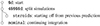 |
Fig. 1. Overview of the simulations in this work. The steroids model starts at t = 40 000 d from the nominal model with the guess of the final state obtained via the method outlined in Appendix B. |
The steroids model has been initialized from the nominal model at t = 40 000 d. The initialization of the steroids model is done by extrapolating the temperature evolution of the nominal model using log-linear regression. The extrapolation to find the steroids model resembles a hotter limit on the prediction from the temperature evolution of the nominal model up until t = 40 000 d, while we take over the dynamical state (e.g., the velocity field). We explain the details of the fit and initialization in Appendix B.
3. Results from nongray 3D GCM
Utilizing the performance of expeRT/MITgcm, we monitor the temperature convergence of WASP-76 b up to t = 86000 d. We show the final atmospheric state and observables in Appendix C. The horizontally averaged thermal profile for pressures above p = 0.1 bar is shown in Fig. 2. The nominal model cools down from an initially hot state to an almost stable solution within 30 000 d, where the temperature changes at the bottom boundary become smaller than 0.1 K d−1, as shown in Fig. 3. However, the temperature of the model continues to decrease further and will reach a much colder state within reasonable timescales. Structure models such as those of Thorngren et al. (2019) and Sarkis et al. (2021) often give predictions about the location of the radiative convective boundary (RCB), defined as the first pressure layer from the bottom upwards, where the temperature becomes subadiabatic (Thorngren et al. 2019). For better comparison of our model to those predictions, we calculate the RCB in the same way, and show this as gray dots in Fig. 2.
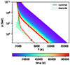 |
Fig. 2. Temperature evolution (color coded) of the horizontally averaged temperature in the deep layers of the atmosphere for the nominal model (solid lines) and the steroids model (dotted lines). A gray dot displays the position of the RCB at the final state. |
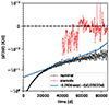 |
Fig. 3. Evolution of the rate of temperature change at 650 bar with time of the nominal (black) and the steroids (red) model. We note that the y-axis is linear between −0.01 and 0.01 and logarithmic elsewhere. The fit on the rate of temperature change by an exponential decay around t = 40 000 d is shown in blue. |
We fitted the temperature evolution around 40 000 day in order to estimate how much colder the final state would be. Assuming an exponential decay of the temperature changes with time, we estimated the final temperature at p = 650 bar to be T = 4567 K (Appendix B). We performed a second simulation (dubbed steroids) using this final state as an initial condition to monitor the stability of such a model. The resulting temperature evolution of this model is shown as dotted lines in Fig. 2. The new initial state seems to be a good initial guess in the deep layers, whereas some adjustment happens in intermediate layers between 0.1 bar and 100 bar. Looking at the temperature change rates (Fig. 3), we find that the temperature reaches a steady state, where the temperature stops changing, and the temperature changes start to swap signs in an oscillating manner with ≈5 × 10⁻³ K d−1. We therefore claim that temperature convergence has been reached in the steroids model, implying that the temperature of our WASP-76 b models self-consistently converges to a cold interior.
The planet gains energy from stellar irradiation and loses energy by thermal radiation. We can therefore formulate the energy balance as an integral over the net radiative flux Ftot as
 (2)
(2)
where ϑ and φ are latitude and longitude respectively, Tint[K] is the intrinsic temperature and Rpla is the planetary radius. Here, Fpla and F⋆ are the planetary and stellar fluxes, respectively. In radiative equilibrium, without an internal energy source, it should hold that
 (3)
(3)
and subsequently Tint = 0 K from Eq. (2). We note that we do not impose a nonzero flux as the boundary condition of the radiative transfer in our GCM. Instead, the boundary condition for the thermal flux at the deepest layer of the atmosphere is zero, which corresponds to Tint = 0 K.
We display the effect of the intrinsic temperature on the temperature profile in Fig. 4, where we show temperature profiles with three different intrinsic temperatures (500 K, 600 K, and 700 K) along with the final time steps of the steroids and nominal model from Fig. 2. The temperature profiles for the different intrinsic temperatures have been calculated from the temperature evolution of the nominal model (Fig. 2) using Eq. (2) with bolometric fluxes, which was computed during the runtime of the climate simulations. The steroids model has a negative total net flux, rendering it impossible to calculate a physical meaningful intrinsic temperature.
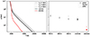 |
Fig. 4. Temperature profiles and RCB locations. Left: temperature profiles for different intrinsic temperatures (gray) and final temperature profiles of the nominal (Tint ≈ 434 K) and steroids simulation. Right: calculated RCB for the different temperature profiles of the left panel. Additional markers display the RCB calculated for the equatorial and the polar region. The gray profiles are calculated from the temperature evolution of the nominal model. We note that the steroids model loses energy due to dissipation and therefore has no physical intrinsic temperature. |
Combining the predictions from Thorngren et al. (2019) and Sarkis et al. (2021), we find that the intrinsic temperature of WASP-76 b should be approximately 600 ± 100 K and the RCB location should be 1 ± 1 bar according to structure models. Thus, we can compare the intrinsic temperature to the predictions and find that the intrinsic temperature of the final nominal model is 434 K, which is significantly below the predicted value of 600 K from structure models.
The right plot in Fig. 4 displays the RCB location for the same models. Comparing the RCB location of the final globally averaged nominal and steroids model to the predictions from the above-mentioned 1D structure models, we find that the locations of the RCB in our models are much deeper than 10 bar, and therefore not in line with predictions. Rauscher & Showman (2014) showed that the RCB location varies horizontally, because the equatorial regions have higher stellar fluxes than the polar regions. We therefore performed additional calculations of the RCB with temperature averages of the polar (|ϑ|> 45°) and equatorial (|ϑ|< 45°) regions. We can confirm the findings of Rauscher & Showman (2014), namely that the RCB location seems to vary horizontally, where we find higher and deeper levels for polar and equatorial regions, respectively. The different values of the RCB for different horizontal regions is caused by the fact that the temperature becomes horizontally homogeneous only at deeper levels in the atmosphere. We therefore conclude that the intrinsic model differences of 1D and 3D models make the comparison of RCB locations more difficult.
We show the evolution of the area-integrated radiative fluxes (F⋆ and Fpla) along with the total energy of the steroids and nominal in Fig. 5. We follow Polichtchouk et al. (2014) and calculate the total energy (TE) as a sum of the potential, kinetic, and internal energy by
 (4)
(4)
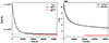 |
Fig. 5. Energy budget of the nominal and steroids simulations. Left: radiative energy budget (∫FdA). Right: evolution of the total energy. Both simulations converge toward radiative equilibrium with approximately 0.1% accuracy. |
where Z is the geometric height. The plot shows that the high temperatures in the deep atmosphere do not lead to large flux differences between the stellar and planetary fluxes, which can be explained by the relation between flux and temperature, which goes with the fourth power of the temperature (Eq. (2)). Intrinsic temperatures on the order of 1000 K therefore become insignificant against the temperature of the thermal emission, which is on the order of 2000 K. The nominal model loses energy during its evolution as the planet cools down, whereas the steroids model heats up again slightly. These trends manifest themselves in the right panel of Fig. 5, showing that the steroids model conserves the total energy, whereas the nominal model is still losing energy through radiation to space.
Our model conserves the radiative energy to roughly 99.9%. Deitrick et al. (2022) recently reported that in practice their THOR GCM always tends toward a negative radiative flux balance, with discrepancies of as large as a few percent. The authors claim that the reason for that can be found in the numerical dissipation processes in their model such as sponge layers and hyper-diffusion2. Similarly, Rauscher & Menou (2012) report that their total radiative heating rate is always positive, balancing a loss of kinetic energy due to numerics. The conservation of energy and angular momentum in MITgcm was benchmarked by Polichtchouk et al. (2014), revealing that MITgcm is particularly poor at conserving angular momentum, whereas it performs well at conserving energy, which can be confirmed for the steroids model in the right panel of Fig. 5. We therefore think that conservation of the radiative energy with an accuracy of 99.9% is already very good. It is therefore perfectly reasonable that the steroids model is indeed losing more energy than it is gaining, while still being in equilibrium.
4. Discussion
We conclude that we cannot find large-scale atmospheric motions able to inflate a planet significantly. Instead, we find that heating and cooling by radiation dominate the temperature evolution even in deep layers, forcing our nongray simulations toward a cool final state. We therefore propose that hydrodynamical models of hot gas giants need extra physics or parameterization (such as dissipative drag or diffusion) to recreate an inflated interior.
Youdin & Mitchell (2010) and Tremblin et al. (2017) showed that vertical heat transport by turbulent mixing could possibly inflate the interior. However, their models do not model vertical mixing self-consistently, instead relying on a parameter that sets the mixing strength. Using idealized GCM simulations, Sainsbury-Martinez et al. (2019) claimed that large-scale atmospheric motions could be a reason for a tendency toward a hot adiabatic interior in their simulations. There are two major differences between the model used in this work and the GCM used in the work of these latter authors that need to be considered when questioning the lack of a hot interior in our models in comparison to their work. One of the obvious differences is the treatment of radiation: whereas Sainsbury-Martinez et al. (2019) do not include radiative cooling and heating in the deep atmosphere, we apply a nongray radiative transfer scheme.
Perhaps equally as important, the second difference is the use of numerical dissipation, where Sainsbury-Martinez et al. (2019) use a hyper-diffusion scheme to stabilize their model, whereas we use a fourth-order Shapiro filter. Previous studies showed that in general, both dissipation schemes (filtering and diffusion) have a profound influence on the temperature and dynamics of a GCM (e.g., Polichtchouk et al. 2014; Koll & Komacek 2018; Hammond & Abbot 2022). Sainsbury-Martinez et al. (2019) showed that the strength of numerical diffusion in their model critically impacts the timescale of the tendency toward the hot adiabat, where a strong numerical diffusion relates to a faster evolution toward a hot interior. It could therefore be possible that their finding might have been caused by heat diffusion from their numerical dissipation scheme.
It is still unclear how the interior of hot and ultra-hot Jupiters interact with the upper atmosphere. There are currently few studies that link the convective interior with the photosphere dynamics (Showman et al. 2020). The first steps toward this goal were made by Lian et al. (2022), who model the effect of convective forcing on the circulation patterns of hot irradiated planets with a combination of Newtonian forcing in the upper atmosphere and perturbations in the deep atmosphere. A model able to combine 1D interior models with realistic 3D atmospheric models including radiative transfer would also be desirable and would reveal insights into the connection between the convection in the deep interior and the atmosphere. Similar approaches, connecting convective interiors with upper radiative atmospheres, exist in the stellar community (e.g., Skartlien et al. 2000; Freytag et al. 2010, 2017, 2019).
The present work is the most complete GCM study to date, which is aimed at understanding the coupling of the upper and the deeper atmosphere in hot Jupiters. However, we note that we are so far omitting important effects for ultra-hot Jupiters: Ohmic dissipation, dissociation of H2 and clouds. The upper atmospheres of ultra-hot Jupiters like WASP-76b are highly ionized due to their high temperatures (e.g., Helling et al. 2021). Magnetic fields, if present, would therefore couple strongly to the ionized winds. Rauscher & Menou (2013) and Beltz et al. (2022) showed that friction induced by magnetic fields acting on ionized winds may alter the dynamical state of the atmosphere and lead to additional heating in the upper atmosphere, where friction is converted to heat. It is still debated and unclear (Rauscher & Menou 2013; Showman et al. 2020) as to whether this extra heat could be sufficient to inflate a planet.
Recent simulations of ultra-hot Jupiters showed that H2 dissociation can alter their thermal structure (Tan & Komacek 2019). The energy needed to dissociate molecular hydrogen on the day side cools the atmosphere, while recombination of atomic hydrogen heats the night side, leading to an overall reduced day–night temperature contrast. Similarly, the presence of clouds in a 3D GCM will alter the thermal and dynamical state of hot Jupiters (Roman et al. 2021; Deitrick et al. 2022). Realistic models of ultra-hot Jupiters should therefore take these effects into account, even though it is unlikely that these effects are important for the deeper parts of the atmosphere.
5. Summary and conclusions
In this work, we investigate one of the main hypotheses proposed by Guillot & Showman (2002) and Youdin & Mitchell (2010) to explain the abnormally large radii of inflated hot Jupiters: Energy transport from the irradiated atmosphere into deeper layers. We performed long-term (86 000 d) nongray 3D GCM simulations of WASP-76 b to search for signs of vertical advection of potential temperature from the upper irradiated atmosphere into the interior. Our simulations started from a hot initial state and cooled down toward a colder state. We then used an exponential fit on the temperature convergence to extrapolate the temperature toward a possible final converged state, which was reached soon after for the extrapolated simulation. The final converged simulation exhibits a cold temperature profile, lacking signs of vertical advection of heat from the upper atmosphere into the interior. We find instead that the atmosphere has cooled down to radiative equilibrium, conserving energy with an accuracy of 99.9%.
Our work strongly disfavors vertical downward advection of energy from the irradiated part of the atmosphere by large-scale atmospheric circulation as a possible explanation for inflation. We suggest instead that physical processes other than radiation and dynamics need to be taken into account in order to match the abnormal large radii of inflated hot Jupiters. Such processes could be the interaction between a convective interior and the atmosphere, small-scale turbulent transport, or magnetic field interactions. Future investigations are needed to quantify3 their effects on the state of radius inflation4.
We note that all GCMs need some form of dissipation for numerical reasons (Jablonowski et al. 2011).
available at: https://prt-phasecurve.readthedocs.io/en/latest/
Acknowledgments
We thank Xianyu Tan for fruitful discussions on the effect of numerical dissipation on the thermal structure of GCM simulations. We also thank an anonymous referee for their useful comments that improved the quality of the manuscript. A.D.S., L.D., U.G.J and C.H. acknowledge funding from the European Union H2020-MSCA-ITN-2019 under Grant no. 860470 (CHAMELEON). L.C. acknowledges the Royal Society University Fellowship URF R1 211718 hosted by the University of St Andrews. U.G.J acknowledges funding from the Novo Nordisk Foundation Interdisciplinary Synergy Program grant no. NNF19OC0057374. The bibliography of this publication has been typesetted using bibmanager (Cubillos 2020). The post-processing of GCM data has been performed with gcm-toolkit (Schneider et al. 2022).
References
- Adcroft, A., Campin, J.-M., Hill, C., & Marshall, J. 2004, Mon. Weather Rev., 132, 2845 [NASA ADS] [CrossRef] [Google Scholar]
- Arras, P., & Socrates, A. 2010, ApJ, 714, 1 [Google Scholar]
- Azzam, A. A. A., Tennyson, J., Yurchenko, S. N., & Naumenko, O. V. 2016, MNRAS, 460, 4063 [NASA ADS] [CrossRef] [Google Scholar]
- Barber, R. J., Strange, J. K., Hill, C., et al. 2014, MNRAS, 437, 1828 [CrossRef] [Google Scholar]
- Batygin, K., & Stevenson, D. J. 2010, ApJ, 714, L238 [NASA ADS] [CrossRef] [Google Scholar]
- Beltz, H., Rauscher, E., Roman, M. T., & Guilliat, A. 2022, AJ, 163, 35 [NASA ADS] [CrossRef] [Google Scholar]
- Bodenheimer, P., Lin, D. N. C., & Mardling, R. A. 2001, ApJ, 548, 466 [NASA ADS] [CrossRef] [Google Scholar]
- Borysow, A. 2002, A&A, 390, 779 [NASA ADS] [CrossRef] [EDP Sciences] [Google Scholar]
- Borysow, A., & Frommhold, L. 1989, ApJ, 341, 549 [NASA ADS] [CrossRef] [Google Scholar]
- Borysow, J., Frommhold, L., & Birnbaum, G. 1988, ApJ, 326, 509 [NASA ADS] [CrossRef] [Google Scholar]
- Borysow, A., Frommhold, L., & Moraldi, M. 1989, ApJ, 336, 495 [NASA ADS] [CrossRef] [Google Scholar]
- Borysow, A., Jorgensen, U. G., & Fu, Y. 2001, J. Quant. Spectr. Rad. Transf., 68, 235 [NASA ADS] [CrossRef] [Google Scholar]
- Carone, L., Baeyens, R., Mollière, P., et al. 2020, MNRAS, 496, 3582 [NASA ADS] [CrossRef] [Google Scholar]
- Carone, L., Mollière, P., Zhou, Y., et al. 2021, A&A, 646, A168 [NASA ADS] [CrossRef] [EDP Sciences] [Google Scholar]
- Chan, Y. M., & Dalgarno, A. 1965, Proc. Phys. Soc., 85, 227 [NASA ADS] [CrossRef] [Google Scholar]
- Coles, P. A., Yurchenko, S. N., & Tennyson, J. 2019, MNRAS, 490, 4638 [CrossRef] [Google Scholar]
- Cubillos, P. E. 2020, https://doi.org/10.5281/zenodo.3634059 [Google Scholar]
- Dalgarno, A., & Williams, D. A. 1962, ApJ, 136, 690 [NASA ADS] [CrossRef] [Google Scholar]
- Deitrick, R., Heng, K., Schroffenegger, U., et al. 2022, MNRAS, 512, 3759 [NASA ADS] [CrossRef] [Google Scholar]
- Ehrenreich, D., Lovis, C., Allart, R., et al. 2020, Nature, 580, 597 [Google Scholar]
- Fortney, J. J., Dawson, R. I., & Komacek, T. D. 2021, J. Geophys. Res. (Planets), 126, e06629 [NASA ADS] [Google Scholar]
- Freytag, B., Allard, F., Ludwig, H. G., Homeier, D., & Steffen, M. 2010, A&A, 513, A19 [NASA ADS] [CrossRef] [EDP Sciences] [Google Scholar]
- Freytag, B., Liljegren, S., & Höfner, S. 2017, A&A, 600, A137 [NASA ADS] [CrossRef] [EDP Sciences] [Google Scholar]
- Freytag, B., Höfner, S., & Liljegren, S. 2019, IAU Symp., 343, 9 [NASA ADS] [Google Scholar]
- Ginzburg, S., & Sari, R. 2015, ApJ, 803, 111 [NASA ADS] [CrossRef] [Google Scholar]
- Gray, D. F. 2008, The Observation and Analysis of Stellar Photospheres [Google Scholar]
- Guillot, T., & Showman, A. P. 2002, A&A, 385, 156 [NASA ADS] [CrossRef] [EDP Sciences] [Google Scholar]
- Hammond, M., & Abbot, D. S. 2022, MNRAS, 511, 2313 [NASA ADS] [CrossRef] [Google Scholar]
- Helling, C., Worters, M., Samra, D., Molaverdikhani, K., & Iro, N. 2021, A&A, 648, A80 [NASA ADS] [CrossRef] [EDP Sciences] [Google Scholar]
- Heng, K., Menou, K., & Phillipps, P. J. 2011, MNRAS, 413, 2380 [NASA ADS] [CrossRef] [Google Scholar]
- Jablonowski, C., & Williamson, D. L. 2011, in The Pros and Cons of Diffusion, Filters and Fixers in Atmospheric General Circulation Models, eds. P. Lauritzen, C. Jablonowski, M. Taylor, & R. Nair (Berlin, Heidelberg: Springer), 381 [Google Scholar]
- Kesseli, A. Y., & Snellen, I. A. G. 2021, ApJ, 908, L17 [Google Scholar]
- Kesseli, A. Y., Snellen, I. A. G., Casasayas-Barris, N., Mollière, P., & Sánchez-López, A. 2022, AJ, 163, 107 [NASA ADS] [CrossRef] [Google Scholar]
- Knierim, H., Batygin, K., & Bitsch, B. 2022, A&A, 658, L7 [NASA ADS] [CrossRef] [EDP Sciences] [Google Scholar]
- Koll, D. D. B., & Komacek, T. D. 2018, ApJ, 853, 133 [NASA ADS] [CrossRef] [Google Scholar]
- Li, G., Gordon, I. E., Rothman, L. S., et al. 2015, ApJS, 216, 15 [NASA ADS] [CrossRef] [Google Scholar]
- Lian, Y., Showman, A. P., Tan, X., & Hu, Y. 2022, ApJ, 928, 166 [NASA ADS] [CrossRef] [Google Scholar]
- May, E. M., Komacek, T. D., Stevenson, K. B., et al. 2021, AJ, 162, 158 [NASA ADS] [CrossRef] [Google Scholar]
- Mayne, N. J., Debras, F., Baraffe, I., et al. 2017, A&A, 604, A79 [NASA ADS] [CrossRef] [EDP Sciences] [Google Scholar]
- McKemmish, L. K., Yurchenko, S. N., & Tennyson, J. 2016, MNRAS, 463, 771 [NASA ADS] [CrossRef] [Google Scholar]
- McKemmish, L. K., Masseron, T., Hoeijmakers, H. J., et al. 2019, MNRAS, 488, 2836 [Google Scholar]
- Menou, K. 2012, ApJ, 745, 138 [NASA ADS] [CrossRef] [Google Scholar]
- Mollière, P., Wardenier, J. P., van Boekel, R., et al. 2019, A&A, 627, A67 [Google Scholar]
- Mollière, P., Stolker, T., Lacour, S., et al. 2020, A&A, 640, A131 [Google Scholar]
- Perna, R., Menou, K., & Rauscher, E. 2010, ApJ, 719, 1421 [NASA ADS] [CrossRef] [Google Scholar]
- Piskunov, N. E., Kupka, F., Ryabchikova, T. A., Weiss, W. W., & Jeffery, C. S. 1995, A&AS, 112, 525 [Google Scholar]
- Polichtchouk, I., Cho, J. Y. K., Watkins, C., et al. 2014, Icarus, 229, 355 [NASA ADS] [CrossRef] [Google Scholar]
- Polyansky, O. L., Kyuberis, A. A., Zobov, N. F., et al. 2018, MNRAS, 480, 2597 [NASA ADS] [CrossRef] [Google Scholar]
- Rauscher, E., & Menou, K. 2012, ApJ, 750, 96 [NASA ADS] [CrossRef] [Google Scholar]
- Rauscher, E., & Menou, K. 2013, ApJ, 764, 103 [NASA ADS] [CrossRef] [Google Scholar]
- Rauscher, E., & Showman, A. P. 2014, ApJ, 784, 160 [NASA ADS] [CrossRef] [Google Scholar]
- Richard, C., Gordon, I. E., Rothman, L. S., et al. 2012, J. Quant. Spectr. Rad. Transf., 113, 1276 [Google Scholar]
- Roman, M. T., Kempton, E. M. R., Rauscher, E., et al. 2021, ApJ, 908, 101 [CrossRef] [Google Scholar]
- Sainsbury-Martinez, F., Wang, P., Fromang, S., et al. 2019, A&A, 632, A114 [NASA ADS] [CrossRef] [EDP Sciences] [Google Scholar]
- Sainsbury-Martinez, F., Casewell, S. L., Lothringer, J. D., Phillips, M. W., & Tremblin, P. 2021, A&A, 656, A128 [NASA ADS] [CrossRef] [EDP Sciences] [Google Scholar]
- Sarkis, P., Mordasini, C., Henning, T., Marleau, G. D., & Mollière, P. 2021, A&A, 645, A79 [NASA ADS] [CrossRef] [EDP Sciences] [Google Scholar]
- Savel, A. B., Kempton, E. M. R., Malik, M., et al. 2022, ApJ, 926, 85 [NASA ADS] [CrossRef] [Google Scholar]
- Schneider, A. D., Baeyens, R., & Kiefer, S. 2022, https://doi.org/10.5281/zenodo.7116787 [Google Scholar]
- Schneider, A. D., Carone, L., Decin, L., et al. 2022, A&A, 664, A56 [NASA ADS] [CrossRef] [EDP Sciences] [Google Scholar]
- Seidel, J. V., Ehrenreich, D., Wyttenbach, A., et al. 2019, A&A, 623, A166 [NASA ADS] [CrossRef] [EDP Sciences] [Google Scholar]
- Showman, A. P., Fortney, J. J., Lian, Y., et al. 2009, ApJ, 699, 564 [NASA ADS] [CrossRef] [Google Scholar]
- Showman, A. P., Tan, X., & Parmentier, V. 2020, Space Sci. Rev., 216, 139 [Google Scholar]
- Skartlien, R., Stein, R. F., & Nordlund, Å. 2000, ApJ, 541, 468 [Google Scholar]
- Skinner, J. W., & Cho, J. Y. K. 2021, MNRAS, 504, 5172 [NASA ADS] [CrossRef] [Google Scholar]
- Socrates, A. 2013, ArXiv e-prints [arXiv:1304.4121] [Google Scholar]
- Sousa-Silva, C., Al-Refaie, A. F., Tennyson, J., & Yurchenko, S. N. 2015, MNRAS, 446, 2337 [Google Scholar]
- Tan, X., & Komacek, T. D. 2019, ApJ, 886, 26 [Google Scholar]
- Thorngren, D. P., & Fortney, J. J. 2018, AJ, 155, 214 [Google Scholar]
- Thorngren, D., Gao, P., & Fortney, J. J. 2019, ApJ, 884, L6 [Google Scholar]
- Tremblin, P., Chabrier, G., Mayne, N. J., et al. 2017, ApJ, 841, 30 [NASA ADS] [CrossRef] [Google Scholar]
- Wardenier, J. P., Parmentier, V., Lee, E. K. H., Line, M. R., & Gharib-Nezhad, E. 2021, MNRAS, 506, 1258 [NASA ADS] [CrossRef] [Google Scholar]
- Wende, S., Reiners, A., Seifahrt, A., & Bernath, P. F. 2010, A&A, 523, A58 [NASA ADS] [CrossRef] [EDP Sciences] [Google Scholar]
- West, R. G., Hellier, C., Almenara, J. M., et al. 2016, A&A, 585, A126 [NASA ADS] [CrossRef] [EDP Sciences] [Google Scholar]
- Youdin, A. N., & Mitchell, J. L. 2010, ApJ, 721, 1113 [NASA ADS] [CrossRef] [Google Scholar]
- Yurchenko, S. N., Amundsen, D. S., Tennyson, J., & Waldmann, I. P. 2017, A&A, 605, A95 [NASA ADS] [CrossRef] [EDP Sciences] [Google Scholar]
- Yurchenko, S. N., Mellor, T. M., Freedman, R. S., & Tennyson, J. 2020, MNRAS, 496, 5282 [NASA ADS] [CrossRef] [Google Scholar]
Appendix A: Effect of the drag
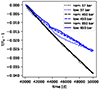 |
Fig. A.1. Evolution of the temperature in three pressure layers (57 bar, 450 bar, 650 bar) in a simulation with low drag compared to the nominal simulation. The temperature in each layer is normed to the respective initial value at 40 000 d. |
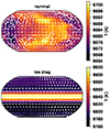 |
Fig. A.2. Isobaric temperature slices at t = 50000 d at p = 650 bar for the nominal and the model with low drag. The temperature has been averaged over the last 100 d. The substellar point is located in the center of the plot. |
Previous studies revealed the enormous impact of the chosen (often unjustified) dissipation schemes (Heng et al. 2011; Skinner & Cho 2021). We perform a test simulation with a 1000 times longer friction timescale (τdeep) compared to the nominal and steroids simulations. This longer friction timescale weakens the strength of the Rayleigh drag applied to the deep atmosphere and makes sure that the prescription of the bottom drag does not affect the conclusions of this work. This additional simulation has been started from the nominal model at 40 000 d and has been carried out for 10000 d.
We compare the temperature evolution of the nominal simulation to the simulation with the low drag in Fig. A.1, where we find that the simulation with the lower drag cools down slower than the nominal simulation. The reason for the difference in the temperature evolution can be found in the Fig. A.2, where we show the temperature maps at 650 bar of the model with low drag and the nominal model. Both models start from an average temperature of 10 080 K at 40 000 d and cool down by a few hundred Kelvin. However, we find that the drag stops the equatorial jet, which otherwise descends toward the bottom boundary in the simulation with low drag. Simultaneously, stopping the equatorial jet leads to an efficient north–south redistribution of the temperature at the bottom boundary. Thus, in the model with much smaller drag, we find that the temperature starts diverging between the poles and the equator, where the equator cools down slower than the poles.
Considering this result, it is reasonable to conclude that the final converged solution of a model with lower drag would be hotter than the steroids model, possibly reducing the gap between outgoing and incoming radiation in the left panel of Fig. 5. Nevertheless, we also find that this simulation continues to cool down, still showing no sign of the vertical advection of heat that would, on the contrary, lead to a warming of the deep layers.
Appendix B: Prediction of the final state of the atmosphere
Temperature convergence in the deep layers of the atmospheres of hot Jupiters is impossible to reach in reasonable model runtimes. We therefore propose to speed up convergence by predicting the final converged state and extrapolating to this final state, which can then be used to initialize a new model. The method outlined below is one possible approach to doing this. In order to be able to predict the final state of the temperature in the deep atmosphere, we apply three assumptions:
-
The temperature in the deep atmosphere is horizontally isotropic and homogeneous.
-
The temperature decrease can be modeled by an exponential decay.
-
The deep layers are adiabatic:
 .
.
We note that these assumptions (especially the second) are rather too simplified to capture the actual cooling of planets, which is not thought to be consistent over time (Ginzburg & Sari 2015). However, these simplifications do not need to be true, because their only purpose is to predict the initial state of the steroids model. Moreover, in order to minimize temporal variations unrelated to the general trend of temperature convergence, we compute the horizontally and temporally averaged temperature over a sampling period of 1000 d. We perform this computation for four sampling periods (e.g., for a total of 4000 d) yielding four values for the potential temperature of four consecutive sampling periods. This computation is done in retrograde at t = 40 000 d with the 100 d time-averaged temperature fields from 36 000 d to 40 000 d.
We then use the least-squares method to fit a linear relation
 (B.1)
(B.1)
where λ is a norm that ensures that the value inside log stays positive and unitless. We set
 (B.2)
(B.2)
the subscripts i, j ∈ {1, 2, 3, 4} to denote the four support points of the fit. We can now use the least-squares method to solve
 (B.3)
(B.3)
in order to obtain the best-fit values for m and c, which is equivalent to
 (B.4)
(B.4)
where c̃ = exp(c). The fit, as displayed in Fig. 3, matches the temperature change rates around t = 40 000 d. However, the real temperature change rates for later times are slightly below the fit, meaning that the temperature cools down even faster than predicted by the fit.
We then estimate the final temperature from integrating Eq. (B.4) over time and get
 (B.5)
(B.5)
We evaluate this equation at the age of the mother star, which is ≈5 Gyr (West et al. 2016), and find that the temperature at 650 bar should be T650 bar = 4567 K. This temperature at the bottom of the simulation domain is then translated to an adiabatic temperature profile for the atmospheric layers below 10 bar and is used to kick off the steroids model.
In order to force the simulation to continue with this new temperature profile for pressure levels below 10 bar, we developed a method that would smoothly force the temperature towards the predicted state during runtime. This method consists of a time-based smoothing, where the temperature is forced towards the final state by splitting the total change of temperature over a period of 10 d. We make sure that the temperature is changed by the expected amount, but still modulate the change rates by a sine function  to smoothen the transition. A linear vertical smoothing between 1 bar and 10 bar ensures that the upper atmosphere above 1 bar stays untouched from the artificial forcing, which should only change the temperature in the deep layers. These measures are only used for the period of 10 day, and their only purpose is to force the temperature of the steroids model towards its new initial condition. The temperature forcing after 40010 d is then given by standard radiative heating and cooling as computed self-consistently within the GCM.
Appendix C: Models of WASP-76b
We found in Schneider et al. (2022) that the influence of the deep atmospheric state on the temperature profile in the upper atmospheric layers is very limited. As we see in Fig. 2, the global average of the temperature in the steroids and nominal model only diverges for pressures above 1 bar. We show an isobaric map of the temperature at 1 bar in Fig. C.1, where we can see that the steroid and nominal model look similar, yet not identical. This becomes especially apparent in the plots of the zonal mean of the zonal wind velocity in Fig. C.2. The winds in the steroids model are much stronger than the winds in the nominal model. This will have an observable impact, resulting in higher hot spot offsets and greatly impacting high-resolution Doppler observations.
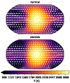 |
Fig. C.1. Final isobaric temperature-slices at p ≈ 1.2 bar for the nominal and steroids model. The temperature has been averaged over the last 100 d. The substellar point is located in the center of the plot. |
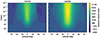 |
Fig. C.2. Zonal mean eastward velocity for the nominal and the steroids model. |
These strong differences in wind speed were not observed in the simulations of Schneider et al. (2022), where we did not compare models with such differences in temperature. The transition to higher wind speeds might be caused by the increase in the weather layer, which is caused by larger (relative) horizontal anisotropies in the deep atmosphere, which affects the jet strength (Mayne et al. 2017). However, we note that the kinetic energy makes up less than 1% of the energy budget in our models. It is therefore also possible that the reason for the differences is simply rooted in the particularly poor conservation of angular momentum in MITgcm (Polichtchouk et al. 2014). Further study is needed to entangle the dynamical differences in models with cold and hot interiors.
To quantify the hot spot offset, we computed phase curves using prt_phasecurve5. prt_phasecurve computes 288 intensity fields at the top of the atmosphere using petitRADTRANS (Mollière et al. 2019, 2020) on a longitude latitude grid with 15° resolution and for 20 angles instead of the nominal 3 angles that petitRADTRANS uses. These individual spectra are then integrated by taking the individual angles into account (i.e., without the assumption of isotropic irradiation).
The difference in the offset shift can be seen in the thermal phase curve in Fig. C.3. The overall shape of the phase curves in the nominal and steroids model is very similar. However, we can see that the day–night contrast is higher in the case of the nominal model, which can be explained by the strong winds in the steroids model that are more efficient in equilibrating the temperature in the steroids model. Similarly, we can see that the hot spot offset is greater in the steroids model, which is another outcome of the strong winds that transport energy further, before it can be reradiated.
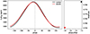 |
Fig. C.3. Phase curve and phase offset. Left: Phase curve at λ = 4.5 μm, computed using prt_phasecurve. The dashed gray line corresponds to the center of the dayside. Right: Difference between the dayside center and the maximum of the phase curve. |
All Figures
|
Fig. 1. Overview of the simulations in this work. The steroids model starts at t = 40 000 d from the nominal model with the guess of the final state obtained via the method outlined in Appendix B. |
| In the text | |
|
Fig. 2. Temperature evolution (color coded) of the horizontally averaged temperature in the deep layers of the atmosphere for the nominal model (solid lines) and the steroids model (dotted lines). A gray dot displays the position of the RCB at the final state. |
| In the text | |
|
Fig. 3. Evolution of the rate of temperature change at 650 bar with time of the nominal (black) and the steroids (red) model. We note that the y-axis is linear between −0.01 and 0.01 and logarithmic elsewhere. The fit on the rate of temperature change by an exponential decay around t = 40 000 d is shown in blue. |
| In the text | |
|
Fig. 4. Temperature profiles and RCB locations. Left: temperature profiles for different intrinsic temperatures (gray) and final temperature profiles of the nominal (Tint ≈ 434 K) and steroids simulation. Right: calculated RCB for the different temperature profiles of the left panel. Additional markers display the RCB calculated for the equatorial and the polar region. The gray profiles are calculated from the temperature evolution of the nominal model. We note that the steroids model loses energy due to dissipation and therefore has no physical intrinsic temperature. |
| In the text | |
|
Fig. 5. Energy budget of the nominal and steroids simulations. Left: radiative energy budget (∫FdA). Right: evolution of the total energy. Both simulations converge toward radiative equilibrium with approximately 0.1% accuracy. |
| In the text | |
|
Fig. A.1. Evolution of the temperature in three pressure layers (57 bar, 450 bar, 650 bar) in a simulation with low drag compared to the nominal simulation. The temperature in each layer is normed to the respective initial value at 40 000 d. |
| In the text | |
|
Fig. A.2. Isobaric temperature slices at t = 50000 d at p = 650 bar for the nominal and the model with low drag. The temperature has been averaged over the last 100 d. The substellar point is located in the center of the plot. |
| In the text | |
|
Fig. C.1. Final isobaric temperature-slices at p ≈ 1.2 bar for the nominal and steroids model. The temperature has been averaged over the last 100 d. The substellar point is located in the center of the plot. |
| In the text | |
|
Fig. C.2. Zonal mean eastward velocity for the nominal and the steroids model. |
| In the text | |
|
Fig. C.3. Phase curve and phase offset. Left: Phase curve at λ = 4.5 μm, computed using prt_phasecurve. The dashed gray line corresponds to the center of the dayside. Right: Difference between the dayside center and the maximum of the phase curve. |
| In the text | |
Current usage metrics show cumulative count of Article Views (full-text article views including HTML views, PDF and ePub downloads, according to the available data) and Abstracts Views on Vision4Press platform.
Data correspond to usage on the plateform after 2015. The current usage metrics is available 48-96 hours after online publication and is updated daily on week days.
Initial download of the metrics may take a while.