| Issue |
A&A
Volume 666, October 2022
|
|
|---|---|---|
| Article Number | A76 | |
| Number of page(s) | 14 | |
| Section | Numerical methods and codes | |
| DOI | https://doi.org/10.1051/0004-6361/202243469 | |
| Published online | 11 October 2022 | |
Multiscale entropy analysis of astronomical time series
Discovering subclusters of hybrid pulsators
1
Institute of Astronomy, KU Leuven,
Celestijnenlaan 200D,
3001
Leuven, Belgium
e-mail: This email address is being protected from spambots. You need JavaScript enabled to view it.
2
Department of Physics and Kavli Institute for Astrophysics and Space Research, Massachusetts Institute of Technology,
Cambridge, MA
02139, USA
Received:
3
March
2022
Accepted:
20
June
2022
Abstract
Context. The multiscale entropy assesses the complexity of a signal across different timescales. It originates from the biomedical domain and was recently successfully used to characterize light curves as part of a supervised machine learning framework to classify stellar variability.
Aims. We aim to explore the behavior of the multiscale entropy in detail by studying its algorithmic properties in a stellar variability context and by linking it with traditional astronomical time series analysis methods and metrics such as the Lomb-Scargle periodogram. We subsequently use the multiscale entropy as the basis for an interpretable clustering framework that can distinguish hybrid pulsators with both p- and g-modes from stars with only p-mode pulsations, such as δ Scuti (δ Sct) stars, or from stars with only g-mode pulsations, such as γ Doradus (γ Dor) stars.
Methods. We calculate the multiscale entropy for a set of Kepler light curves and simulated sine waves. We link the multiscale entropy to the type of stellar variability and to the frequency content of a signal through a correlation analysis and a set of simulations. The dimensionality of the multiscale entropy is reduced to two dimensions and is subsequently used as input to the HDBSCAN density-based clustering algorithm in order to find the hybrid pulsators within sets of δ Sct and γ Dor stars that were observed by Kepler.
Results. We find that the multiscale entropy is a powerful tool for capturing variability patterns in stellar light curves. The multiscale entropy provides insights into the pulsation structure of a star and reveals how short- and long-term variability interact with each other based on time-domain information only. We also show that the multiscale entropy is correlated to the frequency content of a stellar signal and in particular to the near-core rotation rates of g-mode pulsators. We find that our new clustering framework can successfully identify the hybrid pulsators with both p- and g-modes in sets of δ Sct and γ Dor stars, respectively. The benefit of our clustering framework is that it is unsupervised. It therefore does not require previously labeled data and hence is not biased by previous knowledge.
Key words: asteroseismology / methods: data analysis / methods: observational / methods: statistical / techniques: photometric
© J. Audenaert and A. Tkachenko 2022
 Open Access article, published by EDP Sciences, under the terms of the Creative Commons Attribution License (https://creativecommons.org/licenses/by/4.0), which permits unrestricted use, distribution, and reproduction in any medium, provided the original work is properly cited.
This article is published in open access under the Subscribe-to-Open model. This email address is being protected from spambots. You need JavaScript enabled to view it. to support open access publication.
1 Introduction
The light curve of a star constitutes a window into its internal and surface structure. By modeling the temporal brightness variations with asteroseismic techniques, we can determine stellar masses and ages, as well as rotation, mixing, and core properties (e.g., Aerts 2021, for a review). In order to determine the stellar properties with the highest precision, stellar variability studies require long and detailed photometric brightness measurements. Space missions such as Kepler (Borucki et al. 2010) and TESS (Transiting Exoplanets Survey Satellite, Ricker et al. 2015) have therefore revolutionized the field by delivering continuous months- to years-long high-cadence and high-precision measurements of thousands to millions of stars.
One of the key challenges for large astronomical surveys with high-cadence, long-term light curves such as Kepler and TESS lies in identifying the targets of interest. Only after the light curves have been classified according to their stellar variability types can detailed characterizations of the observed stars and planets be made. Given that space missions such as Kepler and TESS observe vast amounts of stars, the best ways to achieve this are via crowdsourcing, such as done by Eisner et al. (2021) for TESS planet candidates, or via automated machine learning methods, which is the focus of this paper. Debosscher et al. (2007, 2009, 2011), Blomme et al. (2010, 2011), and Sarro et al. (2009) laid the foundations for applications of such methods to high-cadence light curves assembled from space. These authors developed dedicated machine learning frameworks to automatically classify space-based light curves according to their stellar variability type. More recently, Armstrong et al. (2016) classified different types of variable stars in the K2 mission fields with self-organizing maps and a random forest classifier. Hon et al. (2018b,a, 2019), on the other hand, focused solely on extracting solar-like oscillations in red giants in Kepler, K2 and simulated TESS data with convolutional neural networks. Kuszlewicz et al. (2020) went into more detail and classified red giants according to their evolutionary states. Battley et al. (2022) again used self-organizing maps to differentiate the TESS light curves of young eclipsing binaries and transiting objects from other types of variability. The TESS Data for Asteroseismology (T’DA) working group combined multiple separate classifiers into one large classifier to classify TESS lights curves according to their high-level variability types (Audenaert et al. 2021). They validated their classifier on a set of truncated 27.4d Kepler light curves (to mimic single sector TESS data) and applied it to the 167 000 stars observed in Q9. Barbara et al. (2022) also classified Kepler Q9 light curves, but used full 90d light curves and specifically focused on the 12 000 A and F stars in the data set, using a classifier based on Gaussian mixtures. Hon et al. (2021) went beyond pure classification and created a full all-sky Gaia-asteroseismology mass map for the red giants they discovered in the TESS data with their convolutional neural network.
Most of the research has focused on using supervised learning to classify light curves (with some exceptions being, e.g., Valenzuela & Pichara 2018; Modak et al. 2020) or on using unsu-pervised methods to create a latent space and then subsequently apply (or plan to apply) supervised methods to classify the data based on their positions in the latent space (see, e.g., Armstrong et al. 2016; Battley et al. 2022). Although supervised learning is ideal for structuring large amounts of data, it might be less efficient for smaller data sets where only lower amounts of labeled data are available. Unsupervised classification methods are better suited for this case as they can naturally cluster the data and are not bound by previous knowledge. If used with physically or mathematically interpretable features, their output can also be understood rather easily (Molnar 2019).
Here, we explore the use of unsupervised learning to discover subclusters of pulsational variability, given that only limited amounts of data are available in this setting and physical interpretations are important. We specifically use the multiscale entropy (MSE) as the basis for an interpretable clustering framework. The MSE (Costa et al. 2002, 2005) was introduced to the astronomical domain by Audenaert et al. (2021) and measures the regularity of a time series at different timescales, creating an overall complexity profile. The profile can be used to, for example, distinguish stochastic from deterministic signals and hence, distinguish between different types of stellar variability. This was done by Audenaert et al. (2021), who used it as one of the features in their stellar variability classification framework. In contrast to Fourier-based methods, such as those based on the Lomb-Scargle periodogram (Lomb 1976; Scargle 1982), which provides the frequencies of the modes propagating the stellar interior or the periods of orbiting (sub)stellar companions (Debosscher et al. 2009; Blomme et al. 2011), the MSE is a subtler characterization of the light curve that provides insight into the structure of the variability.
We take p- and g-mode pulsators of spectral types F and A as a typical example of variable stars that have partially overlapping instability strips in the Hertzsprung–Russell diagram and give rise to a class of hybrid pulsators with both p- and g-modes (see, e.g., Uytterhoeven et al. 2011; Bowman & Kurtz 2018). Pressure modes, or p-modes, are acoustic waves in the envelope of the star for which the pressure force is the dominant restoring force. In gravity modes, or g-modes, on the other hand, buoyancy is the dominant restoring force. The latter modes mostly probe the deep interior of the star. Our class of p-mode pul-sators includes the classical set of δ Sct stars, while our class of g-mode pulsators includes, in addition to the classical set of γDor stars, stars with Rossby modes. We include Rossby modes under this definition as they are not easily distinguished from the heat-driven g-modes in F-type stars in the time domain and so far Rossby modes are only detected in F-type stars that also reveal g-modes. In Rossby modes, or r-modes, the Coriolis force acts as the dominant restoring force.
δ Sct stars are a class of variables that pulsate in radial and non-radial pressure (p) modes (Aerts et al. 2010). Their masses range from 1.5 to 2.5 M⊙ and their pulsation periods from about 15 min (1111.11µHz or 96 d−1) to 8 h (34.72µHz or 3 d−1) (Aerts et al. 2010). γDor stars, on the other hand, are a class of variables pulsating in high-radial-gravity (g) modes (Aerts et al. 2010). Asteroseismic modeling revealed the masses of γDor stars to range from 1.3 to 1.9 M⊙ (Mombarg et al. 2019) and typical pulsation periods from 0.3 d (38.54µHz or 3.33 d−1 ) to 3 d (3.82µHz or 0.33 d−1) (Guzik et al. 2000; Van Reeth et al. 2015b; Li et al. 2020). Rapid rotation can also shift the observed g-mode frequencies toward higher values due to the strong joint influences of the Doppler effect and the Coriolis force. This means that in the lower part of the p-mode frequency region, we might actually also see g-mode pulsations that were shifted upward in frequency due to rapid rotation, as found for both B-type and F-type g-mode pulsators (Aerts & Kolenberg 2005; Saesen et al. 2010, 2013; Mowlavi et al. 2013, 2016; Mozdzierski et al. 2014, 2019; Gebruers et al. 2022; Gaia Collaboration 2022).
The instability regions of δ Sct and γ Dor stars overlap in the Hertzsprung–Russell diagram (Dupret et al. 2004), giving rise to the class of hybrid pulsators in which the δ Sct and γDor pulsation excitation mechanisms occur simultaneously (Dupret et al. 2005). Hybrid pulsators thus have both p- and g-modes at the same time (for observational studies, see, e.g., Handler & Shobbrook 2002; Balona et al. 2011; Uytterhoeven et al. 2011; Bradley et al. 2015), where mostly one of the two types of modes is the dominant one (Grigahcène et al. 2010). While p-modes allow us to probe the stellar envelope, g-modes allow us to probe the properties of the near-core region. Hybrid pulsators are interesting targets for asteroseismic studies as they allow for detailed characterizations of stellar rotation profiles (Kurtz et al. 2014; Triana et al. 2015), and can give better insights into the mechanisms that drive p- and g-mode pulsations (Dupret et al. 2005). The combination of both modes in one star thus greatly improves the constraints we can put on the overall structure of a star. More details on modern space asteroseismology can for instance be found in Aerts (2021).
Audenaert et al. (2021) successfully built a supervised classifier to hunt for δ Sct and γDor stars. However, they only reveal whether it is a potential δ Sct or γ Dor star, and not whether it might be a hybrid pulsator (hybrids are assigned to either of the two classes based on their dominant mode). We therefore develop a methodology to automatically differentiate the hybrid pulsators from, respectively, their pure p-mode and pure g-mode pulsators. By using an unsupervised classifier, we avoid the time-consuming task of having to manually label the light curves, as unsupervised methods do not need training sets. Even more importantly, however, is that unsupervised methods are not bound by previous knowledge. We therefore avoid the issue of having to define a strict boundary between the hybrid pulsators and their “pure” counterparts. This is crucial because, physically, the difference between δ Sct and hybrid δ Sct, and γ Dor and hybrid γ Dor is not strict as they have overlapping instability regions in the Hertzsprung–Russell diagram and their pulsation properties are not distinguishable based on their position. The natural order of the data space that an unsupervised classifier provides is therefore ideally suited to interpret this transition.
The aim of this paper is to (i) provide a detailed description of the MSE, (ii) provide a guide for its use and interpretation with regard to astronomical time series, and light curves in particular, and (iii) use the MSE to cluster p-mode pulsators, g-mode pul-sators and their hybrid counterparts. We start by explaining the theory behind the MSE in Sect. 2. We then show how the MSE of a light curve should be interpreted, how it provides insights in the underlying dynamics of a star and how it relates to traditional astronomical data analysis methods such as those based on the Lomb-Scargle periodogram in Sect. 3. The methodology to respectively cluster hybrids from p-mode and from g-mode pul-sators is discussed Sect. 4. We conclude the paper in Sect. 5 with a summary and discussion of the results.
2 Theory
The entropy assesses the uncertainty of a system, and thus also the (un)predictability of time series. The entropy was mathematically developed by Shannon (1948) and is commonly used in information theory and biomedicine. The entropy is a measure of the average amount of information required to represent a variable, or put differently, the amount or disorder or randomness present in a system. The Shannon Entropy is defined as
![Mathematical equation: $H\left( x \right) = - \sum\limits_{i = 1}^N {p\left( {{x_i}} \right)\log \,p\left( {{x_i}} \right)} = - E\left[ {\log \,p\left( {{x_i}} \right)} \right],$](/articles/aa/full_html/2022/10/aa43469-22/aa43469-22-eq1.png) (1)
(1)
where x is a discrete random variable, p(xi) the probability that outcome i of x occurs, and E the expected value operator. In the case of a light curve, xi are the brightness measurements and N is number of measurements and represents the length of the light curve.
The entropy H(x) is maximal when all outcomes i of x are different and thus also have the same probability. From a fre-quentist point of view, this means that each event xi only occurs once. Hence, they are independent from one another. Given that there are no common values in this case, a large amount of information is needed to store the variable x, which is equivalent to a high level of uncertainty. One issue that arises when Eq. (1) is used to characterize a light curve, is that the number of values x (that is, the flux) can take, N, is relatively large compared to the span of the observed values. This biases the calculation of p(xi) by pushing the probabilities of each xi to be nearly equal (i.e., 1/N), even though certain xi might only differ by a very small value and are visually approximately equal. One way to resolve this issue would be by binning the data or by using a continuous approximation of H(x) such as the differential entropy.
Time series are a special case of data with a set of unique properties that is not present in nonsequential data. A number of entropy metrics were therefore specifically developed to take advantage of these properties and measure the regularity of time-based systems. Pincus (1991) proposed the approximate entropy, a regularity statistic to characterize short and noisy time series. It was developed as a practical implementation of the Kolmogorov-Sinai entropy, as the latter tends to decay toward zero for real-world time series. Richman & Moorman (2000) proposed the sample entropy as a more robust variation of the approximate entropy. The benefit of the sample entropy is that it is less dependent on the length of the time series and that it has a higher consistency over the input parameter range.
The downside of both the approximate entropy and the sample entropy is that they only calculate the entropy for one particular timescale. This can cause the system to be only partially characterized, and, notably in the case of multi-periodic signals, result in a significant loss of information. Multi-periodic signals are especially prevalent in light curve data sets, as stellar variability tends to be active on multiple timescales (Eyer & Mowlavi 2008). In order to address this problem, Costa et al. (2002, 2005) proposed the multiscale entropy (MSE) to analyze biomedical signals1. Rather than assessing the entropy of a signal at a single timescale, the MSE calculates the sample entropy across multiple timescales through a coarse-graining procedure. This way the MSE assesses the complexity over the full variability spectrum, rather than on just one timescale.
The sample entropy (SE, Richman & Moorman 2000) measures the regularity of a signal and is defined as
 (2)
(2)
where m is the number of consecutive time steps to take into account, N the total number of data points in the light curve, r the tolerance margin and n the number of vectors close to a template vector i of dimension m. A vector  is close to a vector
  when
when ![Mathematical equation: $d\left[ {u_i^m,u_j^m} \right] \le r$](/articles/aa/full_html/2022/10/aa43469-22/aa43469-22-eq5.png) where
where ![Mathematical equation: $u_i^m = \left( {{x_i}, \ldots ,{x_{i + m - 1}}} \right),\,\,d\left[ {..} \right]$](/articles/aa/full_html/2022/10/aa43469-22/aa43469-22-eq6.png) is a distance metric, such as the Euclidean distance, and r the tolerance margin for two vectors of m data points to be considered equal. The use of a tolerance margin r allows the sample entropy to be directly applied to continuous or near-continuous (relatively high number of possible states of the measured variable compared to the number of observations) data such as a light curve. It is usually set to [0.1,0.2] × σlight curve, where σ is the standard deviation.
is a distance metric, such as the Euclidean distance, and r the tolerance margin for two vectors of m data points to be considered equal. The use of a tolerance margin r allows the sample entropy to be directly applied to continuous or near-continuous (relatively high number of possible states of the measured variable compared to the number of observations) data such as a light curve. It is usually set to [0.1,0.2] × σlight curve, where σ is the standard deviation.
In order to calculate the sample entropy, we first identify all unique sequences or template vectors of length m that are present in the light curve, where a sequence is thus defined as  . With the term sequence, we thus mean m subsequent data points in the light curve. We then start by counting how many times a certain sequence of length m occurs in the light curve. Next, we extend this unique sequence to length m + 1 by adding the data point that succeeds the sequence, that is, xi+m, and count how many times this extended m + 1 sequence or pattern occurs in the light curve. This process is then repeated for each unique m and m + 1 sequence. The tolerance margin r in the sequence identification step allows similar, but not completely equal, sequences to be considered similar. The process is graphically illustrated in Fig. 1. The sample entropy is equal to the natural logarithm of the ratio between the sum of the counted m and m + 1 sequences, A and B, respectively, in Eq. (2). The sample entropy represents the probability that sequences matching each other for the first m components also match for the next m + 1 components. Regular or predictable signals, as defined through the recurrence of sequences (or patterns), are assigned lower SE values while more unpredictable signals are assigned higher SE values and considered more complex.
The multiscale entropy (Costa et al. 2002, 2005) extends the sample entropy by calculating it for multiple timescales of the time series. It measures the overall complexity of a light curve, rather than on one scale. The complexity of a signal is in this sense not exactly equal to the entropy of a signal. While the entropy is maximal for a random variable, this is not necessarily the case for the complexity because it is considered fairly easy to quantify randomness. The least complex systems are those with deterministic or predictable signals and those with completely random signals. The most complex systems are those with long-range temporal correlations. In order to account for these long-range correlations, the multiscale approach is required. The different timescales are assessed by coarse-graining the time series, which is essentially equal to running a moving average filter with nonoverlapping windows. Given a time series  , coarse-graining is achieved by dividing the time-series into nonoverlapping windows of length τ. Each element xj of the new time series
  is then calculated as
 (3)
(3)
where τ is the number of data points in the window (window length), N the number of points in the time series and j the index after coarse-graining.
In order to obtain consistent Se values, the time series length N/τ (the length of the series after each coarse-graining step) should at least be somewhere between 10m and 20m (Pincus & Goldberger 1994). Costa et al. (2005) showed that the confidence intervals of the Se values decrease with an increasing number of data points. Given that a single quarter of long-cadence Kepler data consists of more than 4300 data points, we can expect robust results with parameters of m + 1 =2andτmax = 10. This also holds for single sector TES S FFI (30 min cadence) light curves (~1300 data points). The MSE will however not be robust for sparsely sampled light curves such as those obtained by HlPPARCOS (Perryman et al. 1997; ESA 1997) or Gaia (Gaia Collaboration 2016).
Entropy metrics are often used in astronomy, but their usage is mostly confined to optimization or modeling problems (see, e.g., Graham et al. 2013; Sánchez Almeida et al. 2020; de Freitas et al. 2021), rather than as features to characterize light curves or stellar variability. Starck et al. (2001) also used a multi-scale approach to analyze astronomical data, but they used the information at each scale of an image’s wavelet transform for the purpose of signal and image filtering, rather than across multiple timescales for the purpose of variability characterization. Applications of the MSE outside of astronomy are manifold and include, for example, assessing whether there is difference between subjects with and without Alzheimer’s disease based on Electroencephalography (EEG) signals (Mizuno et al. 2010). The work by Courtiol et al. (2016) is also applied to brain signal analysis, but it is valuable for astronomical applications as well, as they discuss the behavior of the MSE with regard to different theoretical models and provide a set of guidelines for the use and interpretation of the MSE.
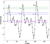 |
Fig. 1 Graphical illustration of the sequence identification procedure that is used to calculate the sample entropy for a simulated light curve. We set r = 0.1 × σligi,t curve and m = 2 in this example. The dashed horizontal lines represent x0 ± r, x\ ± r and x2 ± r. The points that fall within this boundary, namely d[xi,xj] < r, are color-coded in, respectively, purple, blue and green. The first unique sequence or template vector of two components (m = 2) is u1,m = (x0,x1). Two other sequences match this template vector in the light curve, namely the sequences (x30,x31) and (x60,x61). Extending u1 to three components (m + 1) then gives (x0,x1,x2), occurring only once more in the light curve at (x30, x31, x32), as x62 does not fall within the tolerance margin r for the extension of (x60, x61 ) to m + 1. There are thus three matches of length ra for the template vector u1 and two matches for its extension to length m + 1. This procedure is then repeated for all other two component template vectors (ui,m+1 = (x1,x2),…,(xN-2, xN-1)) and their three component extensions (ui,m+1 = (x1,x2,xз),…, (xn-2, xn-1, xn)) |
3 Properties from simulations
We empirically analyze the properties of the MSE for a set of already classified Kepler long-cadence variable star light curves and for simulated light curves. The results form a set of guidelines for the interpretation and use of the MSE.
3.1 Effect of coarse-graining
We start by demonstrating how coarse-graining a light curve affects its properties. The effect of coarse-graining is two-fold: it acts as a (i) low-pass filter and (ii) downsampler for the light curve (Nikulin & Brismar 2004; Valencia et al. 2009). The first effect, the low-pass filter, removes high-frequency variability from the light curve. This is illustrated in Fig. 2, which depicts the light curve, amplitude spectrum and multiscale entropy curve of the γDor pulsator KIC005038228. The top panel shows the effect of the scale factor τ on the variability of the light curve. The light curves are plotted from top to bottom with an increasing τ. It is clear that as τ increases, the short-term variability is filtered out. The bottom left panel illustrates the high-frequency filtering effect on the amplitude spectrum. The dashed lines indicate the Nyquist frequency at each τ. We see that ƒNyquist = 283.2µHz for τ = 1, that is, for the original light curve, but that ƒNyquist decreases toward 28.3 μHz for τ = 10, at which it is no longer possible to detect high frequencies. The bottom right panel shows the MSE curve for this star. The points correspond to the sample entropy value of the light curve in the top plot at a particular τ.
The second effect, downsampling, occurs because coarse-graining is achieved by running a moving average filter with nonoverlapping windows. This downsamples the number of points by a factor τ, and hence also the relative level of variability in the light curve. The downside of this method is that, similar to the Fourier domain, aliasing frequencies might be introduced into the coarse-grained signals (Valencia et al. 2009). Aliasing occurs when the Shannon theorem is violated, that is, if the new sampling rate after coarse-graining is less than twice the highest frequency of the signal. The aliasing frequencies usually artifact themselves as sudden drops in the MSE curve. This is especially the case when the dominant frequency is roughly equal to the Nyquist frequency at a particular τ. We demonstrate this with a simulated signal in Fig. 3. The left column displays the coarse-grained signals of three different sine waves, with initial frequencies (a) ƒ = 11.57μHz, (b) ƒ = 34.72µHz and (c) ƒ = 46.3OµHz. We can see that no aliasing occurs in (a) because  , where Ts is the sampling period. This requirement does not hold anymore for (b) and (c), causing aliasing frequencies to be introduced by the coarse-graining procedure. The dips for (b) and (c) occur at respectively τ = 10 and τ = 6, the point at which ƒNyquist ≈ fsignal The aliasing is not directly a problem for the calculation of the MSE though, because the goal of the MSE is to characterize the regularity and complexity of the time series, and not to directly extract the frequencies causing the variability. The sudden drops in the MSE curve that occur due to coarse-graining actually encode the fact that the signal contains relatively high frequencies on this timescale. They are informative with regard to the frequency content of the signal, and thus to the frequencies of the oscillations.
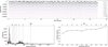 |
Fig. 2 Effect of coarse-graining the γDor star KIC005038228. Top panel: coarse-grained light curves for an increasing τ, which indicates the scaling factor. We use an offset of 20 000 per step (τ) for visualization purposes. Bottom left panel: amplitude spectrum of the original light curve in black. The dashed lines are the Nyquist frequencies at each scaling factor, and illustrate the low-pass filter effect that occurs due to coarse-graining. It is clear from this that the low-pass filter removes the higher frequencies at each step. Bottom right panel: corresponding multiscale entropy curve. Each point on the curve represents the sample entropy calculated for a particular scaling factor. |
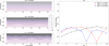 |
Fig. 3 Coarse-grained time series for three different simulated sine waves (left panels; same interpretation as top plot in Fig. 2). The sine waves have an initial frequency of (a) ƒ = 11.57 μHz, (b) ƒ = 34.72 μHz and (c) ƒ = 46.30 μHz. They are interpreted in the same way as the top panel in Fig. 2. The right column (d) shows the MSE curve for each of these different sine waves. |
3.2 Interpretation of MSE curve morphology
Understanding the relation between MSE curve morphology and light curve variability is of prime importance if we want to use the MSE to characterize stellar pulsations. We therefore carefully analyze how the shape of a MSE curve should be interpreted.
The amplitude spectrum in the bottom left panel of Fig. 2 shows the dominant frequencies of the earlier described γ Dor-type star to be in the region around 15 μHz, which is a typical characteristic of g-mode pulsations (3.8 < ƒ < 38.5µHz). There is also a second region with pulsations around 75 μHz, which is typical for p-mode oscillations (34.7 < ƒ < 925.9µHz). The shape of the MSE curve in the bottom right of the figure describes this variability structure by giving an indication of the relative amount of short- and long-term variability that is present in the light curve. When we take a closer look, we see that Se is lower for τ = 1 than for τ = 10, and that the overall slope is positive. This pattern indicates that there is more long- than short-term variability present in the light curve, which coincides with the hybrid pulsation structure found in the amplitude spectrum. The relatively constant Se values between τ = 2 and τ = 5 correspond to the p-modes around 75 μHz.
The positive slope for stars with longer periods occurs because the number of m + 1 sequences (B in Eq. (2)) decreases more rapidly than the number of m sequences (A in Eq. (2)). The number of longer sequences decreases faster because only longer term variability patterns remain after coarse-graining, which, due to their nature, occur much less frequently than short-term patterns, and thus result in less matched patterns overall. We see the opposite effect for stars with only short period variability, as the removal of the short period variability makes the curve more constant and more rapidly increases the number of m + 1 matches given that the whole signal is more similar now.
We confirm this interpretation by comparing the light curves and amplitude spectra for five different types of variability against their MSE curves. The plots are displayed in Fig. 4. Next to the δ Sct and γDor classes, we also examine stars of the aperiodic, constant and solar-like pulsator types. Aperiodic stars have light curves that do not show any clear periodic signal on the examined timescale covered by the light curve (e.g., long-period variables), constant stars have light curves without any statistically significant periodic or aperiodic variability, that is, they only contain white noise, while the light curves of solar-like pulsators are dominated by granulation and stochastically excited high-frequency oscillations (Chaplin & Miglio 2013; García & Ballot 2019). We plot these additional variability types for two reasons. Firstly, they are ideal variability types to benchmark the MSE curves of the δ Sct and γDor stars against. The light curves of constant and aperiodic stars are theoretical opposites of those of pulsators given that they respectively show no significant activity and no periodicity, while the light curves of solar-like stars have granulation and oscillation patterns that are active on similar timescales. Secondly, these additional variability types could potentially also contaminate automatically selected samples of δ Sct and γDor stars. This could, in the case of constant stars, occur because their noise is, similar to the oscillations in δ Sct stars, active on shorter timescales. The light curves of aperiodic stars, on the other hand, might show low-frequency peaks in the Fourier domain, while the red giants in the solar-like pulsator class have lower frequencies that are in the same region as the δ Sct and γDor stars.
The plots in Fig.4 show that the MSE curves of the δ Sct and constant stars both have an opposite slope from that of a γDor star. The downward slope of the δ Sct star and constant star occur because, respectively, their oscillations take place on short timescales and their noise is only present on short timescales, while the positive slope for the γ Dor star occurs because its g-mode oscillations take place on longer timescales. A negative slope thus indicates that a light curve has more short- than long-term variability, while a positive slope indicates that there is more long- than short-term variability present in the light curve. Although the multiscale entropy curves of the δ Sct and constant stars can look similar at first sight, the ensemble analysis with multiple stars in Fig. 5 shows that the MSE curves of constant stars have a much smaller variance and slope compared to those of δ Sct stars. This makes sense given that the light curves of constant stars are pure white noise time series coming from the same Gaussian distribution while the δ Sct light curves come from actual δ Sct stars with pulsations covering a broad frequency region. The sawtooth-like pattern that is seen for some of the δ Sct stars is caused by aliasing frequencies, as discussed in the last paragraph of Sect. 3.1 and illustrated in Fig. 3. The MSE curves of aperiodic stars are monotonically increasing because their light curves only contain information on the longest timescales. The MSE curves of solar-like pulsators follow a pattern similar to those of γDor stars, but have a smaller slope in the beginning and level off near the end. When coupling this to their physical characteristics, we see that this occurs because the granulation is active at lower frequencies while the oscillations take place at higher frequencies, creating two slightly dispersed active regions in the frequency plot. Their variability is thus more, but not perfectly, balanced between the short- and long-term, hence creating a more balanced MSE curve. Figure 5 demonstrates the MSE’s capability to differentiate these five different types of stellar variability.
Audenaert et al. (2021) also snowed the capability of the MSE to distinguish pulsating stars from binary systems and rotational variables. Eclipsing binaries could in most cases also be distinguished from contact binaries and from rotational variables. Contact binaries and rotational variables cannot be distinguished from each other because their light curves are nearly identical in the time domain. Audenaert et al. (2021) therefore grouped these two classes into one overarching class. Theoretically, it should also be possible to distinguish pulsators with signals of rotational modulation from pure pulsators. However, more detailed studies are still required to confirm this, as (i) Audenaert et al. (2021) used the MSE in combination with other attributes and (ii) light curves with instrumental trends ended up in the contact and rotational variables class due to the deliberate absence of a separate class.
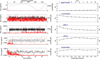 |
Fig. 4 Light curve (left column; black), amplitude spectrum (left column; red), and multiscale entropy curve (right column) for a typical aperiodic, constant, δ Sct, γDor, and solar-like star. |
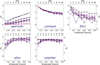 |
Fig. 5 Multiscale entropy curves for ten random stars of the aperiodic, constant, δ Sct, y Dor and solar-like variability type from the training set in Audenaert et al. (2021). |
3.3 Relation with periodicity
The previous sections showed that, in line with Bruce et al. (2009), Mcintosh et al. (2014), Mizuno et al. (2010) and Courtiol et al. (2016), the sample entropy (SE) and multiscale entropy contain information with regard to the frequency content of a signal, or in our case, light curve. We formally test this hypothesis by calculating the Spearman rank correlation matrix between the ten Se that constitute a MSE curve and the first six significant frequencies obtained with the Lomb-Scargle peri-odogram. We calculate the matrix based on the amplitude spectra and MSE curves of the 8328 stars that constitute the training set in Audenaert et al. (2021). The stars in Figs. 4 and 5 also come from this training set. The frequencies that were not significant were replaced with -1 in all tests. The correlation matrix is shown in Fig. 6. We see a clear correlation between the sample entropy values at each τ and the frequencies extracted from the Fourier domain, confirming the relation between the MSE and frequency values.
The second way we test whether the MSE is related to the frequency content of a star, is by training a random forest (Breiman 2001) regressor with the sample entropy values as input and the frequencies as output. This results in a model with R2 ≈ 0.62 when the first three frequencies are predicted as output, and R2 ≈ 0.51 when the first six frequencies are predicted (according to the amplitude’s signal-to-noise ratio), where R2 is the proportion of the variance of the output variables that is explained by the model based on its input variables. A Canonical Correlation Analysis gives similar results. This result was expected from a mathematical point of view, as we showed that a violation of the Shannon theorem results in frequency information being introduced into the MSE curve, and that the slope contains information with regard to the type of variability. Stars with high-frequency oscillations, such as δ Sct stars, only contain information on the smallest timescales. Their initial light curves are therefore characterized by a high amount of complexity, but this complexity decreases with an increasing timescale (τ), as the light curve now starts to approach a flatter signal. Stars with low-frequency oscillations on the other hand, such as γDor stars, only contain information at larger timescales. Their light curves are therefore characterized by a lower amount of initial complexity, but as the scale increases, more of the signal starts to be taken into account and the complexity also increases. Hence, this relation between the frequencies and MSE.
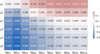 |
Fig. 6 Spearman’s rank-order correlation matrix assessing the correlation between the first six significant frequencies (according to the amplitude’s signal-to-noise ratio) obtained with Lomb-Scargle and the ten sample entropy values that constitute an MSE curve, calculated based on the values of 8328 stars coming from different variability classes. |
3.4 Effect of longer time series
Pincus & Goldberger (1994) already noted that the number of data points affects the calculation of the sample entropy. Costa et al. (2005, Fig. 14) also showed that the confidence intervals of the Se (see Eq. (2)) decrease with the number of data points. The number of data points is an important aspect to be taken into account in high-cadence uninterrupted astronomical data sets, as the number of brightness observations for a star varies per space mission and is often also dependent on its location in the field of view. Depending on the type of oscillations we are interested in, this is of importance to a greater or lesser extent. In order to find stars with low-frequency, low-amplitude g-mode pulsations, for example, we typically need light curves with a longer time base as fewer pulsation cycles are covered in the same period compared to stars with higher-frequency p-modes.
We therefore explore the effect of moving from a time base of 27.4 d, 94 d, 1 yr, 2 yr and 4 yr. These are, respectively, the lengths of single sector TES S data, single Quarter of Kepler data, TESS Continuous Viewing Zone (CVZ) data, PLATO (Rauer et al. 2014) Long Pointing Field (LPF) data and the full length of the Kepler mission. We perform our experiments with long-cadence (30-min) Kepler data, as these light curves go up to lengths of 4 yr and can easily be truncated to shorter time bases.
We find that longer data sets have a positive effect on the robustness of the Se values, but that, starting from a minimum length of ~IOOO data points, the additional increase in robustness is small. The exact effect however, depends on the type of variability (short- vs. long-term). In Fig. 7, we show the MSE curves for the δ Set-type star KIC009655438, for which the light curves have been truncated to the lengths described in the previous paragraph. From a time base of 94d (~45OO data points) on, the shape of the MSE curve becomes very stable and, apart from a slight downward shift, possibly due to the lower uncertainty that originates from the higher number of data points, the curves do not change significantly. In Fig. 8, we show the same plot but for the γ Dor star KIC003343854. We clearly see a larger deviation for the 27 d MSE curve compared to the δ Sct case. This is understandable given that γ Dor stars are low-frequency pulsators; hence, fewer pulsation cycles are covered in the same 27 d period. However, overall, increasing the time base does not drastically improve the MSE curve and good results are already obtained for 27 d light curves, although 94 d might be better for low-frequency variability. This is important given that TESS observes millions of stars at a 27.4 d time base. Lowering the number of data points below ~10m = 1000, does have a much more negative effect on the MSE curve, as stated in Pincus & Goldberger (1994). We conclude that the MSE applied to light curves of only one month is worthwhile for variability classification.
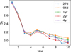 |
Fig. 7 Multiscale entropy curves for the light curve of the δ Sct star KIC009655438 truncated at different lengths. |
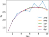 |
Fig. 8 Multiscale entropy curves for the light curve of the y Dor star KIC003343854 truncated at different lengths. |
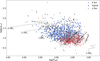 |
Fig. 9 Hertzsprung-Russell diagram showing the log(Teff) and log(L/L⊙) values for our sample of δ Set, γDor and hybrid pulsators originally from Bowman et al. (2016) and Li et al. (2020). The colors and marker style indicate the variability class as listed by Bowman et al. (2016) and Li et al. (2020) based on an inspection of the frequencies in the amplitude spectrum. The hybrid stars of both catalogs have been merged as the catalogs do not indicate whether the hybrid stars are dominantly of the δ Set- or γDor-type. The black solid and dashed lines respectively indicate the δ Sct and γDor theoretical instability strips given by Dupret et al. (2005). The dotted lines are theoretical evolutionary tracks computed by Johnston et al. (2019) for stars between 1.2 M⊙–2.4 M⊙ and solar metallicity. |
4 Discovering hybrids with MSE clustering
We have shown that the MSE is a powerful tool to characterize the light curve structure of a variable star. It is therefore ideally suited as the basis for a clustering framework that can differentiate between different types of pulsators. We specifically focus on separating hybrid pulsators from pure p- and ɡ-mode pulsators in sets of δ Set and γDor stars, as there is no automated tool yet for this that only relies on time domain information, while hybrid stars are prime targets for asteroseismic analysis (Aerts 2021).
We use the catalog with δ Sct stars from Bowman et al. (2016) and the catalog with γDor stars from Li et al. (2020) to demonstrate and validate our methodology. We plot the Hertzsprung-Russell diagram with the log(Teff) and log(L/L⊙) values for all stars in both catalogs in Fig. 9. We used the effective temperature values from the Kepler DR25 input catalog (Mathur et al. 2017) and the luminosities from Murphy et al. (2019). The black solid and dashed lines in the plot respectively show the δ Sct and γDor instability strips from Dupret et al. (2005). The strips only give an indication of the locations of the stars in the diagram however, as they were calculated for specific input physics. Therefore, not all stars in our sample fall within these boundaries. The black dotted lines show the theoretical evolutionary tracks computed by Johnston et al. (2019) for stars between 1.2 M⊙–2.4 M⊙ and solar metallicity, which show that the data are in line with the δ Sct and γDor star mass ranges. We left out ~99 stars from these catalogs for which there were no luminosity values reported in Murphy et al. (2019). We also show a prototypical example of the light curve, amplitude spectrum and MSE curve for a δ Set, δ Set-hybrid, γDor and γDor-hybrid star in Fig. 10.
4.1 Methodology
We first computed the multiscale entropy curve from four-year stitched Kepler light curves with τmax = 10 and m + 1 = 2. We then took the 10 SE values per star that form the MSE2 and used UMAP3 (Uniform Manifold Approximation and Projection for Dimension Reduction; Mclnnes et al. 20l8a,b) to produce a two-dimensional equivalent of the ten-dimensional MSE, in order to avoid working in a high-dimensional data space. UMAP is a dimensionality reduction technique that relies on Riemannian geometry and algebraic topology. The output is similar to the t-SNE dimensionality reduction technique (van der Maaten & Hinton 2008), but UMAP preserves the global structure of the data better and has a lower computational complexity. In order to optimally retain the local density structure of the data, we used densMAP (Narayan et al. 2021), UMAP’s density-preserving equivalent. densMAP uses an estimate of the local density in the original data space as a regularization parameter in the calculation of the two-dimensional UMAP representation. We specifically used the density-preserving version of UMAP because we cluster the data with a density-based algorithm. The two UMAP components are given as input to HDBSCAN4 (Hierarchical Density-Based Spatial Clustering of Applications with Noise; Mclnnes & Healy 2017; Campello et al. 2013), which then provides a cluster structure of the data space that can be analyzed to find subgroups of stars.
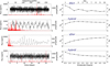 |
Fig. 10 Same as Fig. 4, but for a δ Sct, a γDor and two hybrids. The amplitude spectra and multiscale entropy curves were calculated based on 4 yr of data but we only plot a 27 d excerpt of the light curve for clarity. |
4.2 δ Set star catalog
We take the catalog of 983 δ Set stars compiled by Bowman et al. (2016) and use their original stitched 4yr long-cadence Kepler PDC_SAP light curves. We then apply the steps described in Sect. 4.1 to separate pure δ Set stars with only p-mode pulsations from hybrids with both p- and ɡ-mode pulsations. We set the UMAP parameters to dens_lambda = 5.0, n_neigbours = 25 and min_dist = 0.0, based on UMAP developer advice and our own tests. These parameters respectively control how much of the global and local structure are preserved and how tightly the points are compressed together. For HDBSCAN, we set min_cluster_size = 50 and min_samples = 5, which respectively control the minimum size of a potential cluster and the minimum density that is required for stars to be assigned to a cluster. The results are plotted in Fig. 11, where the colors represent the label of the cluster to which a star belongs.
The plot shows that the data space is separated into two clusters: one cluster of 295 stars and one of 589 stars. We take a random sample of stars from each cluster and perform a visual inspection of their light curves, amplitude spectra and MSE curves. This reveals that cluster 0 mainly consists of hybrid pulsatore with frequencies both in the ɡ-mode and p-mode regime, while cluster 1 mainly consists of δ Set stars with pulsations in the p-mode regime only. Given that HDBSCAN sees clusters as regions in the data space with a high density, not every point gets assigned to a cluster. Points in low-density regions that lie further away from cluster centers are in this sense less certain to belong to a particular cluster and HDBSCAN therefore marks these uncertain points as noise. In this case, we get 99 stars without cluster assignment. A manual extrapolation of the cluster boundaries by means of a line at the intersection of two clusters boundaries would in this case still correctly assign most of these “noisy” stars to one of the two clusters, and therefore also improve the overall classification performance. In Fig. 12, we show the light curve, amplitude spectrum and MSE curve for a representative sample star of each of the clusters from Fig. 11. For the stars that have not been assigned to a cluster, we plot both a star that lies around cluster 1 and a star that lies around cluster 0. One can see that the light curves and amplitude spectra of the stars assigned to cluster 1 are characterized by a high density of p-mode oscillations whereas stars in the “outskirts” of the cluster are characterized by a significantly lower number of the detected p-modes (with the majority of them also showing low amplitudes). Similarly, stars assigned to cluster 0 exhibit rich spectra of both ɡ- and p-modes whereas stars in the outskirts of the cluster show predominantly one type of modes with the other type being significantly underrepresented.
We validate our results by cross-matching the two discovered clusters with the pulsator types assigned by Bowman et al. (2016). The results are displayed in Table 1, where the percentages are expressed in terms of the column totals. We achieve a True Positive Rate of 82.5% for the δ Set stars and 78.1% for the hybrid stars, which confirms that the MSE in combination with UMAP and HDBSCAN can successfully separate hybrid pulsators from pure δ Set stars. The labels from Bowman et al. (2016) were added to Fig. 11 by means of different marker shapes. These labels were not used during the actual clustering procedure. They were only added afterward for the purpose of validation and visualization. We additionally also checked the position in the UMAP plot of two high-amplitude δ Sct stars (HADS; see McNamara 2000 for more details) that were included in the catalog. They appeared to be in the region around the δ Sct cluster, but rather in the low-density noisy part and not in the cluster center. The sample size is however too small to draw any firm conclusions from this.
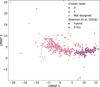 |
Fig. 11 Clustering structure of the δ Set sample from Bowman et al. (2016). The cluster labels are indicated in color and represent the cluster to which the stars are assigned by HDBSCAN based on the density structure of the UMAP components. The “Not assigned” label indicates that the star is seen as noise because it is not close enough to any of the other clusters. The labels from Bowman et al. (2016) are indicated by the marker shapes. Their labels were assigned based on a visual inspection of the light curves and power spectra. These labels were not used during our clustering procedure as it is fully unsupervised. The labels only serve as an indication to better understand the clustering results. The corresponding confusion matrix is shown in Table 1. |
Confusion matrix of the cluster assignments calculated with HDBSCAN and the class labels assigned by Bowman et al. (2016) based on visual inspection.
4.3 γ Dor star catalog
We take the catalog of 611 γDor stars compiled by Li et al. (2020) and use long-cadence Kepler PDC_SAP data to create the light curves. We stitched the individual quarters together by first detrending the light curve of each quarter with a 2nd- (Q1-Q17) or lst-order polynomial (Q0). We remove 6 stars from the catalog as they are known to be part of a binary system, leaving us with 605 light curves. We then apply the same steps as in Sect. 4.2, but instead of differentiating hybrid pulsators from pure δ Sct stars with only p-modes, we now aim to separate hybrid pulsators from pure γDor stars with ɡ-mode pulsations only. We use dens_lambda = 2.0 for UMAP due to a different structure of the clusters. The results are plotted in Fig. 13 and listed in Table 2.
We find again that UMAP is able to successfully reduce the data to two dimensions, but that in this case the clusters are not as dense as in the δ Set star case. The stars with a hybrid pulsation structure are still largely separated from those with ɡ-mode pulsations only, but they are much more spread out in the plot. We find that cluster 0 contains the hybrid pulsators and cluster 1 the pure γDor stars, with respectively 59 and 426 stars in each cluster. We show a prototypical example of a light curve, amplitude spectrum and MSE for each type in, respectively, the fourth and third row of Fig. 10.
One possible cause for the larger dispersion of the data points in Fig. 13 is the effect of rotation. Rotation globally shifts the frequencies of ɡ-modes to higher levels and can therefore potentially push, otherwise similar, light curves away from one another (Van Reeth et al. 2015a; Pápics et al. 2017; Szewczuk et al. 2021). This results in a larger variety of MSE curves and thus in a data space with a lower density, especially if the data set is small. We show the effect of rotation on the MSE in Fig. 14, where, as in Fig. 13, the two UMAP components of the MSE curves are plotted, but this time the stars are color-coded according to their near-core rotation rates frot, as determined by Li et al. (2020). This clearly shows a strong correlation between the elongated and more dispersed shape of the plot and frot, We also take two representative sample stars from each of the two clusters in Fig. 13, one with a high and one with a low value for frot, to illustrate the differences in frequency values and MSE curves that occur due to rotation. The plots are shown in Fig. 15, where one clearly recognizes a shift of ɡ-mode frequencies toward the higher-frequency regime in high frot, stars. Training a random forest regres sor with the MSE values as input and frot, as output, results in R2 ≈ 0.50 ± 0.06, confirming their relation. The variation in R2 depends on the initialization parameters of the random forest and the split of the training and testing set. Fitting the data with a linear regression model gives a similar result, with R2 ≈ 0.57. The structure of the plot might also be affected by the fact that the instrumental trends in the light curves are still relatively large compared to the low-amplitude g-modes of the stars.
The more sparsely sampled data space gives HDBSCAN a more difficult time to cluster hybrid pulsators, resulting in a true positive rate of 59.0% for this class, which is significantly lower than in the δ Set star case. Including the unassigned points by drawing a line at the separation point of the two clusters, increases the true positive rate to around 68.0% for the hybrid class. HDBSCAN has fewer problems with the pure γDor stars here, because they, in contrast, almost all lie on the same line with a relatively high density. This results in a true positive rate of 87.2% for the γDor class.
Same as Table 1 but for the уDor-type and hybrid pulsatore from Li et al. (2020).
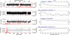 |
Fig. 12 Same as Fig. 4, but for a sample star drawn from each of the clusters in Fig. 11. The amplitude spectra and multiscale entropy curves were calculated based on 4 yr of data but we only plot a 27 d excerpt of the light curve for clarity. |
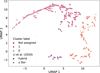 |
Fig. 13 Same as Fig. 11, but for the γDor sample from Li et al. (2020). The corresponding confusion matrix is shown in Table 2. |
5 Conclusions and future prospects
The MSE is a powerful tool to characterize stellar pulsations based on high-cadence uninterrupted photometric light curves. It provides insights into the structure of the variability, relative amount of short- and long-term variability and is related to the frequency content of a star, with the rotational frequency of γDor stars in addition to their pulsations particular. Our analysis reveals that there exists a continuum in which the MSE curves move from δ Sct stars toward hybrid stars toward γDor stars, illustrating its descriptive power for pulsational variability.
We have leveraged this strength of the MSE to characterize stellar pulsation structure for the development of a clustering tool that can differentiate hybrid pulsators with both p- and ɡ-modes from pure pulsators that, respectively, exhibit only p-mode (δ Sct) and ɡ-mode (γDor) pulsations. The framework constitutes an important step toward performing a more in-depth classification of stars observed by the Kepler and TESS missions. It has the potential to serve as a “Level 2” classifier in the T’DA classification framework from Audenaert et al. (2021), in which high-level variability classes such as δ Sct and γDor stars are subdivided into their more detailed constituents, which in our case are stars with only p- or only g-mode pulsations and stars with both p- and ɡ-mode pulsations simultaneously. Hybrid pulsators are important to the asteroseismic community as they allow for more detailed analyses of the internal core and envelope physics. In particular, hybrids allow us to deduce stellar rotation profiles (Aerts et al. 2019, Fig. 4) and gain better insights into the mechanisms that drive stellar pulsations. The MSE in itself is also useful for the study of the rotation as it is strongly correlated to the near-core rotation rates of ɡ-mode pulsators. The MSE might allow us to estimate these near-core rotation rates without having to perform detailed asteroseismic analyses.
The benefit of our MSE-UMAP-HDBSCAN clustering methodology is that, in contrast to supervised classification, it does not require any labeled training samples and the results are highly interpretable given that for the classification we only rely on one feature in the time domain. Operating in the time domain instead of the Fourier domain also does not incur a large loss of information in our case, because the MSE is able to capture the timescales of the stellar variability patterns. The integration of our more detailed unsupervised classifier into the high-level T'DA supervised classifier is in this sense optimal, as the data first gets structured on a high level by the supervised classifier after which the unsupervised classifier can use this information to obtain more detailed insights.
Future work should investigate other clustering setups and test whether the methodology can differentiate between other types of pulsation modes. Instead of first reducing the multiscale entropy curves with UMAP and then clustering the UMAP components with with HDBSCAN, the curves could also be clustered directly with sequential data or time series clustering methods, such as k-Shape (Paparrizos & Gravano 2015) or COBRAS-TS (Van Craenendonck et al. 2018). It should also be investigated whether our clustering tool can actually distinguish the high-amplitude δ Set stars from more typical p-mode δ Sct stars, by means of a larger data sample for the former. Lastly, it would be interesting to see if the methodology is capable of distinguishing mixed modes from p-modes in red giants, pure pulsators from pulsators with rotational modulation and pure pulsators from pulsators in binary systems. The clustering methodology should then be run on the sets of Kepler and TESS δ Sct and γDor stars that will be returned by the T’DA classifier from Audenaert et al. (2021). Our methodology will also be included in the variability classification pipelines of the PLATO mission.
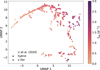 |
Fig. 14 Same as Fig. 13, but color-coded according to the near-core rotation rates from Li et al. (2020). The figure shows that the structure of the UMAP values, and thus the MSE, can partially be explained by frot. |
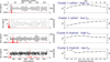 |
Fig. 15 Same as Fig. 4, but for a sample star drawn from each of the clusters in Fig. 13 according to the ƒrot values in Fig. 14. The amplitude spectra and multiscale entropy curves were calculated based on 4 yr of data but we only plot a 27 d excerpt of the light curve for clarity. |
Acknowledgements
The authors respectfully thank the anonymous referee for the thorough yet timely reviews of the manuscript; their enthousiasm is an important encouragement for us. The research leading to these results has received funding from the European Research Council (ERC) under the European Union’s Horizon 2020 research and innovation programme (grant agreement N°670519: MAMSIE), from the KU Leuven Research Council (grant С16/18/005: PARADISE), from the Research Foundation Flanders (FWO) under grant agreement G0H5416N (ERC Runner Up Project), as well as from the BELgian federal Science Policy Office (BELSPO) through PRODEX grant PLATO. J.A. also gratefully acknowledges funding from the Research Foundation Flanders (FWO) by means of a long stay travel grant with grant agreement no. V401922N. The resources and services used in this work were provided by the VSC (Flemish Supercomputer Center), funded by the Research Foundation - Flanders (FWO) and the Flemish Government. This research has made use of NASA’s Astrophysics Data System, as well as the NASA/IPAC Extragalactic Database (NED) which is operated by the Jet Propulsion Laboratory, California Institute of Technology, under contract with the National Aeronautics and Space Administration. This paper includes data collected by the Kepler mission. Funding for the Kepler and K2 mission was provided by NASA’s Science Mission Directorate. TΊie authors acknowledge the efforts of the Kepler Mission team in obtaining the light curve data and data validation products used in this publication. TΊiese data were generated by the Kepler Mssion science pipeline through the efforts of the Kepler Science Operations Center and Science Office. TΊie Kepler light curves are archived at the Mikulski Archive for Space Telescopes. The authors would also like to thank C. Aerts and the MAMSIE/PARADISE team at KU Leuven for their valuable comments and feedback.
References
- Aerts, C. 2021, Rev. Mod. Phys., 93, 015001 [Google Scholar]
- Aerts, C., & Kolenberg, K. 2005, A&A, 431, 615 [NASA ADS] [CrossRef] [EDP Sciences] [Google Scholar]
- Aerts, C., Christensen-Dalsgaard, J., & Kurtz, D. W. 2010, Asteroseismology (Springer, Dordrecht) [Google Scholar]
- Aerts, C., Mathis, S., & Rogers, T. M. 2019, ARA&A, 57, 35 [Google Scholar]
- Armstrong, D. J., Kirk, J., Lam, K. W. F., et al. 2016, MNRAS, 456, 2260 [NASA ADS] [CrossRef] [Google Scholar]
- Audenaert, J., Kuszlewicz, J. S., Handberg, R., et al. 2021, AJ, 162, 209 [NASA ADS] [CrossRef] [Google Scholar]
- Balona, L. A., Guzik, J. A., Uytterhoeven, K., et al. 2011, MNRAS, 415, 3531 [Google Scholar]
- Barbara, N. H., Bedding, T. R., Fulcher, B. D., Murphy, S. J., & Van Reeth, T. 2022, MNRAS, 514, 2793 [NASA ADS] [CrossRef] [Google Scholar]
- Battley, M. P., Armstrong, D. J., & Pollacco, D. 2022, MNRAS, 511, 4285 [NASA ADS] [CrossRef] [Google Scholar]
- Blomme, J., Debosscher, J., De Ridder, J., et al. 2010, ApJ, 713, L204 [NASA ADS] [CrossRef] [Google Scholar]
- Blomme, J., Sarro, L. M., O’Donovan, F.T., et al. 2011, MNRAS, 418, 96 [NASA ADS] [CrossRef] [Google Scholar]
- Borucki, W. J., Koch, D., Basri, G., et al. 2010, Science, 327, 977 [Google Scholar]
- Bowman, D. M., & Kurtz, D. W. 2018, MNRAS, 476, 3169 [NASA ADS] [CrossRef] [Google Scholar]
- Bowman, D. M., Kurtz, D. W., Breger, M., Murphy, S. J., & Holdsworth, D. L. 2016, MNRAS, 460, 1970 [NASA ADS] [CrossRef] [Google Scholar]
- Bradley, P. A., Guzik, J. A., Miles, L. F., et al. 2015, AJ, 149, 68 [CrossRef] [Google Scholar]
- Breiman, L. 2001, Mach. Learn., 45, 5 [Google Scholar]
- Bruce, E. N., Bruce, M. C., & Vennelaganti, S. 2009, J. Clinical Neurophysiol., 26 [Google Scholar]
- Campello, R. J. G. B., Moulavi, D., & Sander, J. 2013, in Advances in Knowledge Discovery and Data Mining, eds. J. Pei, V.S. Tseng, L. Cao, H. Motoda, & G. Xu (Berlin, Heidelberg: Springer Berlin Heidelberg), 160 [Google Scholar]
- Chaplin, W. J., & Miglio, A. 2013, ARA&A, 51, 353 [Google Scholar]
- Costa, M., Goldberger, A. L., & Peng, C. K. 2002, Phys. Rev. Lett., 89, 068102 [NASA ADS] [CrossRef] [Google Scholar]
- Costa, M., Goldberger, A. L., & Peng, C. K. 2005, Phys. Rev. E, 71, 021906 [NASA ADS] [CrossRef] [Google Scholar]
- Courtiol, J., Perdikis, D., Petkoski, S., et al. 2016, J. Neurosci. Methods, 273, 175 [CrossRef] [Google Scholar]
- de Freitas, D. B., Lanza, A. F., da Silva Gomes, F.O., & Das Chagas, M.L. 2021, A&A, 650, A40 [NASA ADS] [CrossRef] [EDP Sciences] [Google Scholar]
- Debosscher, J., Sarro, L. M., Aerts, C., et al. 2007, A&A, 475, 1159 [NASA ADS] [CrossRef] [EDP Sciences] [Google Scholar]
- Debosscher, J., Sarro, L. M., López, M., et al. 2009, A&A, 506, 519 [CrossRef] [EDP Sciences] [Google Scholar]
- Debosscher, J., Blomme, J., Aerts, C., & De Ridder, J. 2011, A&A, 529, A89 [NASA ADS] [CrossRef] [EDP Sciences] [Google Scholar]
- Dupret, M. A., Grigahcène, A., Garrido, R., Gabriel, M., & Scuflaire, R. 2004, A&A, 414, L17 [NASA ADS] [CrossRef] [EDP Sciences] [Google Scholar]
- Dupret, M. A., Grigahcène, A., Garrido, R., Gabriel, M., & Scuflaire, R. 2005, A&A, 435, 927 [NASA ADS] [CrossRef] [EDP Sciences] [Google Scholar]
- Eisner, N. L., Barragán, O., Lintott, C., et al. 2021, MNRAS, 501, 4669 [NASA ADS] [CrossRef] [Google Scholar]
- ESA Special Publication 1997, 1200, The Hipparcos and Tycho Catalogues. Astrometric and Photometric Star Catalogues Derived from the ESA Hipparcos Space Astrometry Mission (Noordwijk, The Netherlands: ESA Publications) [Google Scholar]
- Eyer, L., & Mowlavi, N. 2008, J. Phys. Conf. Ser., 118, 012010 [NASA ADS] [CrossRef] [Google Scholar]
- Gaia Collaboration (Prusti, T., et al.) 2016, A&A, 595, A1 [NASA ADS] [CrossRef] [EDP Sciences] [Google Scholar]
- Gaia Collaboration (De Ridder, J., et al.) 2022, A&A, in press https://doi.org/10.1051/0004-6361/202243767 [Google Scholar]
- García, R. A., & Ballot, J. 2019, Liv. Rev. Sol. Phys., 16, 4 [Google Scholar]
- Gebruers, S., Tkachenko, A., Bowman, D. M., et al. 2022, A&A, 665, A36 [NASA ADS] [CrossRef] [EDP Sciences] [Google Scholar]
- Graham, M. J., Drake, A. J., Djorgovski, S. G., Mahabal, A. A., & Donalek, C. 2013, MNRAS, 434, 2629 [NASA ADS] [CrossRef] [Google Scholar]
- Grigahcène, A., Antoci, V., Balona, L., et al. 2010, ApJ, 713, L192 [Google Scholar]
- Guzik, J. A., Kaye, A. B., Bradley, P. A., Cox, A. N., & Neuforge, C. 2000, ApJ, 542, L57 [Google Scholar]
- Handler, G., & Shobbrook, R. R. 2002, MNRAS, 333, 251 [NASA ADS] [CrossRef] [Google Scholar]
- Hon, M., Stello, D., & Yu, J. 2018a, MNRAS, 476, 3233 [NASA ADS] [CrossRef] [Google Scholar]
- Hon, M., Stello, D., & Zinn, J. C. 2018b, ApJ, 859, 64 [NASA ADS] [CrossRef] [Google Scholar]
- Hon, M., Stello, D., García, R. A., et al. 2019, MNRAS, 485, 5616 [NASA ADS] [Google Scholar]
- Hon, M., Huber, D., Kuszlewicz, J. S., et al. 2021, ApJ, 919, 131 [NASA ADS] [CrossRef] [Google Scholar]
- Johnston, C., Tkachenko, A., Aerts, C., et al. 2019, MNRAS, 482, 1231 [Google Scholar]
- Kurtz, D. W., Saio, H., Takata, M., et al. 2014, MNRAS, 444, 102 [Google Scholar]
- Kuszlewicz, J. S., Hekker, S., & Bell, K. J. 2020, MNRAS, 497, 4843 [NASA ADS] [CrossRef] [Google Scholar]
- Li, G., Van Reeth, T., Bedding, T. R., et al. 2020, MNRAS, 491, 3586 [Google Scholar]
- Lomb, N. R. 1976, Ap&SS, 39, 447 [Google Scholar]
- Mathur, S., Huber, D., Batalha, N. M., et al. 2017, ApJS, 229, 30 [NASA ADS] [CrossRef] [Google Scholar]
- McInnes, L., & Healy, J. 2017, IEEE International Conference on Data Mining Workshops (ICDMW), 33 [CrossRef] [Google Scholar]
- McInnes, L., Healy, J., & Melville, J. 2018a, ArXiv e-prints [arXiv: 1802.03426] [Google Scholar]
- McInnes, L., Healy, J., Saul, N., & Grossberger, L. 2018b, J. Open Source Softw., 3, 861 [CrossRef] [Google Scholar]
- McIntosh, A. R., Vakorin, V., Kovacevic, N., et al. 2014, Cerebral Cortex, 24, 1806 [CrossRef] [Google Scholar]
- McNamara, D. H. 2000, ASP Conf. Ser., 210, 373 [NASA ADS] [Google Scholar]
- Mizuno, T., Takahashi, T., Cho, R. Y., et al. 2010, Clinical Neurophysiol., 121, 1438 [CrossRef] [Google Scholar]
- Modak, S., Chattopadhyay, T., & Chattopadhyay, A. K. 2020, J. Appl. Stat., 47, 376 [CrossRef] [Google Scholar]
- Molnar, C. 2019, Interpretable Machine Learning: A guide for making black box models explainable, ed. Lulu.com, https://christophm.github.io/interpretable-ml-book/ [Google Scholar]
- Mombarg, J. S. G., Van Reeth, T., Pedersen, M. G., et al. 2019, MNRAS, 485, 3248 [NASA ADS] [CrossRef] [Google Scholar]
- Mowlavi, N., Barblan, F., Saesen, S., & Eyer, L. 2013, A&A, 554, A108 [NASA ADS] [CrossRef] [EDP Sciences] [Google Scholar]
- Mowlavi, N., Saesen, S., Semaan, T., et al. 2016, A&A, 595, L1 [NASA ADS] [CrossRef] [EDP Sciences] [Google Scholar]
- Moździerski, D., Pigulski, A., Kopacki, G., Kołaczkowski, Z., & Stęślicki, M. 2014, Acta Astron., 64, 89 [NASA ADS] [Google Scholar]
- Mozsdzierski, D., Pigulski, A., Kołaczkowski, Z., et al. 2019, A&A, 632, A95 [NASA ADS] [CrossRef] [EDP Sciences] [Google Scholar]
- Murphy, S. J., Hey, D., Van Reeth, T., & Bedding, T. R. 2019, MNRAS, 485, 2380 [NASA ADS] [CrossRef] [Google Scholar]
- Narayan, A., Berger, B., & Cho, H. 2021, Nat. Biotechnol., 39, 765 [CrossRef] [Google Scholar]
- Nikulin, V. V., & Brismar, T. 2004, Phys. Rev. Lett., 92, 089803 [NASA ADS] [CrossRef] [Google Scholar]
- Paparrizos, J., & Gravano, L. 2015, in Proceedings of the 2015 ACM SIGMOD International Conference on Management of Data, SIGMOD ’15 (New York, NY, USA: Association for Computing Machinery), 1855 [CrossRef] [Google Scholar]
- Pápics, P.I., Tkachenko, A., Van Reeth, T., et al. 2017, A&A, 598, A74 [NASA ADS] [CrossRef] [EDP Sciences] [Google Scholar]
- Perryman, M. A. C., Lindegren, L., Kovalevsky, J., et al. 1997, A&A, 500, 501 [NASA ADS] [Google Scholar]
- Pincus, S. M. 1991, Proc. Natl. Acad. Sci., 88, 2297 [NASA ADS] [CrossRef] [Google Scholar]
- Pincus, S. M., & Goldberger, A. L. 1994, Am. J. Physiology-Heart Circulatory Physiol., 266, 8184944 [Google Scholar]
- Rauer, H., Catala, C., Aerts, C., et al. 2014, Exp. Astron., 38, 249 [Google Scholar]
- Richman, J. S., & Moorman, J. R. 2000, Am. J. Physiology-Heart Circulatory Physiol., 278, 10843903 [Google Scholar]
- Ricker, G. R., Winn, J. N., Vanderspek, R., et al. 2015, J. Astron. Teles. Instrum. Syst., 1, 014003 [Google Scholar]
- Saesen, S., Carrier, F., Pigulski, A., et al. 2010, A&A, 515, A16 [NASA ADS] [CrossRef] [EDP Sciences] [Google Scholar]
- Saesen, S., Briquet, M., Aerts, C., Miglio, A., & Carrier, F. 2013, AJ, 146, 102 [NASA ADS] [CrossRef] [Google Scholar]
- Sánchez Almeida, J., Trujillo, I., & Plastino, A. R. 2020, A&A, 642, L14 [NASA ADS] [CrossRef] [EDP Sciences] [Google Scholar]
- Sarro, L. M., Debosscher, J., Aerts, C., & López, M. 2009, A&A, 506, 535 [NASA ADS] [CrossRef] [EDP Sciences] [Google Scholar]
- Scargle, J. D. 1982, ApJ, 263, 835 [Google Scholar]
- Shannon, C. E. 1948, Bell Syst. Tech. J., 27, 623 [CrossRef] [Google Scholar]
- Starck, J. L., Murtagh, F., Querre, P., & Bonnarel, F. 2001, A&A, 368, 730 [NASA ADS] [CrossRef] [EDP Sciences] [Google Scholar]
- Szewczuk, W., Walczak, P., & Daszyńska-Daszkiewicz, J. 2021, MNRAS, 503, 5894 [NASA ADS] [CrossRef] [Google Scholar]
- Triana, S. A., Moravveji, E., Pápics, P. I., et al. 2015, ApJ, 810, 16 [Google Scholar]
- Uytterhoeven, K., Moya, A., Grigahcène, A., et al. 2011, A&A, 534, A125 [CrossRef] [EDP Sciences] [Google Scholar]
- Valencia, J. F., Porta, A., Vallverdu, M., et al. 2009, IEEE Trans. Biomedical Eng., 56, 2202 [CrossRef] [Google Scholar]
- Valenzuela, L., & Pichara, K. 2018, MNRAS, 474, 3259 [NASA ADS] [CrossRef] [Google Scholar]
- Van Craenendonck, T., Meert, W., Dumančić, S., & Blockeel, H. 2018, in Lecture Notes in Computer Science, Discovery Science (Cham: Springer International Publishing), 11198, 179 [Google Scholar]
- van der Maaten, L., & Hinton, G. 2008, J. Mach. Learn. Res., 9, 2579 [Google Scholar]
- Van Reeth, T., Tkachenko, A., Aerts, C., et al. 2015a, A&A, 574, A17 [NASA ADS] [CrossRef] [EDP Sciences] [Google Scholar]
- Van Reeth, T., Tkachenko, A., Aerts, C., et al. 2015b, ApJS, 218, 27 [Google Scholar]
The multiscale entropy was originally developed to analyze cardiac interbeat interval time series from ECG recordings.
We used pyEntropy (https://github.com/nikdon/pyEntropy) for the calculations.
All Tables
Confusion matrix of the cluster assignments calculated with HDBSCAN and the class labels assigned by Bowman et al. (2016) based on visual inspection.
Same as Table 1 but for the уDor-type and hybrid pulsatore from Li et al. (2020).
All Figures
|
Fig. 1 Graphical illustration of the sequence identification procedure that is used to calculate the sample entropy for a simulated light curve. We set r = 0.1 × σligi,t curve and m = 2 in this example. The dashed horizontal lines represent x0 ± r, x\ ± r and x2 ± r. The points that fall within this boundary, namely d[xi,xj] < r, are color-coded in, respectively, purple, blue and green. The first unique sequence or template vector of two components (m = 2) is u1,m = (x0,x1). Two other sequences match this template vector in the light curve, namely the sequences (x30,x31) and (x60,x61). Extending u1 to three components (m + 1) then gives (x0,x1,x2), occurring only once more in the light curve at (x30, x31, x32), as x62 does not fall within the tolerance margin r for the extension of (x60, x61 ) to m + 1. There are thus three matches of length ra for the template vector u1 and two matches for its extension to length m + 1. This procedure is then repeated for all other two component template vectors (ui,m+1 = (x1,x2),…,(xN-2, xN-1)) and their three component extensions (ui,m+1 = (x1,x2,xз),…, (xn-2, xn-1, xn)) |
| In the text | |
|
Fig. 2 Effect of coarse-graining the γDor star KIC005038228. Top panel: coarse-grained light curves for an increasing τ, which indicates the scaling factor. We use an offset of 20 000 per step (τ) for visualization purposes. Bottom left panel: amplitude spectrum of the original light curve in black. The dashed lines are the Nyquist frequencies at each scaling factor, and illustrate the low-pass filter effect that occurs due to coarse-graining. It is clear from this that the low-pass filter removes the higher frequencies at each step. Bottom right panel: corresponding multiscale entropy curve. Each point on the curve represents the sample entropy calculated for a particular scaling factor. |
| In the text | |
|
Fig. 3 Coarse-grained time series for three different simulated sine waves (left panels; same interpretation as top plot in Fig. 2). The sine waves have an initial frequency of (a) ƒ = 11.57 μHz, (b) ƒ = 34.72 μHz and (c) ƒ = 46.30 μHz. They are interpreted in the same way as the top panel in Fig. 2. The right column (d) shows the MSE curve for each of these different sine waves. |
| In the text | |
|
Fig. 4 Light curve (left column; black), amplitude spectrum (left column; red), and multiscale entropy curve (right column) for a typical aperiodic, constant, δ Sct, γDor, and solar-like star. |
| In the text | |
|
Fig. 5 Multiscale entropy curves for ten random stars of the aperiodic, constant, δ Sct, y Dor and solar-like variability type from the training set in Audenaert et al. (2021). |
| In the text | |
|
Fig. 6 Spearman’s rank-order correlation matrix assessing the correlation between the first six significant frequencies (according to the amplitude’s signal-to-noise ratio) obtained with Lomb-Scargle and the ten sample entropy values that constitute an MSE curve, calculated based on the values of 8328 stars coming from different variability classes. |
| In the text | |
|
Fig. 7 Multiscale entropy curves for the light curve of the δ Sct star KIC009655438 truncated at different lengths. |
| In the text | |
|
Fig. 8 Multiscale entropy curves for the light curve of the y Dor star KIC003343854 truncated at different lengths. |
| In the text | |
|
Fig. 9 Hertzsprung-Russell diagram showing the log(Teff) and log(L/L⊙) values for our sample of δ Set, γDor and hybrid pulsators originally from Bowman et al. (2016) and Li et al. (2020). The colors and marker style indicate the variability class as listed by Bowman et al. (2016) and Li et al. (2020) based on an inspection of the frequencies in the amplitude spectrum. The hybrid stars of both catalogs have been merged as the catalogs do not indicate whether the hybrid stars are dominantly of the δ Set- or γDor-type. The black solid and dashed lines respectively indicate the δ Sct and γDor theoretical instability strips given by Dupret et al. (2005). The dotted lines are theoretical evolutionary tracks computed by Johnston et al. (2019) for stars between 1.2 M⊙–2.4 M⊙ and solar metallicity. |
| In the text | |
|
Fig. 10 Same as Fig. 4, but for a δ Sct, a γDor and two hybrids. The amplitude spectra and multiscale entropy curves were calculated based on 4 yr of data but we only plot a 27 d excerpt of the light curve for clarity. |
| In the text | |
|
Fig. 11 Clustering structure of the δ Set sample from Bowman et al. (2016). The cluster labels are indicated in color and represent the cluster to which the stars are assigned by HDBSCAN based on the density structure of the UMAP components. The “Not assigned” label indicates that the star is seen as noise because it is not close enough to any of the other clusters. The labels from Bowman et al. (2016) are indicated by the marker shapes. Their labels were assigned based on a visual inspection of the light curves and power spectra. These labels were not used during our clustering procedure as it is fully unsupervised. The labels only serve as an indication to better understand the clustering results. The corresponding confusion matrix is shown in Table 1. |
| In the text | |
|
Fig. 12 Same as Fig. 4, but for a sample star drawn from each of the clusters in Fig. 11. The amplitude spectra and multiscale entropy curves were calculated based on 4 yr of data but we only plot a 27 d excerpt of the light curve for clarity. |
| In the text | |
|
Fig. 13 Same as Fig. 11, but for the γDor sample from Li et al. (2020). The corresponding confusion matrix is shown in Table 2. |
| In the text | |
|
Fig. 14 Same as Fig. 13, but color-coded according to the near-core rotation rates from Li et al. (2020). The figure shows that the structure of the UMAP values, and thus the MSE, can partially be explained by frot. |
| In the text | |
|
Fig. 15 Same as Fig. 4, but for a sample star drawn from each of the clusters in Fig. 13 according to the ƒrot values in Fig. 14. The amplitude spectra and multiscale entropy curves were calculated based on 4 yr of data but we only plot a 27 d excerpt of the light curve for clarity. |
| In the text | |
Current usage metrics show cumulative count of Article Views (full-text article views including HTML views, PDF and ePub downloads, according to the available data) and Abstracts Views on Vision4Press platform.
Data correspond to usage on the plateform after 2015. The current usage metrics is available 48-96 hours after online publication and is updated daily on week days.
Initial download of the metrics may take a while.